
Quantile Regression: Formula, Interpretation Across Quantiles, Python, R, SPSS and Excel
Quantile Regression estimates conditional percentiles of G3 rather than compressing the full conditional distribution into one mean equation. This worked guide fits tau 0.25, 0.50 and 0.75 to 649 complete student records, explains asymmetric check loss, compares coefficient patterns, audits quantile crossing and keeps Python, R, SPSS and Excel evidence separate.
Quantile Regression Model Overview
Quantile Regression models a specified conditional percentile. For the same predictor pattern, tau 0.25 describes a lower conditional grade location, tau 0.50 describes the conditional median and tau 0.75 describes an upper conditional grade location. The three equations are fitted separately, so every coefficient, fitted value, loss and diagnostic must retain its tau label.
The worked model uses G3 as the outcome and G1, G2, studytime, failures, absences, age, school, sex and address as predictors. All 649 complete rows contribute to every fit. The lower model is not restricted to low-scoring students, and the upper model is not restricted to high-scoring students.
The central estimating principle is asymmetric absolute loss. A residual above the fitted surface and a residual below the surface receive different weights unless tau equals 0.50. At the median, Quantile Regression minimizes absolute deviation and estimates a conditional median rather than the conditional mean estimated by Ordinary Least Squares Regression.
Research Question
The analysis asks whether prior grades and student characteristics relate differently to lower, central and upper conditional locations of final grade. That question is more detailed than a single mean model because a predictor can have a different slope at the lower quartile than at the median or upper quartile.
When to Use Quantile Regression
Use Quantile Regression when a percentile is the scientific target, when spread changes across covariate patterns, when lower or upper conditional performance matters, or when one mean equation is an incomplete description. The method is particularly informative when the outcome distribution is asymmetric or contains boundary concentrations.
When Not to Use It Automatically
The method does not eliminate the need to specify functional form, factor coding, dependence or a defensible validation plan. Extreme quantiles require more information than central quartiles, and independent equations can cross. A model selected only because normality is inconvenient may still be poorly specified.
Comparison with Related Methods
Ordinary Least Squares Regression estimates a conditional mean using squared loss. Robust Regression can protect a mean estimator from unusually large residuals while retaining a mean target. The Interquartile Range summarizes unconditional spread, whereas fitted q25 and q75 are covariate-specific conditional locations.
Verified Numerical Pattern
Python pinball losses are 194.500023, 244.875001 and 175.750023 at tau 0.25, 0.50 and 0.75. The matching pseudo R-squared values are 0.686417, 0.685453 and 0.715500. These numbers measure relative improvement in tau-specific loss, not variance explained.
The lower and upper Python solutions assign G2 a slope close to 1 while many other slopes are close to zero. The median equation distributes information across G1, G2, failures and age. Because G3 is discrete and G1 and G2 are correlated, different optimizers can reach close loss values with different coefficient vectors.
Quick Answer
What Quantile Regression estimates
- Tau 0.25 estimates the lower conditional quartile.
- Tau 0.50 estimates the conditional median.
- Tau 0.75 estimates the upper conditional quartile.
- All observations enter all three objectives.
What the saved evidence shows
- G2 is the dominant positive predictor across tau.
- The median G2 coefficient is 0.794872.
- The median failures coefficient is −0.205128.
- Python and R have close losses but different coefficients.
Table of Contents
- Why this analysis needs Quantile Regression
- How Quantile Regression works
- Variables and data dictionary
- Complete Quantile Regression results
- Eight Python chart stories
- Four R charts and explanations
- Coefficient interpretation
- Predictions, losses and crossing evidence
- Assumptions and diagnostics
- Python, R, SPSS and Excel workflows
- Code
- Advanced Quantile Regression topics
- APA-style reporting
- Publication checklist
- Downloads
- Related Salar Cafe guides
- Frequently asked questions
Why This Analysis Needs Quantile Regression
A conditional mean can be accurate on average while failing to describe lower and upper outcome locations. Students with identical recorded predictors can still have a wide, asymmetric or bounded conditional grade distribution. Quantile Regression allows the fitted relationship to change across that distribution.
The source outcome is bounded and integer-valued. Ties and grade concentrations make the conditional distribution especially relevant because one mean and one residual standard deviation can conceal important location-specific behavior. Percentiles and Quartiles provides the descriptive foundation, while this model adds covariate conditioning.
Changing variance is another reason to examine several conditional locations. A White Test can assess heteroscedasticity in an OLS comparison, but it does not estimate the lower, median and upper conditional surfaces directly.
How Quantile Regression Works
Conditional Quantile Equation
Every coefficient carries a tau label. Holding the remaining design columns fixed, a one-unit predictor increase changes the fitted conditional tau quantile by the corresponding coefficient.
Check-Loss Objective
When a prediction is below the observation, the residual is positive and receives weight tau. When a prediction is above the observation, the absolute residual receives weight 1 − tau. The asymmetry moves the fitted surface toward the requested conditional percentile.
Four-Step Workflow
Keep G3 on its original scale and use the same numeric predictors and factor references at every tau.
Estimate tau 0.25, 0.50 and 0.75 separately, then recalculate fitted loss, null loss and pseudo R-squared.
Check calibration, coefficient stability, software differences and q25 ≤ q50 ≤ q75 before interpretation.
Pseudo R-Squared
For the Python median equation, 1 − 244.875001 / 778.5 = 0.685453. The quantity compares two median-loss objectives. It is not an ordinary squared-deviation ratio.
Why Optimizers Can Differ
The objective is convex but nonsmooth at zero residuals. Tied grades and correlated columns can create flat optimal regions. Python and R can therefore produce similar predictions and objective values while distributing coefficients differently.
Variables Used, Coding and Standardization
The same 649 complete observations and nine-column design are used at every tau. Numeric variables remain on their original scales. School, sex and address use treatment coding so their coefficients are adjusted category contrasts.
| Role | Variable | Saved coding | Quantile Regression interpretation |
|---|---|---|---|
| Outcome | G3 | Observed final grade | Conditional grade percentile on the original scale |
| Prior grade | G1 | Numeric grade points | Change in the fitted tau quantile per G1 point |
| Prior grade | G2 | Numeric grade points | Change in the fitted tau quantile per G2 point |
| Study behavior | studytime | Ordered study-time code | Linear fitted shift per coded level at the selected tau |
| Academic history | failures | Previous failure count or code | Conditional quantile shift per failure unit |
| Attendance | absences | Absence count | Conditional quantile shift per absence |
| Demographic | age | Years | Conditional quantile shift per year |
| Factor | school | GP reference; MS indicator | MS-minus-GP contrast at the selected tau |
| Factor | sex | Female reference; male indicator | Male-minus-female contrast at the selected tau |
| Factor | address | Rural reference; urban indicator | Urban-minus-rural contrast at the selected tau |
Treating studytime as categorical, recoding a reference group or adding nonlinear terms creates a different model. All tau equations must be refitted whenever the design matrix changes.
Complete Quantile Regression Results
Tau 0.25 loss improvement
Tau 0.50 loss improvement
Tau 0.75 loss improvement
Null loss 620.25
Null loss 778.5
Independent-fit ordering audit
Python Objective and Fit Summary
| Target | Tau | n | Fitted pinball loss | Null loss | Pseudo R² | Iterations |
|---|---|---|---|---|---|---|
| Lower conditional quartile | 0.25 | 649 | 194.500023 | 620.25 | 0.686417 | 48 |
| Conditional median | 0.50 | 649 | 244.875001 | 778.5 | 0.685453 | 506 |
| Upper conditional quartile | 0.75 | 649 | 175.750023 | 617.75 | 0.715500 | 40 |
| OLS conditional-mean benchmark | Mean | 649 | Different objective | Different objective | OLS R² = 0.852222 | Not applicable |
Interpretation of the Objective Values
The upper conditional quartile has the largest relative reduction in its matching intercept-only loss. The median model uses the greatest number of saved optimizer iterations, but iteration count is not a measure of model quality.
The three pseudo R-squared values are loss-improvement ratios. They do not state that 68.6%, 68.5% or 71.6% of G3 variance is explained. For the ordinary variance-based definition, use the internal R Squared guide.
Python and R Cross-Check
Python and R reach close objective values but do not return identical coefficient vectors. The Python median loss is 244.875001, while the independently saved R median loss is 245.068163 with pseudo R² 0.685205. Those results remain software-specific because tied integer outcomes and correlated prior grades create flat regions in the piecewise-linear objective.
Open the Verified Output Files
The source reports support the results, coefficient estimates and chart explanations.
Eight Python Chart Stories
The eight Python figures follow the attached post pattern: visible pattern, exact values, interpretation and why the evidence matters.
Python Chart 1: G3 Distribution and Quantile Context
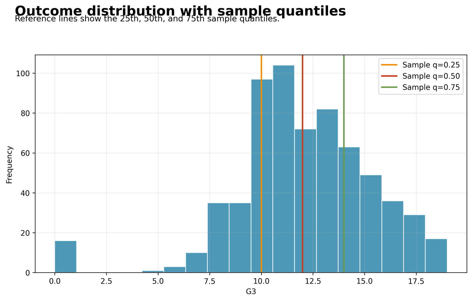
The same-topic outcome distribution used for all three conditional quantile fits.
Quantile regression tau=0.25
The same-topic outcome distribution used for all three conditional quantile fits. Discrete grade concentrations and boundaries create ties in the check-loss problem. Those ties help explain why different optimizers can find nearby losses with different coefficient allocations.
The plot establishes the observed range before any conditional percentile is interpreted.
Python Chart 2: Lower-Quartile Calibration
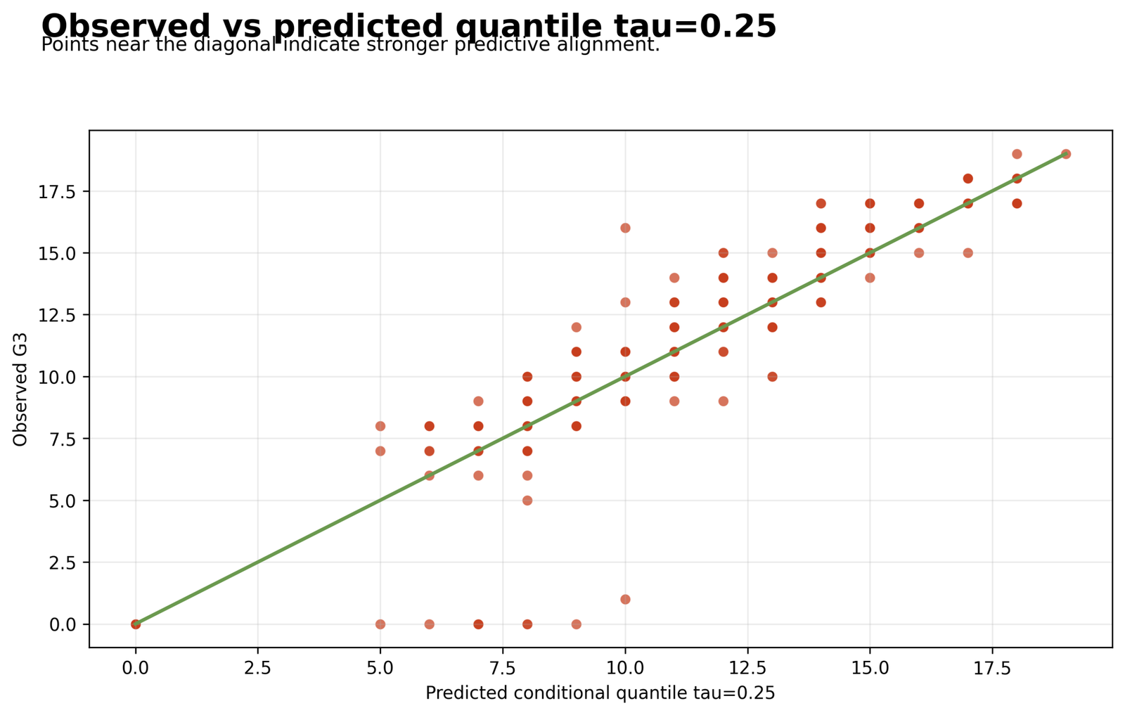
Observed G3 against the fitted tau 0.25 conditional quantile.
Observed G3 against the fitted tau 0.25 conditional quantile.
Observed G3 against the fitted tau 0.25 conditional quantile. This panel asks whether the lower conditional boundary tracks the observed covariate pattern. It is not expected to behave like an OLS prediction scatter centered symmetrically on an identity line.
Count the direction of residuals and inspect predictor regions where the lower fit systematically misses.
Python Chart 3: Median Calibration
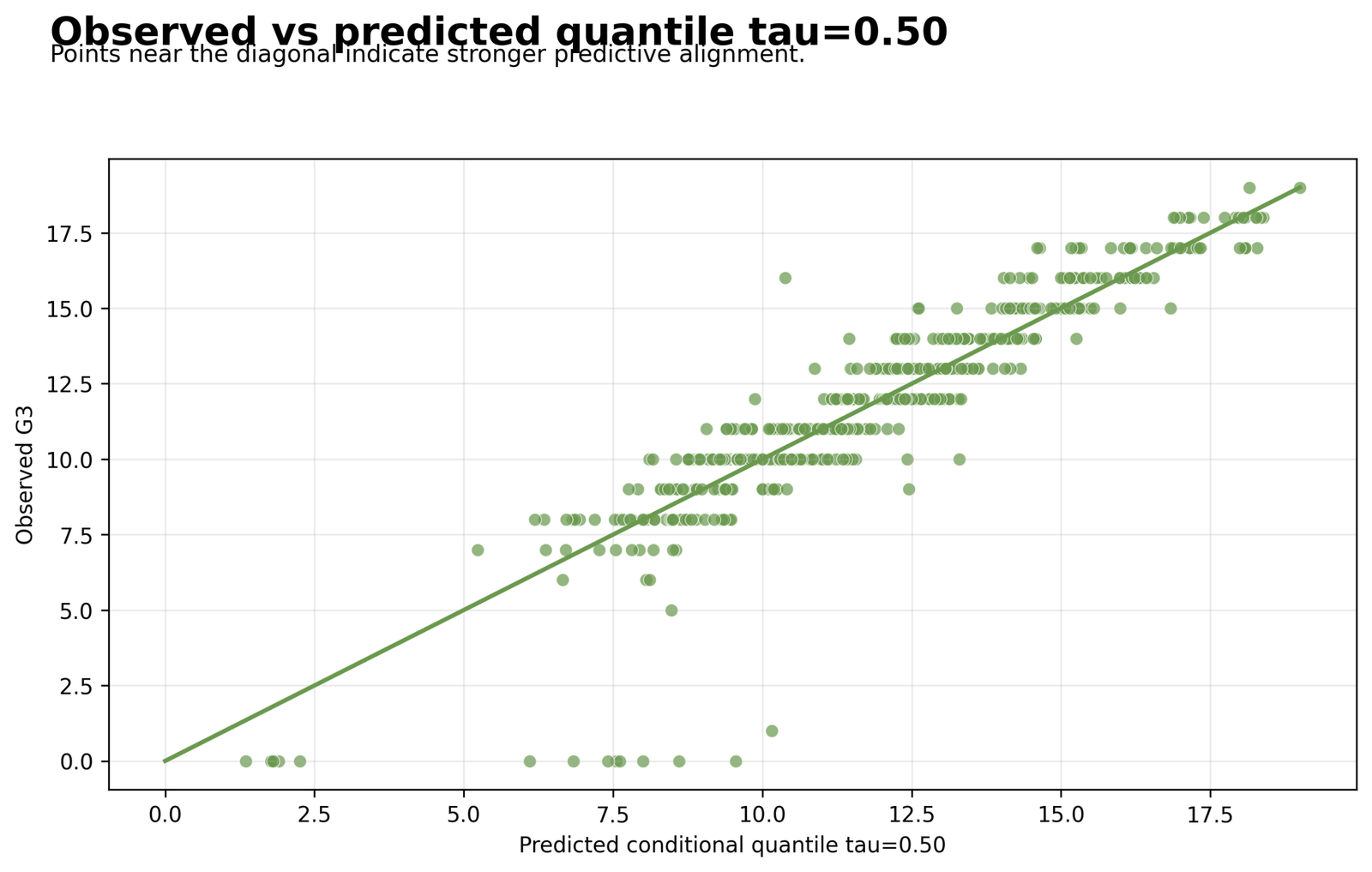
Observed G3 compared with the tau 0.50 median-regression prediction.
Observed G3 compared with the tau 0.50 median-regression prediction.
Observed G3 compared with the tau 0.50 median-regression prediction. The fitted value divides conditional mass rather than minimizing squared error. Persistent imbalance above and below the median curve would challenge calibration.
The saved pseudo R-squared 0.685453 belongs to this median loss comparison.
Python Chart 4: Upper-Quartile Calibration
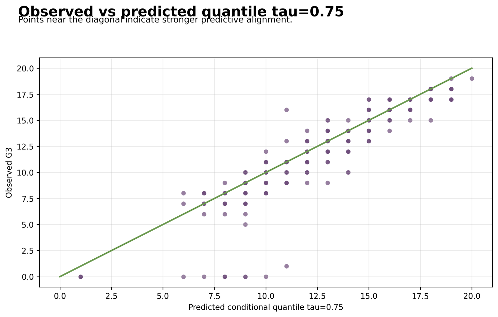
Observed scores against the fitted 75th conditional percentile.
Observed scores against the fitted 75th conditional percentile.
Observed scores against the fitted 75th conditional percentile. The upper equation should leave a larger share of observations below its fitted value than the median equation. Boundaries near the top of G3 can compress its behavior.
Read the panel with the 0.75 pinball loss rather than with OLS residual expectations.
Python Chart 5: Median Residual Structure
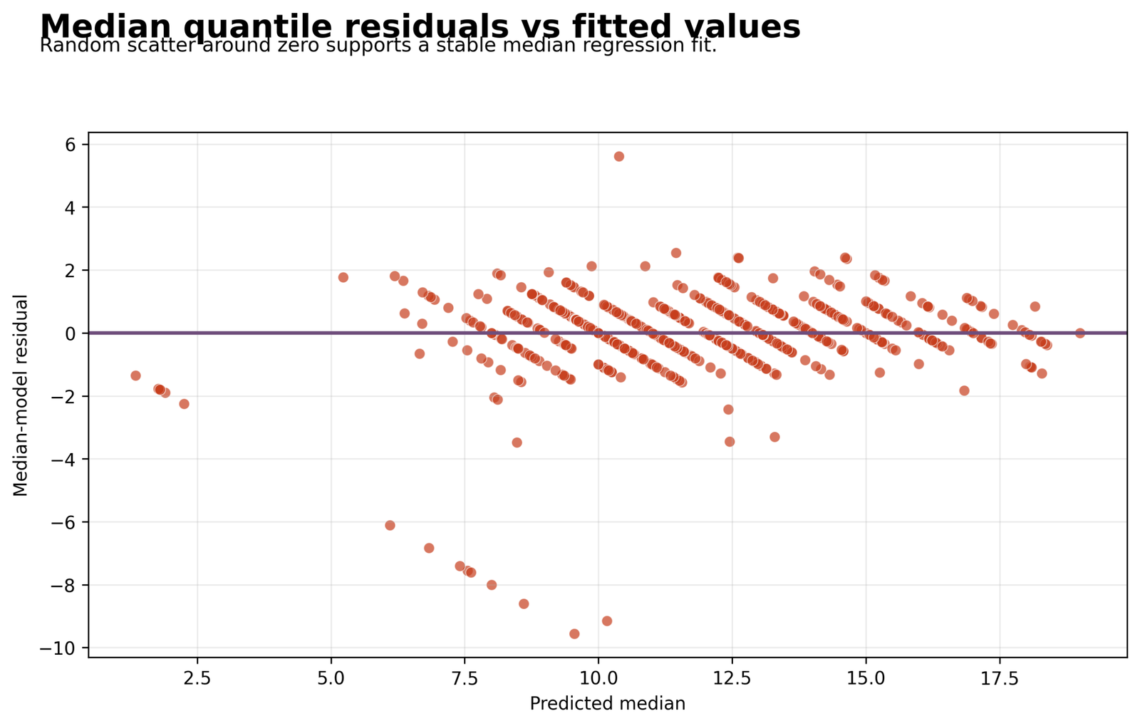
Tau 0.50 residuals plotted over fitted conditional medians.
Tau 0.50 residuals plotted over fitted conditional medians.
Tau 0.50 residuals plotted over fitted conditional medians. Absolute-loss estimation tolerates nonnormal residuals, but a curved center or changing sign balance can still expose a weak linear specification.
Large points should be traced in the prediction ledger before any robustness claim is made.
Python Chart 6: Residual Distributions Across Tau
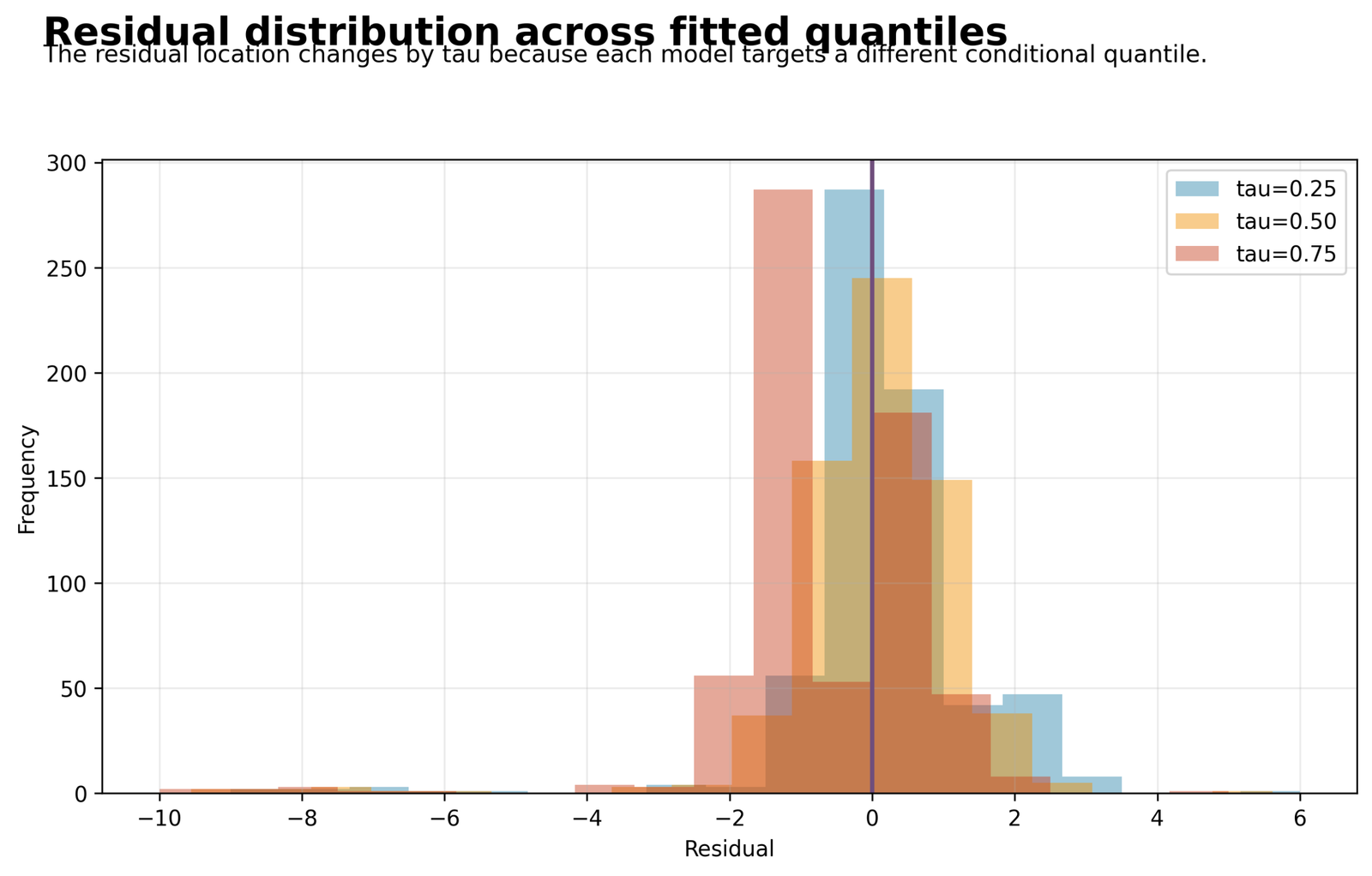
Side-by-side residual behavior for 0.25, 0.50, and 0.75 fits.
Side-by-side residual behavior for 0.25, 0.50, and 0.75 fits.
Side-by-side residual behavior for 0.25, 0.50, and 0.75 fits. Each distribution is shifted by its target percentile and therefore should not be centered using one common rule. Differences show how the fitted location moves through the conditional outcome.
The comparison is most useful for asymmetry and tail behavior, not a normality test.
Python Chart 7: Coefficient Heterogeneity
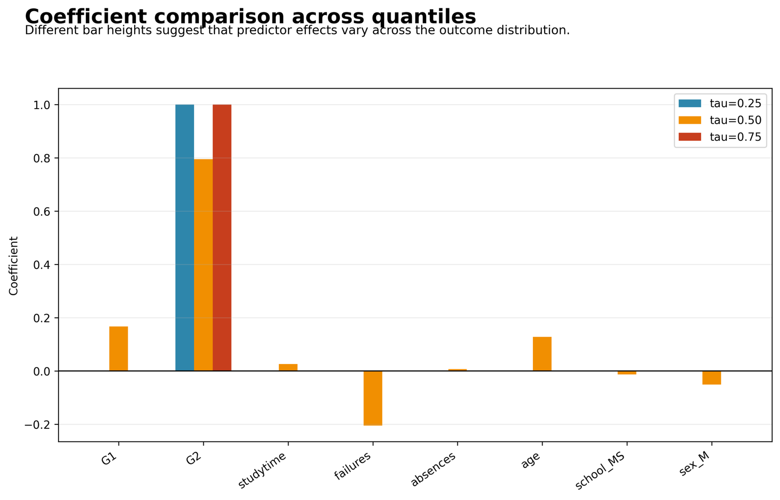
Saved slope estimates compared across the three quantile levels.
Do not call the 0.50 coefficient an average effect; it shifts the conditional median.
Saved slope estimates compared across the three quantile levels. Movement across tau is the direct visual test of whether one mean coefficient hides distributional variation. G1 and G2 should be interpreted with their correlation and confidence intervals in mind.
A dramatic point-estimate swing that lacks interval separation may reflect numerical instability rather than a reliable difference.
Python Chart 8: Pinball Loss by Target
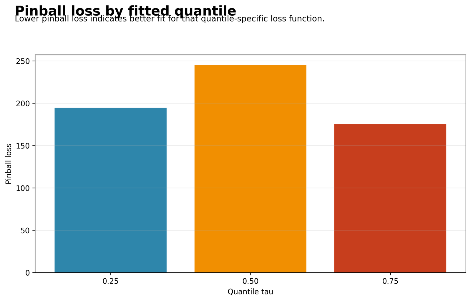
Optimized asymmetric loss for tau 0.25, 0.50, and 0.75.
Optimized asymmetric loss for tau 0.25, 0.50, and 0.75.
Optimized asymmetric loss for tau 0.25, 0.50, and 0.75. The loss values use different asymmetric weights, so their heights require matching null denominators. Pseudo R-squared supplies that within-tau normalization.
Optimizer status and iteration count provide context but do not replace fit interpretation.
R Charts and Paired Explanations
The four verified R images are arranged in two responsive pairs. R provides an independent Quantile Regression cross-check, not a source of replacement decimals for the Python estimates.
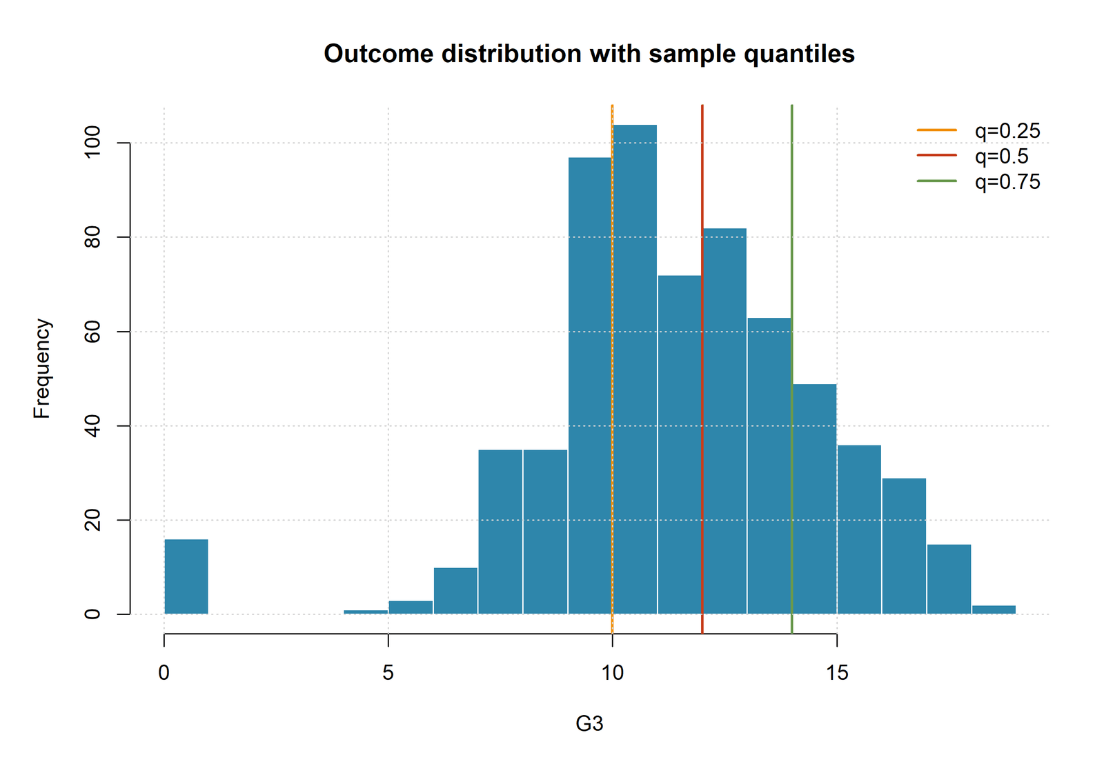
R Chart 1: Outcome and Tie Structure
The integer grade concentrations confirm the nonsmooth, tied-response setting shared by both software workflows.
Exact context: n = 649, with tau 0.25, 0.50 and 0.75 estimated separately.
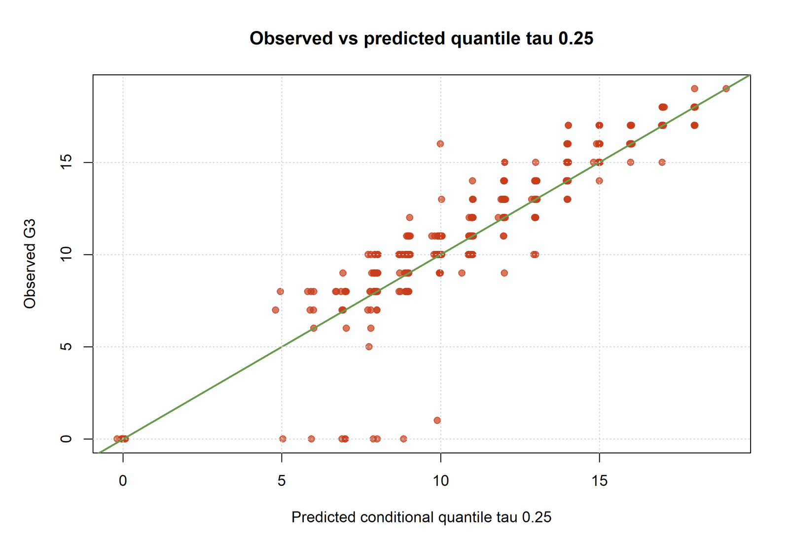
R Chart 2: Lower-Quartile Prediction
The R q25 surface follows the same broad lower-location pattern but arises from a separate coefficient solution.
Exact comparison: Python q25 loss = 194.500023; R q25 loss = 195.446717.
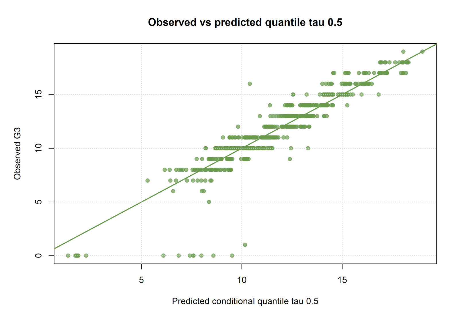
R Chart 3: Median Prediction
The R median surface targets the conditional center under absolute loss and should be read separately from the OLS mean prediction.
Exact comparison: R loss = 245.068163 and pseudo R² = 0.685205; Python loss = 244.875001 and pseudo R² = 0.685453.
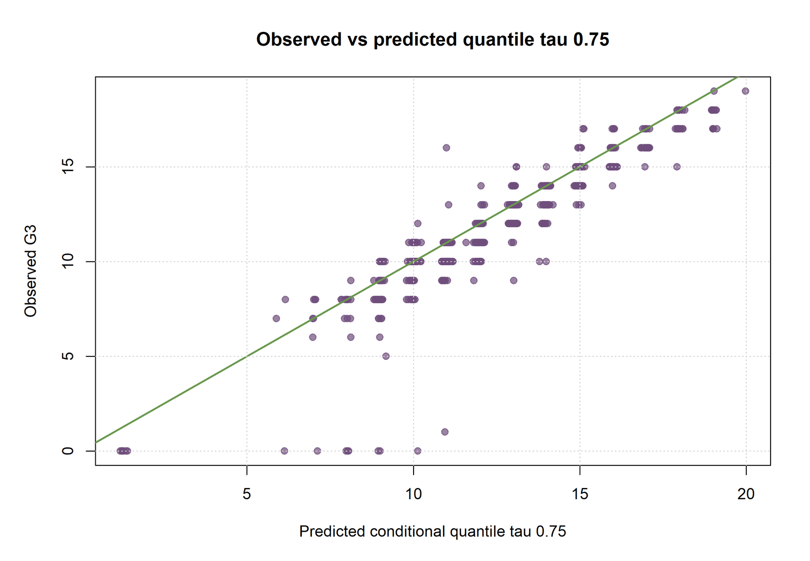
R Chart 4: Upper-Quartile Prediction
The upper R surface describes a higher conditional location and provides a visual check against the Python q75 pattern.
Exact context: Python q75 pseudo R² = 0.715500, the largest relative improvement among the three Python fits.
Quantile Regression Coefficient Interpretation
| Tau | Term | B | SE | p | 95% CI | Interpretation |
|---|---|---|---|---|---|---|
| 0.25 | Intercept | −0.0000014 | 0.337934 | .999997 | −0.663596 to 0.663594 | Reference-profile lower conditional quartile |
| 0.25 | G1 | 0.0000002 | 0.015437 | .999987 | −0.030313 to 0.030314 | Near-zero slope in the saved Python q25 optimum |
| 0.25 | G2 | 1.000000 | 0.015524 | <.001 | 0.969516 to 1.030483 | Dominant lower-quantile grade-progression slope |
| 0.50 | Intercept | −1.384611 | 0.659040 | .036036 | −2.678757 to −0.090465 | Conditional-median anchor for the zero/reference profile |
| 0.50 | G1 | 0.166667 | 0.031153 | <.001 | 0.105491 to 0.227842 | Positive shift in the fitted conditional median |
| 0.50 | G2 | 0.794872 | 0.028934 | <.001 | 0.738054 to 0.851690 | Largest positive median slope |
| 0.50 | failures | −0.205128 | 0.080268 | .010833 | −0.362750 to −0.047506 | Lower fitted median per failure unit |
| 0.50 | age | 0.128205 | 0.036887 | .000544 | 0.055770 to 0.200640 | Positive conditional-median association |
| 0.75 | Intercept | 0.999998 | 0.390359 | .010643 | 0.233457 to 1.766538 | Reference-profile upper conditional quartile |
| 0.75 | G1 | 0.0000003 | 0.016509 | .999985 | −0.032419 to 0.032419 | Near-zero slope in the saved Python q75 optimum |
| 0.75 | G2 | 1.000000 | 0.014012 | <.001 | 0.972485 to 1.027515 | Dominant upper-quantile grade-progression slope |
| 0.75 | failures | −0.0000002 | 0.052582 | .999998 | −0.103255 to 0.103255 | Near-zero saved q75 slope |
Median Coefficients
At tau 0.50, a one-point increase in G2 is associated with a 0.794872-point increase in the fitted conditional median of G3, holding the remaining design columns fixed. This is a median association, not an average effect.
G1 is also positive at the median, while failures is negative. Age is positive in the saved Python median solution. The correct inferential context is tau-specific and software-specific; use Regression P Value and Confidence Interval only as general reporting guides.
Lower and Upper Conditional Quartiles
The q25 and q75 Python solutions allocate nearly all prior-grade progression to G2. That result is compatible with a flat optimum under tied grades and correlated G1/G2 columns. It should not be converted into a claim that G1 has no relationship at every conditional location.
Factor References and Intercepts
GP school, female sex and rural address are the saved reference categories. Intercepts correspond to zero numeric predictors and those references, which is not a realistic student profile. Centering could improve the anchor but would require refitting all three equations.
Predictions, Pinball Loss and Crossing Contributions
Tau-Specific Prediction
Every predictor profile receives three independently estimated conditional locations. The complete evidence file retains observed G3, all three fitted values, the three row-level pinball losses and the OLS mean benchmark for all 649 observations.
How Individual Rows Build the Objective
For a positive residual, the loss is tau multiplied by the residual. For a negative residual, the loss is 1 − tau multiplied by the absolute residual. Summing the row contributions reproduces the fitted objectives in the results table.
| Case | Observed G3 | Fitted q25 | Fitted q50 | Fitted q75 | Median loss | Ordering audit |
|---|---|---|---|---|---|---|
| 1 | 11 | 10.999998 | 9.820514 | 11.999997 | 0.589743 | q25 > q50 |
| 2 | 11 | 11.000000 | 11.179487 | 11.999999 | 0.089744 | Ordered |
| 5 | 13 | 13.000000 | 12.961539 | 13.999999 | 0.019230 | q25 > q50 |
| 9 | 17 | 16.000000 | 15.833333 | 16.999999 | 0.583333 | q25 > q50 |
| 13 | 12 | 13.000000 | 12.923076 | 13.999999 | 0.461538 | q25 > q50 |
| 19 | 7 | 7.999996 | 7.935897 | 9.000000 | 0.467948 | q25 > q50 |
Quantile Crossing
The full audit identifies 65 rows where q25 is above q50 and 15 rows where q50 is above q75. These 80 records demonstrate that the three independently fitted equations do not form an automatically ordered prediction band.
Crossing values must remain visible. Silently sorting q25, q50 and q75 would change the estimated model after fitting and conceal the coherence problem. For general residual concepts, see Residual Analysis.
Prediction Meaning
A fitted quantile is a conditional distribution location for a covariate profile. It is not the probability that one student will attain or exceed that score, and q25 to q75 is not automatically a calibrated prediction interval.
Quantile Regression Assumptions and Diagnostics
Verified model evidence
- 649 complete observations at every tau
- q25 pseudo R² = 0.686417
- q50 pseudo R² = 0.685453
- q75 pseudo R² = 0.715500
- Python and R objectives remain close
Diagnostic cautions
- 80 rows contain fitted quantile crossing
- Tied integer grades create flat objective regions
- G1 and G2 are strongly correlated prior grades
- Standard errors depend on the saved solution
- Training loss is not future validation
Functional Form
The linear predictor must adequately describe each requested conditional quantile. Curvature can differ across tau, so a satisfactory median equation does not prove that the lower and upper surfaces are also linear. Compare with the internal Generalized Additive Model guide when nonlinear structure is scientifically plausible.
Calibration
Inspect the proportions below, equal to and above each fitted surface. Tied G3 scores create equality groups, so continuous-response calibration rules should not be applied mechanically.
Quantile Ordering
Check q25 ≤ q50 ≤ q75 for every predictor pattern. The 80 verified crossing rows are a coherence diagnostic and should be reported, not silently corrected.
Residual and Influence Review
Signed residuals determine the asymmetric loss. High-leverage predictor patterns can still alter Quantile Regression even though residuals are not squared. Review Influence Diagnostics alongside the tau-specific residual plots.
Sampling Structure
Observations and covariance calculations must reflect independence, clustering or repeated measures in the source design. The present saved analysis treats the 649 records as independent complete cases.
Software Stability
Compare objective values, fitted predictions and coefficient patterns across implementations. Close loss with different coefficients is evidence of numerical sensitivity, not permission to average the solutions.
Out-of-Sample Validation
Refit coding, transformations and all tau equations inside each training sample. Evaluate pinball loss and calibration separately at tau 0.25, 0.50 and 0.75 on observations not used for estimation.
Quantile Regression in Python, R, SPSS and Excel
Python
- Fit each tau with statsmodels QuantReg.
- Export coefficients, fitted values and convergence details.
- Recalculate pinball and null losses independently.
- Flag q25/q50 and q50/q75 crossing by row.
R
- Use identical rows, formula and factor references.
- Record the quantreg method and covariance procedure.
- Keep R coefficients with R objective values.
- Compare fitted patterns before individual decimals.
SPSS
- Confirm that the installed procedure estimates conditional quantiles.
- Specify 0.25, 0.50 and 0.75 explicitly.
- Verify category references and confidence intervals.
- Do not substitute ordinary linear regression output.
Excel
- Audit predictions and residual signs.
- Recalculate row and total pinball loss.
- Recalculate null loss and pseudo R-squared.
- Use Solver only with a documented tau-specific objective.
Code and Formula Panels
Python statsmodels Quantile Regression workflow
import numpy as np
import pandas as pd
import statsmodels.formula.api as smf

df = pd.read_csv("dataset.csv")
formula = (
    "G3 ~ G1 + G2 + studytime + failures + absences + age "
    "+ C(school) + C(sex) + C(address)"
)

def pinball_loss(actual, predicted, tau):
    residual = actual - predicted
    return np.where(
        residual >= 0,
        tau * residual,
        (1 - tau) * (-residual)
    )

rows = []
predictions = pd.DataFrame({"row": np.arange(1, len(df) + 1), "observed": df["G3"]})

for tau in (0.25, 0.50, 0.75):
    fit = smf.quantreg(formula, data=df).fit(q=tau, max_iter=10000)
    fitted = fit.predict(df)
    loss = pinball_loss(df["G3"].to_numpy(), fitted.to_numpy(), tau)

    null_quantile = df["G3"].quantile(tau, interpolation="linear")
    null_pred = np.repeat(null_quantile, len(df))
    null_loss = pinball_loss(df["G3"].to_numpy(), null_pred, tau).sum()

    predictions[f"q{int(tau * 100)}"] = fitted
    predictions[f"loss_q{int(tau * 100)}"] = loss

    rows.append({
        "tau": tau,
        "n": int(fit.nobs),
        "pinball_loss": float(loss.sum()),
        "null_loss": float(null_loss),
        "pseudo_r_squared": 1 - float(loss.sum()) / float(null_loss),
        "iterations": fit.iterations,
    })

    fit.summary2().tables[1].to_csv(
        f"quantile_coefficients_tau_{tau:.2f}.csv"
    )

pd.DataFrame(rows).to_csv("quantile_fit_summary.csv", index=False)
predictions.to_csv("quantile_predictions.csv", index=False)
R quantreg workflow
library(quantreg)

dat <- read.csv("dataset.csv")
dat$school <- factor(dat$school)
dat$sex <- factor(dat$sex)
dat$address <- factor(dat$address)

form <- G3 ~ G1 + G2 + studytime + failures + absences + age +
  school + sex + address

taus <- c(0.25, 0.50, 0.75)
fits <- lapply(taus, function(tau) {
  rq(form, tau = tau, data = dat, method = "br")
})

pinball <- function(actual, predicted, tau) {
  u <- actual - predicted
  ifelse(u >= 0, tau * u, (1 - tau) * (-u))
}

summary_rows <- lapply(seq_along(taus), function(i) {
  tau <- taus[i]
  fit <- fits[[i]]
  pred <- as.numeric(predict(fit, newdata = dat))
  fitted_loss <- sum(pinball(dat$G3, pred, tau))
  null_value <- as.numeric(quantile(dat$G3, probs = tau, type = 7))
  null_loss <- sum(pinball(dat$G3, rep(null_value, nrow(dat)), tau))

  data.frame(
    tau = tau,
    n = nrow(dat),
    pinball_loss = fitted_loss,
    null_loss = null_loss,
    pseudo_r_squared = 1 - fitted_loss / null_loss
  )
})

write.csv(do.call(rbind, summary_rows),
          "quantile_r_fit_summary.csv", row.names = FALSE)

for (i in seq_along(taus)) {
  write.csv(
    as.data.frame(summary(fits[[i]], se = "nid")$coefficients),
    sprintf("quantile_r_coefficients_tau_%.2f.csv", taus[i])
  )
}
SPSS quantile-command outline
* Quantile Regression command availability depends on SPSS version.
* Confirm the installed procedure and preserve the tau label.

* Example outline when QUANTILE REGRESSION is available.
QUANTILE REGRESSION G3 WITH
 G1 G2 studytime failures absences age
 BY school sex address
 /QUANTILE=0.25 0.50 0.75
 /PRINT=PARAMETER COVB
 /CRITERIA=CILEVEL(95).

* Export fitted quantiles and calculate pinball loss separately.
* Do not substitute ordinary linear regression coefficients
* for a requested conditional quantile model.
Excel pinball-loss and crossing formulas
Excel quantile-regression audit

1. Residual for one tau
=ObservedCell-PredictedQuantileCell

2. Pinball loss
=IF(ResidualCell>=0,
    TauCell*ResidualCell,
    (1-TauCell)*ABS(ResidualCell))

3. Total fitted loss
=SUM(PinballLossRange)

4. Null fitted quantile
=PERCENTILE.INC(ObservedRange,TauCell)

5. Null loss
Apply the same pinball formula using the null quantile
as the predicted value for every row.

6. Pseudo R-squared
=1-(FittedLossCell/NullLossCell)

7. Crossing flag
=IF(OR(Q25Cell>Q50Cell,Q50Cell>Q75Cell),
    "Crossing","Ordered")

Excel can audit predictions and losses. Estimating all coefficients
requires Solver or imported software results and must preserve the
factor coding and tau-specific objective.
Advanced Quantile Regression Topics
1. The Conditional Quantile Target
Quantile Regression estimates a percentile of the outcome distribution after conditioning on the predictor pattern. The target at tau 0.25 is therefore the lower conditional quartile for each covariate profile, not the quartile calculated once from all 649 observed grades.
Report the tau label beside every equation and compare this conditional target with the unconditional definitions in Percentiles and Quartiles. Omitting tau removes the identity of the parameter.
2. Why Every Row Enters Every Fit
All 649 observations contribute to each objective. The lower model is not estimated from the lowest 25 percent of students, and the upper model is not estimated from the highest 25 percent.
The asymmetric weights determine the fitted location. Subgroup restriction would answer a different, selection-biased question and would not reproduce the supplied coefficients or pinball losses.
3. Check Loss and Residual Direction
The check-loss function assigns different weights to positive and negative residuals. At tau 0.25, an overprediction receives weight 0.75 and an underprediction receives weight 0.25. The pattern reverses at tau 0.75.
At tau 0.50 the two weights are equal, so Quantile Regression minimizes one-half of the total absolute error. The scaling constant does not change the coefficient minimizer.
4. Loss-Based Pseudo R-Squared
The reported pseudo R-squared is one minus fitted pinball loss divided by intercept-only pinball loss at the same tau. It measures improvement in the selected asymmetric loss.
It is not the variance decomposition used by Ordinary Least Squares Regression. The values 0.686417, 0.685453 and 0.715500 must not be described as percentages of variance explained.
5. Discrete Grade Outcomes
G3 is bounded and integer-valued. Tied outcomes create many residuals that can be exactly zero at a candidate solution and can produce flat portions of the piecewise-linear objective.
This geometry helps explain the extremely simple Python lower- and upper-quartile coefficient vectors. It also makes optimizer sensitivity and crossing diagnostics more important than they would be with a smooth continuous response.
6. Nonunique Coefficient Solutions
A convex objective can have more than one minimizing coefficient vector when the design and tied outcomes create a flat optimum. Numerical convergence therefore does not guarantee a unique scientific allocation among correlated predictors.
Keep each coefficient vector attached to its own software, objective value, inference method and fitted predictions. Do not average Python and R estimates to manufacture a solution that neither program fitted.
7. Correlated Prior Grades
G1 and G2 contain strongly overlapping grade-progression information. At the lower and upper Python optima, G2 receives a slope near one while G1 is near zero; the median fit distributes information across both.
This redistribution is conditional and model-dependent. Review the same design from a mean-model perspective in Multiple Linear Regression without treating one model as a significance test for the other.
8. Quantile Crossing
Independent fitting does not enforce q25 less than or equal to q50 less than or equal to q75. The supplied prediction ledger has 65 q25-above-q50 rows and 15 q50-above-q75 rows, for 80 observations with at least one ordering violation.
Crossing does not erase the fitted objectives, but it prevents the three equations from being advertised as an automatically coherent interval. Constrained estimation or post-estimation rearrangement would be a new analysis.
9. Calibration with Ties
A fitted conditional tau quantile should place the outcome below and above the surface in proportions compatible with tau, subject to sampling variation and ties. Integer outcomes can produce a large equality group.
Report counts below, equal to and above the fitted value rather than forcing a continuous-response calibration rule. Equality is substantive information in this grade dataset.
10. Standard Errors and Confidence Intervals
Quantile standard errors depend on how the conditional density or sparsity near the target quantile is estimated. Tied outcomes can make asymptotic estimates sensitive to bandwidth and covariance choices.
The interval must remain attached to the corresponding coefficient solution. General interpretation of significance can be reviewed in Regression P Value, but OLS standard errors must never be copied onto Quantile Regression slopes.
11. Python Optimization Record
The Python fits report 48, 506 and 40 iterations at tau 0.25, 0.50 and 0.75. Iteration count describes the numerical path, not predictive quality or scientific importance.
Preserve the software version, tolerance, maximum iterations and convergence message. A successful status should be accompanied by an independent recomputation of fitted pinball loss.
12. R Optimization Record
The R workflow is an independent cross-check with its own optimization route and standard-error implementation. Its median loss of 245.068163 is close to the Python value 244.875001 but not identical.
Close objectives support similar overall fit, while coefficient differences disclose numerical or identification sensitivity. The R result should not be relabeled as a replication of every Python decimal.
13. Comparing Objective Values Correctly
Raw pinball losses at different tau values use different residual weights and different intercept-only benchmarks. The smallest raw loss does not identify the best quantile model.
Compare fitted and null loss within the same tau, then interpret pseudo R-squared and calibration. Cross-tau model choice is primarily a scientific-target decision, not a competition for one minimum number.
14. The OLS Benchmark
OLS remains useful because it estimates the conditional mean from the same predictors. The supplied OLS R-squared of 0.852222 and the quantile pseudo R-squared values use different objectives and denominators.
Use Ordinary Least Squares Regression to understand the mean equation. Do not rank it against a quantile fit by comparing the two R-squared labels directly.
15. Robust Mean versus Conditional Median
Median Quantile Regression estimates the conditional 50th percentile. Robust mean procedures may reduce the impact of large residuals while continuing to estimate a conditional mean.
The estimands remain different even when both appear less sensitive to outliers than OLS. See Robust Regression for the mean-focused alternative.
16. Nonlinear Conditional Quantiles
The current equations are linear in the supplied design columns. Curvature in G1, G2, age or absences would require polynomial terms, splines or another nonlinear quantile specification.
A Generalized Additive Model illustrates flexible conditional-mean modeling. Flexible quantiles require their own validated basis functions and cannot be inferred from the current linear fits.
17. Heteroscedasticity and Distribution Shape
Changing spread is one reason to examine multiple conditional locations. Different slopes across tau can describe distributional changes that one mean equation and one residual-variance summary cannot show.
A White Test evaluates heteroscedasticity in an OLS comparison, whereas Quantile Regression directly estimates selected conditional locations.
18. Dependence and Clustered Samples
The supplied analysis treats rows as independent. When observations are clustered by classroom, school, family or repeated measurement, the coefficient target and uncertainty calculation must reflect that dependence.
Cluster-robust covariance or multilevel quantile methods may be needed. A large row count does not compensate for an incorrectly specified sampling unit.
19. Influence and Unusual Cases
Quantile Regression does not square residuals, but high-leverage design points can still alter a fitted conditional surface substantially. Influence can vary with tau.
Review Influence Diagnostics and compare fitted equations after justified sensitivity checks. Do not delete observations solely because they change a coefficient.
20. Missing Data
The worked analysis uses 649 complete rows. Complete-case estimation is transparent, but its validity depends on why other records are missing and whether the retained sample represents the intended population.
Any imputation model must be fitted without leaking validation outcomes and should preserve the bounded, discrete grade structure. Quantile Regression is not itself a missing-data method.
21. Factor Coding
School, sex and address are treatment-coded. Their coefficients compare one category with the declared reference while every numeric predictor is held fixed.
Changing a reference category changes the intercept and displayed contrasts but not fitted values when the same column space is preserved. Every report should state GP, female and rural as the references used here.
22. Quartile Curves Are Not Prediction Intervals
The distance between fitted q25 and q75 describes an estimated conditional interquartile span. It is not automatically a 50 percent prediction interval with guaranteed coverage.
Crossing, estimation uncertainty and model misspecification affect coverage. The descriptive Interquartile Range guide provides context but does not replace validation of conditional curves.
23. Out-of-Sample Validation
The supplied metrics are in-sample optimization summaries. Deployment claims require a protected validation design that fits the complete preprocessing and coefficient estimation process on training data.
Evaluate tau-specific pinball loss, calibration, crossing and subgroup behavior on unseen observations. New-data validation is more informative than reporting additional training-set decimals.
24. Extreme Quantiles
Tau 0.25, 0.50 and 0.75 have reasonable central support. More extreme levels such as 0.05 or 0.95 rely on fewer effective observations and can produce substantially greater uncertainty.
Extreme-tail analyses require larger samples, stronger diagnostics and often specialized methods. The current central-quartile evidence should not be extrapolated automatically.
25. Software-Specific Reporting
A complete result names the software, estimator, optimization method, tau, standard-error method and factor coding. These details are part of the statistical result, not optional technical notes.
Python and R outputs should be presented side by side when they differ. SPSS and Excel should be described according to what was actually estimated or audited rather than assumed capability.
26. Quantile Regression Decision Framework
Choose Quantile Regression because the research question concerns a conditional percentile or changing distributional location. Prespecify tau, coding, functional form and inference method before comparing results.
Fit each model, verify the objective, inspect crossing and calibration, compare with Regression Diagnostics, and reserve substantive conclusions for patterns supported across estimates, uncertainty and validation.
APA-Style Reporting
Separate Quantile Regression models estimated the conditional 25th, 50th and 75th percentiles of G3 from G1, G2, studytime, failures, absences, age, school, sex and address among 649 students. Python pseudo R-squared values were .686, .685 and .716, calculated from fitted and intercept-only pinball loss at the corresponding tau values.
At tau = .50, G2 was positively associated with the conditional median of G3, b = 0.795, 95% CI [0.738, 0.852], and G1 was also positive, b = 0.167, 95% CI [0.105, 0.228]. Failures was negative, b = −0.205, 95% CI [−0.363, −0.048], whereas several remaining intervals included zero.
The Python q25 and q75 solutions placed G2 near 1.000 and most other slopes near zero. Independent R optimization produced similar objective values but different coefficient allocations. The case-level ledger contained 80 observations with at least one fitted-order violation, so the three equations were not interpreted as an automatically coherent prediction interval.
Publication Checklist
Include
- G3 as the outcome and n = 649
- Tau 0.25, 0.50 and 0.75
- Numeric predictors and factor references
- Check-loss definition
- Fitted and matching null loss
- Loss-based pseudo R-squared definition
- Tau-specific coefficients and intervals
- Software, optimizer and inference method
- Python and R results kept separate
- All 80 crossing rows disclosed
Avoid
- Calling pseudo R-squared variance explained
- Calling tau 0.25 a lowest-quarter subgroup model
- Calling a median coefficient an average effect
- Comparing raw losses across tau without null loss
- Averaging Python and R coefficients
- Sorting crossing predictions after estimation
- Calling q25 to q75 a guaranteed interval
- Transferring OLS p-values to quantile slopes
- Ignoring ties and correlated predictors
- Using training loss as deployment accuracy
Downloads and Verification Resources
Frequently Asked Questions
What is Quantile Regression?
It estimates a selected conditional percentile of an outcome. The slope vector can differ at tau 0.25, 0.50 and 0.75.
What does tau represent?
Tau is the target conditional percentile level. Tau 0.25 is the lower conditional quartile, tau 0.50 is the conditional median and tau 0.75 is the upper conditional quartile.
Does tau 0.25 use only the lowest 25 percent of students?
No. Every observation contributes to the tau 0.25 objective. Residual direction determines the asymmetric weight.
What is pinball loss?
Pinball or check loss is an asymmetric absolute-error function. Its positive and negative residual weights are determined by tau.
Is pseudo R-squared the percentage of variance explained?
No. It is the relative reduction in pinball loss compared with an intercept-only quantile model at the same tau.
What are the verified Python pseudo R-squared values?
They are 0.686417 at tau 0.25, 0.685453 at tau 0.50 and 0.715500 at tau 0.75.
How should the median G2 coefficient be interpreted?
The value 0.794872 means that a one-point G2 increase shifts the fitted conditional median of G3 upward by about 0.794872 points, holding the other design columns fixed.
Why are the q25 and q75 Python equations so simple?
Tied integer grades, correlated prior-grade predictors and a flat nonsmooth objective can support solutions with G2 near one and many other slopes near zero.
Why do Python and R coefficients differ?
They use different numerical procedures and inference implementations. Close objective values can coexist with different coefficient allocations.
How many fitted quantile crossings were found?
The case ledger contains 80 observations with at least one ordering violation: 65 have q25 above q50 and 15 have q50 above q75.
Does median regression require normal residuals?
No normal residual distribution is required for the conditional median estimator, but independence, functional form and valid uncertainty estimation still matter.
Can raw pinball losses be compared across tau?
Not by themselves. Each tau uses different weights and a different null benchmark, so fitted loss must be paired with the matching null loss.
Are q25 and q75 a prediction interval?
They are estimated conditional quartile curves. Crossing and estimation uncertainty prevent automatic guaranteed-coverage interpretation.
Why retain an OLS comparison?
OLS provides a conditional-mean benchmark and clarifies how mean and percentile targets differ. Its R-squared is not directly comparable with quantile pseudo R-squared.
What should be checked on new data?
Evaluate tau-specific pinball loss, calibration, crossing, coefficient stability and relevant subgroup behavior on a protected validation sample.
Which internal guides support this analysis?
Read Percentiles and Quartiles, Ordinary Least Squares Regression, Robust Regression and Regression Diagnostics.
Quantile Regression Conclusion
Quantile Regression estimates three conditional locations of G3 from the same 649-row design. The Python pseudo R-squared values are 0.686417 at tau 0.25, 0.685453 at tau 0.50 and 0.715500 at tau 0.75. The upper conditional quartile has the largest relative improvement in its own pinball-loss benchmark.
G2 is the dominant positive predictor at every tau. The median equation also assigns visible slopes to G1, failures and age. The simpler lower and upper Python coefficient vectors must be interpreted alongside tied integer outcomes, correlated grade predictors and the independent R optimization.
The case-level evidence identifies 80 observations with at least one fitted-order violation. Consequently, q25, q50 and q75 are reported as independent conditional surfaces rather than an automatically ordered prediction interval.
The strongest report keeps tau, objective, software, coefficient uncertainty, fitted values, crossing and validation limitations connected. Every contextual link in this rewrite points to a relevant page on onlineinternetcafe.com.
Quantile Regression evidence should remain attached to its tau-specific objective, software implementation and validation record.
Quantile Regression must retain its tau-specific objective, coefficient vector, software implementation, crossing diagnostic and validation target. Quantile Regression pseudo R-squared remains a loss ratio. Quantile Regression coefficients remain conditional percentile associations. Quantile Regression predictions require ordering and calibration checks. Quantile Regression findings must not be converted into causal effects.
Quantile Regression reports every coefficient with tau. Quantile Regression compares each fitted loss with its matching null loss. Quantile Regression keeps Python and R solutions separate. Quantile Regression discloses crossing before prediction use. Quantile Regression requires tau-specific validation on new observations.

