R Squared: Formula, Interpretation, Python, R, SPSS and Excel Guide
R Squared summarizes how much observed outcome sum-of-squares variation is represented by a fitted regression equation. This worked guide audits the exact 649-record G3 model through SST, SSR, SSE, adjusted fit, nested changes, single-predictor comparisons, coefficient context, residual diagnostics and software calculations.
R Squared Model Overview
R Squared, also called the coefficient of determination, compares the squared errors from a fitted regression with the total squared deviations from the observed outcome mean. The worked equation predicts final grade G3 from G1, G2, studytime, failures, absences, age, school and sex.
The model uses 649 complete records. Six predictors are numeric and two are represented by binary indicator parameters, giving eight predictor degrees of freedom and 640 residual degrees of freedom after the intercept is estimated.
The total sum of squares is 6763.2665639445295. The fitted residual sum of squares is 1000.6264252027902. Their difference is regression sum of squares 5762.640138741739. These quantities reconcile exactly, so the reported R Squared can be verified without trusting a software label.
The result means that the exact eight-predictor fitted equation accounts for approximately 85.205% of observed in-sample G3 sum-of-squares variation. It does not mean 85.205% of students are predicted correctly, and it does not assign that percentage causally to the predictors.
Adjusted R Squared is 0.8502004547744846. It charges ordinary fit for estimating eight predictor parameters. The modest reduction indicates that the complexity penalty is small relative to the fitted improvement over the intercept-only model.
Multiple R is 0.9230654537333927. The fitted RMSE using N is 1.2416912922846717 grade points, MAE is 0.7802749614309105 and residual standard error using 640 residual degrees of freedom is approximately 1.250391454457107.
Quick Answer
What R Squared establishes
- The complete fitted model reduces squared error by 85.205% relative to the observed-mean baseline.
- Adjusted fit remains close at 85.020%.
- The global F statistic is 460.722603 with p far below .001.
- G2 creates the largest declared nested increase.
What R Squared does not establish
- It is not an individual prediction-accuracy percentage.
- It does not prove correct functional form or normal residuals.
- It does not divide explained variation uniquely among correlated predictors.
- It is not external validation because these are fitted-sample values.
Table of Contents
- Model Overview
- Quick Answer
- Why R Squared Is Needed
- How R Squared Works
- Variables and Coding
- Verified Results
- Python Chart Stories
- R Chart Pairs
- Coefficient Interpretation
- Predictions and Meaning
- Assumptions and Diagnostics
- Python, R, SPSS and Excel
- Code and Formulas
- Advanced Topics
- APA-Style Reporting
- Publication Checklist
- Downloads
- Related Guides
- Frequently Asked Questions
- Conclusion
Why This Analysis Needs R Squared
The research question asks how much observed G3 dispersion is represented by one eight-predictor linear equation. R Squared is appropriate because the model uses ordinary least squares with an intercept and a continuous outcome, so the fitted residual ledger has a clear observed-mean benchmark.
The statistic is needed alongside, not instead of, prediction errors and diagnostics. RMSE and MAE retain grade-point units. Residual plots reveal whether the unexplained fraction is concentrated in a small number of difficult observations. Adjusted fit and validation address complexity and generalization.
How R Squared Works
Total, Explained and Residual Variation
SST measures observed G3 dispersion around the observed mean before predictors are used. In this analysis SST = 6763.2665639445295.
SSE measures fitted error around the model predictions. The 649 residual squares sum to 1000.6264252027902.
For this OLS model with an intercept, explained and residual variation sum to total variation.
Adjusted Formula
Substituting n = 649, p = 8 and ordinary fit = 0.8520498318760341 gives 0.8502004547744846.
Four-Step Verification Workflow
The global F statistic compares the complete model with an intercept-only model. Here F(8, 640) = 460.72260284941916 with p = 9.428883902712601 × 10−260. This establishes strong collective fitted signal but does not measure its practical prediction error.
Variables Used, Coding and Standardization
| Variable | Role | Coding or unit | Interpretation in the model |
|---|---|---|---|
| G3 | Outcome | Final grade points | Continuous response whose observed sum-of-squares variation is summarized. |
| G1 | Numeric predictor | First-period grade point | First term in the nested sequence. |
| G2 | Numeric predictor | Second-period grade point | Dominant single-predictor fit and largest nested increment. |
| studytime | Numeric predictor | Ordered study-time code | Entered as a one-unit linear score. |
| failures | Numeric predictor | Prior failure count | Entered linearly with a negative fitted coefficient. |
| absences | Numeric predictor | Absence count | Entered linearly in the complete equation. |
| age | Numeric predictor | Years | Entered linearly after absences. |
| school | Categorical predictor | MS versus GP reference | One indicator parameter in the eight-parameter model. |
| sex | Categorical predictor | Male versus female reference | Final indicator in the declared nested order. |
No predictor standardization is required to calculate R Squared; rescaling a predictor without changing the represented linear information does not change fitted values. Coding and reference groups remain important for coefficient interpretation.
Verified R Squared Results
Model and Variance Ledger
| Metric | Exact value | Interpretation |
|---|---|---|
| Complete observations | 649 | Identical rows feed every fitted table and chart. |
| Predictor df / residual df | 8 / 640 | Six numeric terms plus two indicator parameters. |
| SST | 6763.2665639445295 | Total observed G3 sum of squares. |
| SSR | 5762.640138741739 | Regression sum of squares. |
| SSE | 1000.6264252027902 | Residual sum of squared fitted errors. |
| R Squared | 0.8520498318760341 | 85.205% fitted sum-of-squares reduction. |
| Adjusted R Squared | 0.8502004547744846 | Fit after the complexity adjustment. |
| Multiple R | 0.9230654537333927 | Positive square root of fitted R Squared. |
| F statistic | 460.72260284941916 | Global test with 8 and 640 degrees of freedom. |
| Fitted RMSE / MAE | 1.2416912922846717 / 0.7802749614309105 | Outcome-unit fitted error metrics. |
Nested Model Changes
| Step | Added term | R Squared | Adjusted R Squared | Change | F change | p-value |
|---|---|---|---|---|---|---|
| 1 | G1 | 0.6829156800171083 | 0.6824255960604114 | 0.6829156800171083 | 1393.466713 | < .001 |
| 2 | G2 | 0.8477615336889918 | 0.8472902071679050 | 0.1648458536718834 | 699.497466 | < .001 |
| 3 | studytime | 0.8482905263275349 | 0.8475849008685932 | 0.0005289926385431 | 2.249037 | 0.134187 |
| 4 | failures | 0.8494743269157664 | 0.8485393848469203 | 0.0011838005882315 | 5.064701 | 0.024755 |
| 5 | absences | 0.8505634419896496 | 0.8494014158775940 | 0.0010891150738832 | 4.686276 | 0.030772 |
| 6 | age | 0.8506322461601578 | 0.8492362858438975 | 0.0000688041705081 | 0.295728 | 0.586762 |
| 7 | school | 0.8511574154720293 | 0.8495319894319422 | 0.0005251693118715 | 2.261675 | 0.133103 |
| 8 | sex | 0.8520498318760341 | 0.8502004547744846 | 0.0008924164040048 | 3.860398 | 0.049871 |
Coefficient Context
| Term | B | SE | t | p-value | 95% CI |
|---|---|---|---|---|---|
| Intercept | −0.181255 | 0.774670 | −0.233977 | 0.815077 | [−1.702456, 1.339946] |
| school: MS versus GP | −0.197911 | 0.112293 | −1.762452 | 0.078470 | [−0.418419, 0.022596] |
| sex: male versus female | −0.203144 | 0.103392 | −1.964789 | 0.049871 | [−0.406173, −0.000115] |
| G1 | 0.133173 | 0.036760 | 3.622791 | 0.000315 | [0.060989, 0.205358] |
| G2 | 0.880212 | 0.034132 | 25.788245 | 4.198 × 10−101 | [0.813188, 0.947237] |
| studytime | 0.062030 | 0.063222 | 0.981143 | 0.326893 | [−0.062118, 0.186177] |
| failures | −0.227071 | 0.094719 | −2.397303 | 0.016802 | [−0.413068, −0.041073] |
| absences | 0.017974 | 0.011153 | 1.611575 | 0.107547 | [−0.003927, 0.039876] |
| age | 0.024013 | 0.043527 | 0.551694 | 0.581350 | [−0.061459, 0.109486] |
The coefficient table does not allocate the complete R Squared. G2 has a large conditional slope and dominant stand-alone fit, but correlated predictors share variation and coefficient tests answer different questions from the global fit ratio.
Python Charts and Exact-Value Explanations
Six Python chart stories connect visible patterns with the exact R Squared ledger.
Python Chart 1: Observed versus Fitted Values
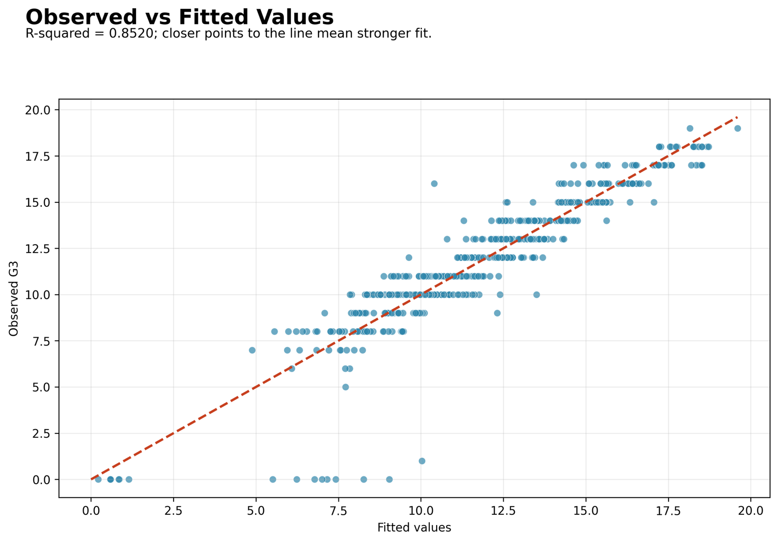
Most observations follow the equality direction through the central grade range, while several floor outcomes lie far below their predictions.
Multiple R = 0.923065 and R Squared = 0.852050 for 649 fitted observations.
Strong global agreement produces the high fit ratio, but the statistic averages across all squared deviations.
Cases 164 and 173 show that a high aggregate value can coexist with residuals near negative nine.
Python Chart 2: Residuals versus Fitted Values
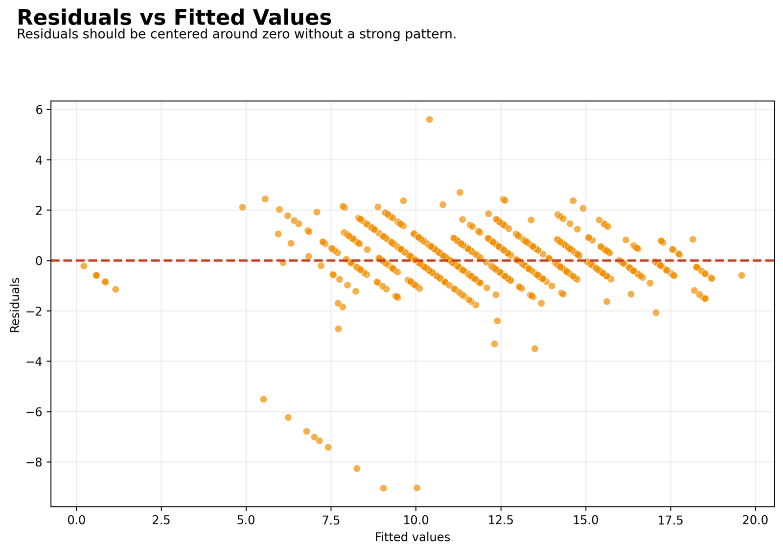
Residuals are centered broadly around zero, with integer-grade bands and an extended negative tail.
The squared residuals sum to SSE = 1000.626425; fitted RMSE = 1.241691.
Every vertical distance contributes to SSE and therefore determines the R Squared denominator reduction.
Fanning or curvature would qualify the linear fit even when the headline ratio remains high.
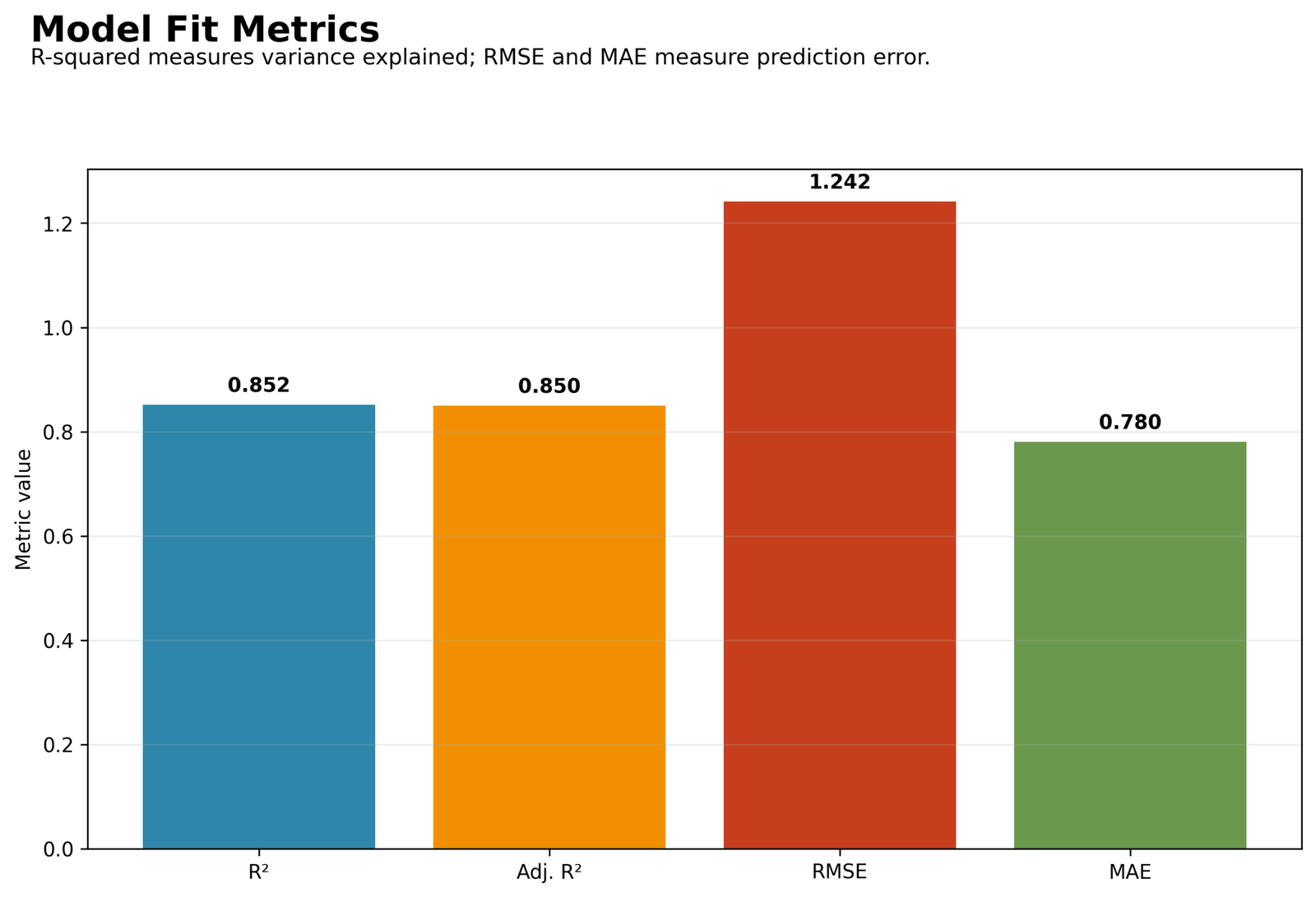
Python Chart 3: Model Summary
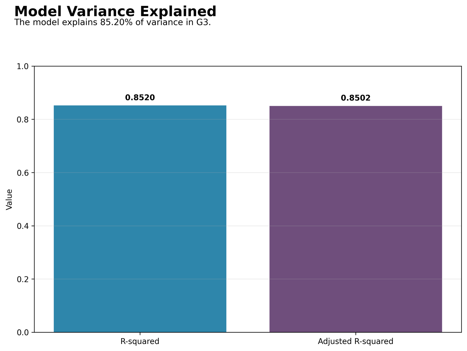
Ordinary and adjusted fit are close, while RMSE and MAE retain a different grade-point scale.
R Squared = 0.852050, adjusted = 0.850200, RMSE = 1.241691 and MAE = 0.780275.
The modest adjustment suggests the eight-parameter complexity charge is small relative to the fitted reduction in SSE.
Displaying error metrics prevents a variance ratio from being mistaken for grade-point accuracy.
Python Chart 4: Single-Predictor Fit Ranking
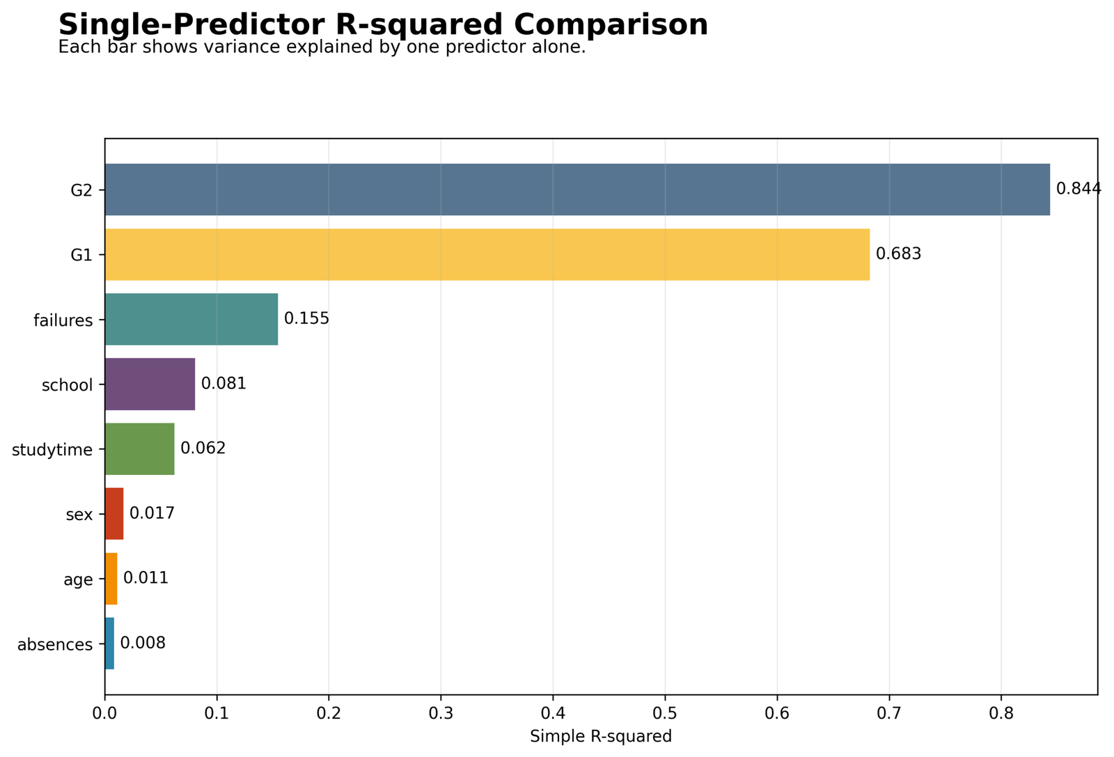
G2 dominates, G1 is second and every remaining single-predictor value is much smaller.
G2 = 0.843730, G1 = 0.682916, failures = 0.154697 and school = 0.080823.
These are separate models and contain overlapping variation. They cannot be added.
The graph shows why the complete 0.852050 value is driven mainly by prior-grade information.
Python Chart 5: Nested R Squared Change
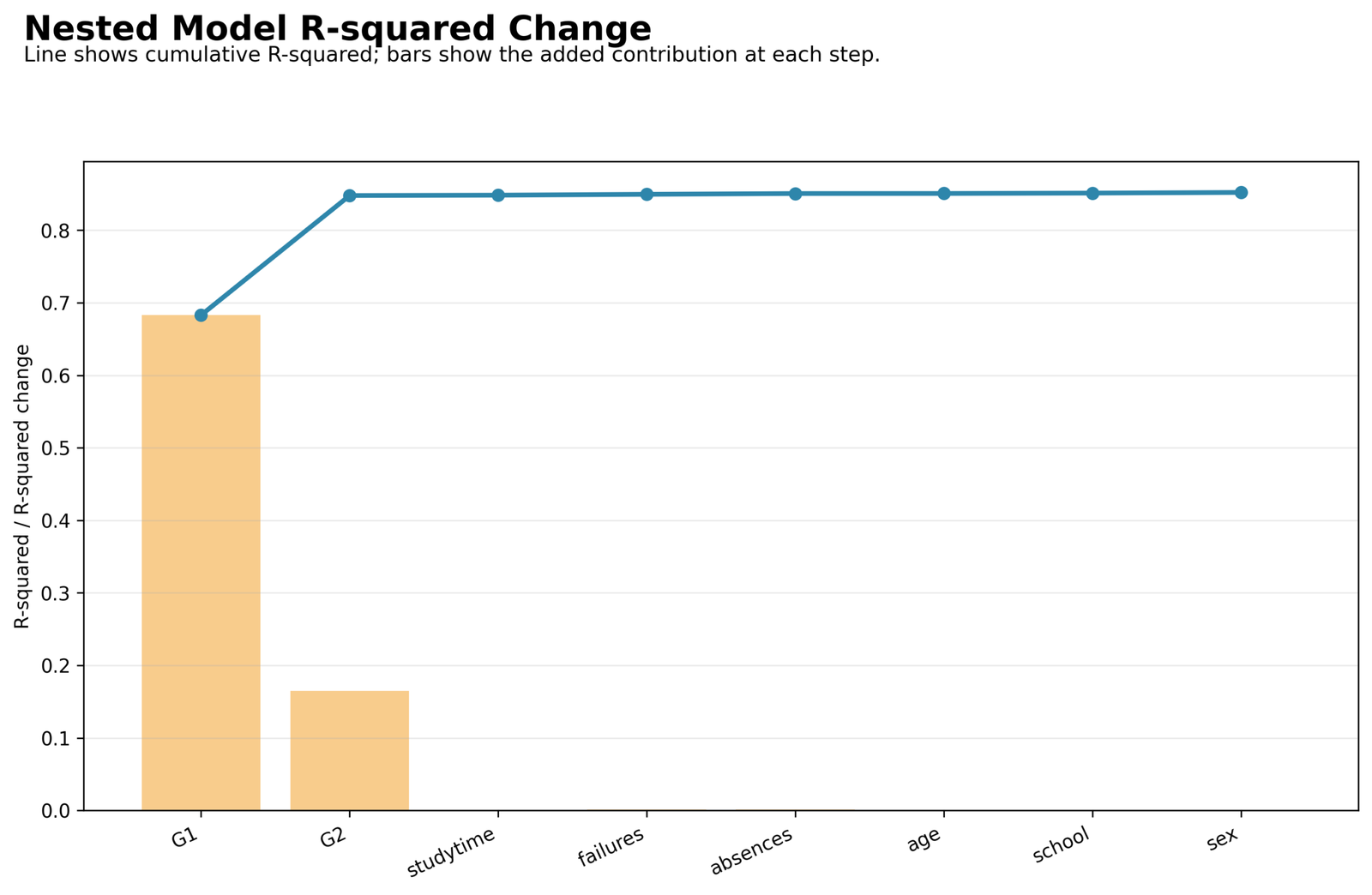
The sequence rises sharply for G1 and G2 and then flattens across the remaining six additions.
G2 adds 0.164846 after G1; age adds 0.000069; the final sex step adds 0.000892.
Sequential change measures conditional improvement at a particular entry position.
Statistical detectability must be read beside the size of the added fit.
Python Chart 6: Coefficients with Confidence Intervals
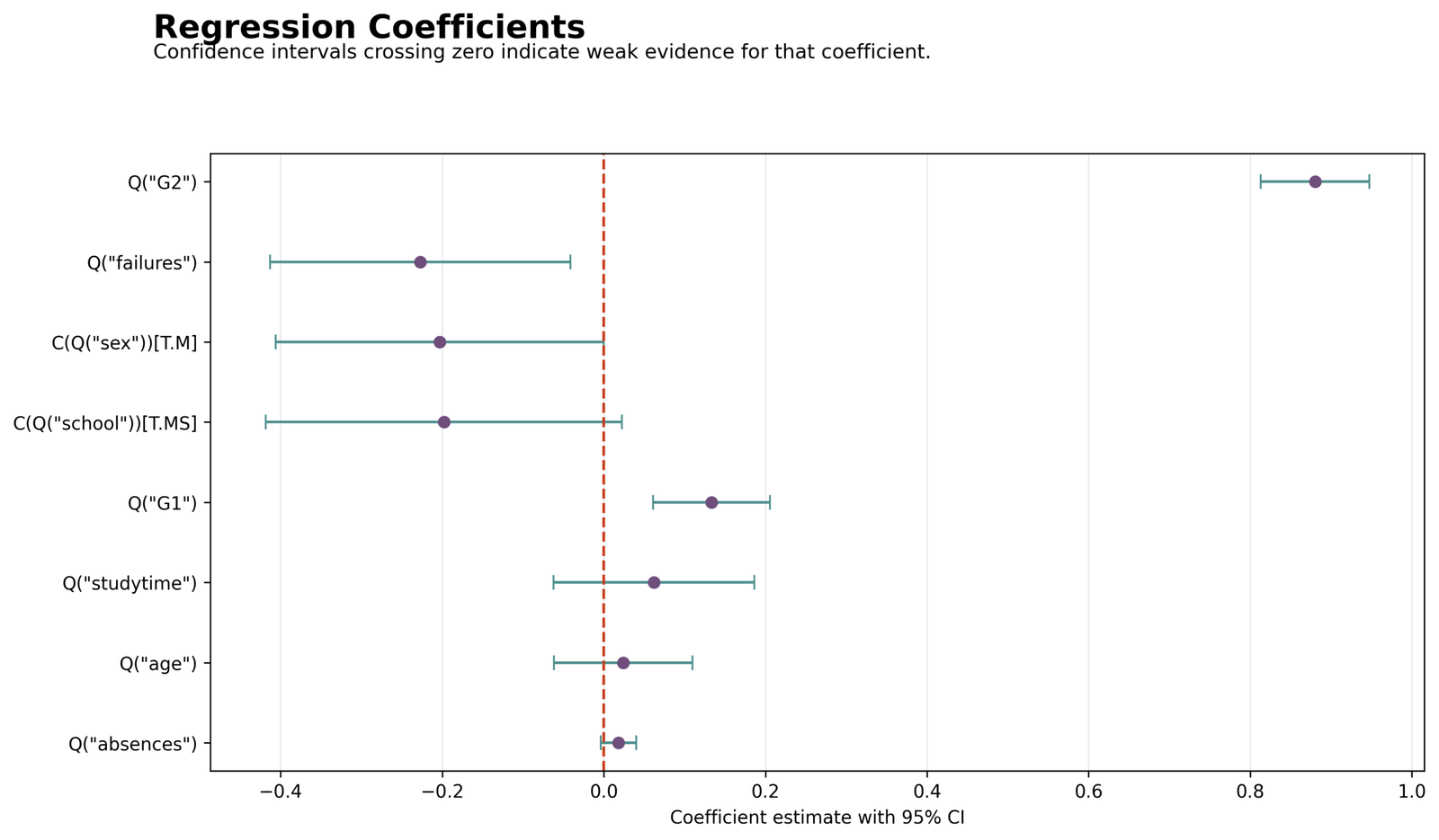
G2 has the largest positive slope. G1 is positive, failures is negative and several intervals cross zero.
G2 B = 0.880212 with CI [0.813188, 0.947237]; G1 B = 0.133173.
Coefficient direction and uncertainty do not divide or reconstruct the total R Squared.
The chart keeps model fit separate from term-specific estimates.
R Charts and Paired Explanations
The R visuals independently reproduce the same 649-row R Squared evidence and are arranged in two responsive pairs.
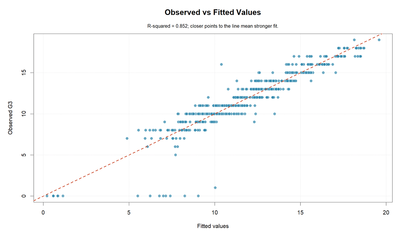
Observed versus Fitted
Pattern: The central grade cloud follows the identity direction.
Key values: R Squared = 0.852050 and multiple R = 0.923065.
Interpretation: The plot confirms strong aggregate alignment while retaining large individual misses.
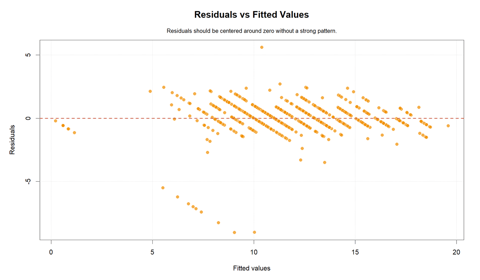
Residuals versus Fitted
Pattern: Errors center near zero with visible bands and a negative tail.
Key values: SSE = 1000.626425 and fitted RMSE = 1.241691.
Interpretation: The residual structure qualifies the global explained-variation statement.
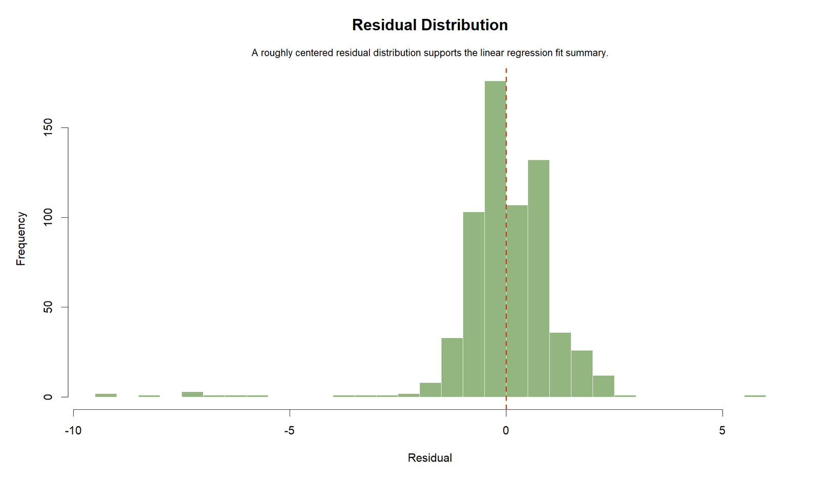
Residual Distribution
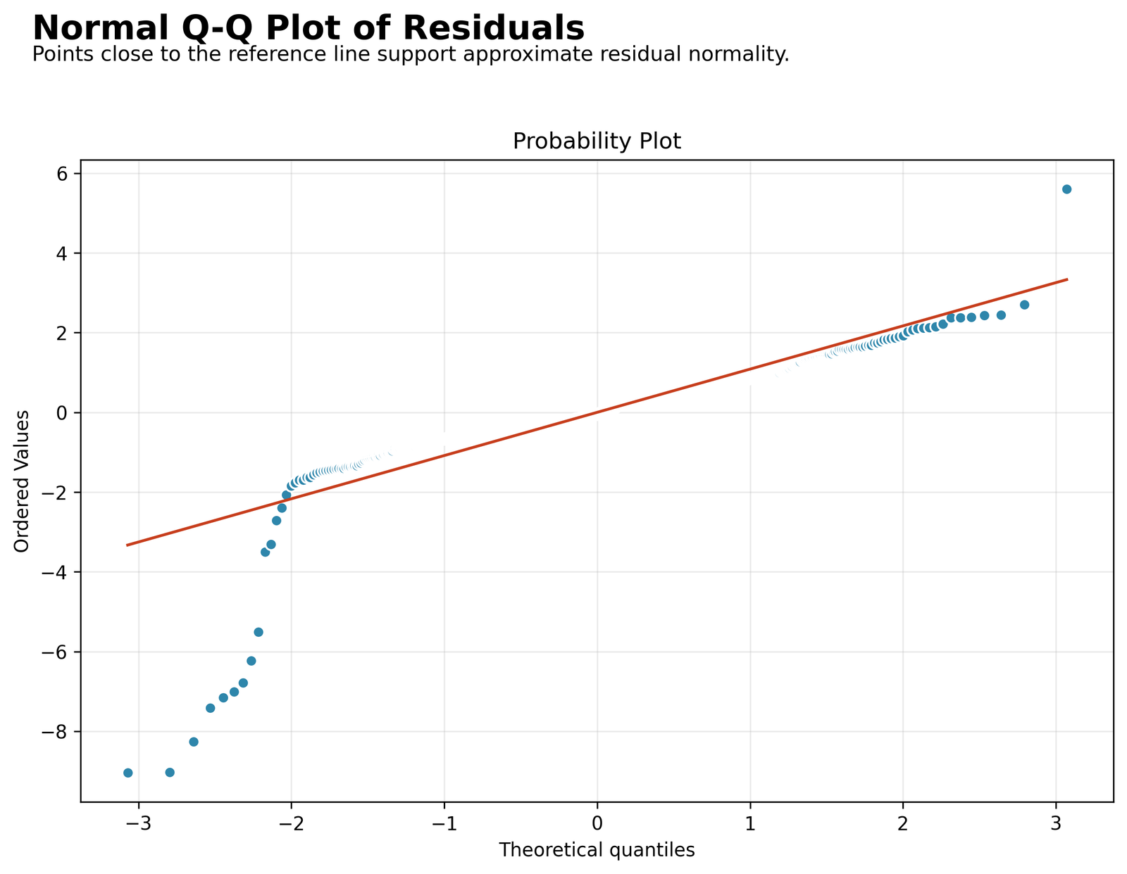
Pattern: Most residuals are modest but unusually large negative errors extend the lower tail.
Key values: Case 164 has standardized residual about −7.328003.
Interpretation: Strong R Squared does not guarantee normal or uniformly small errors.
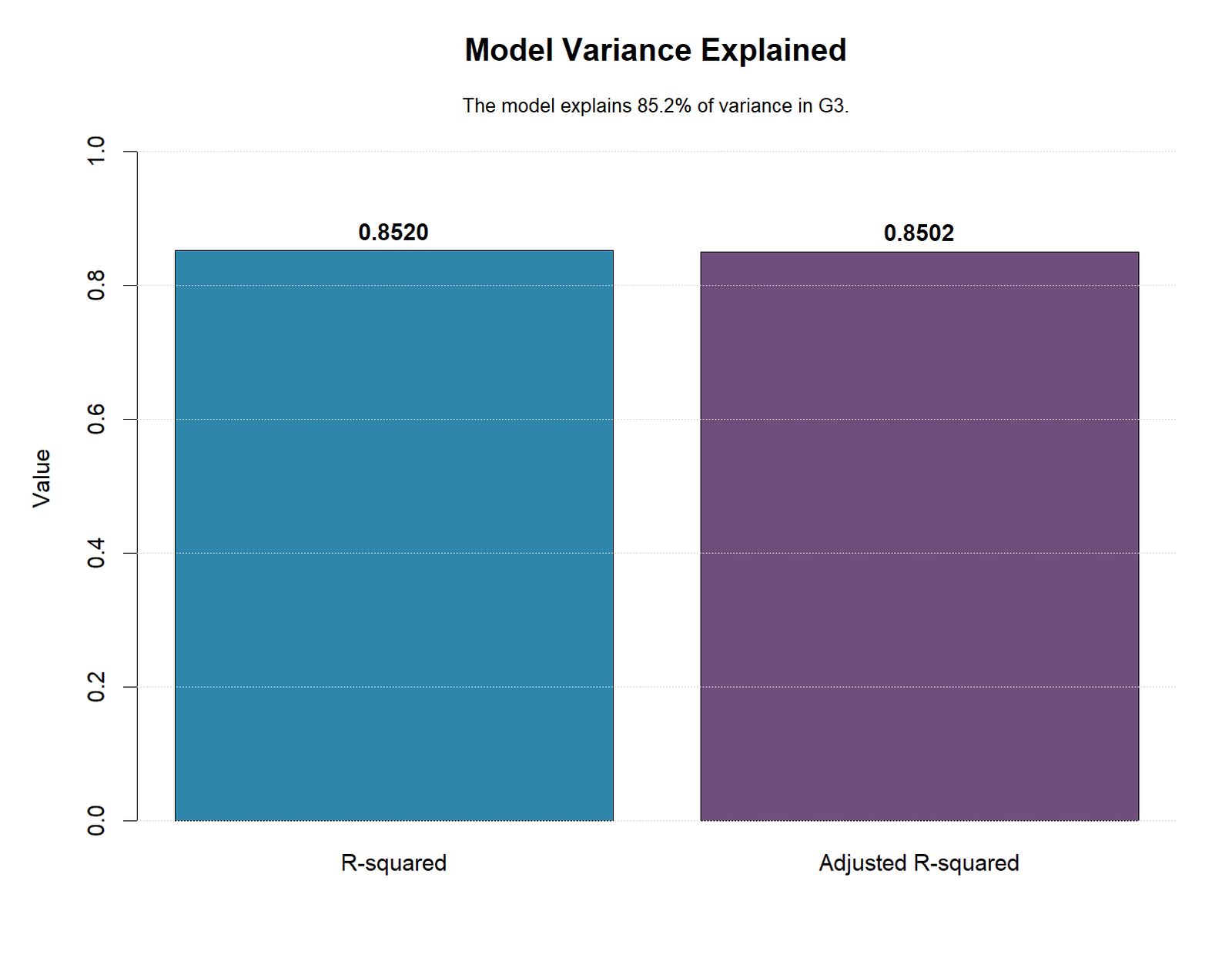
Model Summary
Pattern: Ordinary and adjusted fit remain close.
Key values: 0.852050, 0.850200, RMSE 1.241691 and MAE 0.780275.
Interpretation: The same evidence appears in proportional and outcome-unit metrics.
R Squared Coefficient and Parameter Interpretation
R Squared is a model-level measure. The coefficient table describes conditional slopes, reference-group contrasts and uncertainty. These two evidence layers should be connected but not merged.
G2 has B = 0.880212 and dominates both the conditional coefficient evidence and the single-predictor fit comparison. G1 remains positive at B = 0.133173 after G2 and the other six terms are included.
Failures has B = −0.227071. The male-versus-female indicator is −0.203144 with a confidence interval ending just below zero. School, studytime, absences and age have intervals crossing zero in the complete equation.
The complete R Squared cannot be assigned by reading coefficient sizes. G1 and G2 overlap strongly, and sequential change depends on entry order. Use partial, semi-partial, dominance or Shapley-style methods only when their distinct allocation question has been specified.
Predictions, Effects and Model Meaning
The 649 fitted values generate every residual used in SSE. Case 164 has observed G3 = 0, fitted G3 = 9.04254954986905, residual = −9.04254954986905, standardized residual = −7.328002959518951 and Cook distance = 0.15984364988462588.
Case 173 has observed G3 = 1, fitted G3 = 10.030661804035518 and residual = −9.030661804035518. These cases explain how the model can retain high R Squared while failing badly for particular floor outcomes.
The complete 649-row observed, fitted, residual, standardized-residual and Cook-distance ledger is preserved in the downloadable CSV supplied with this rewrite. It is intentionally excluded from the public HTML table layout so the article remains readable.
For new-data prediction, calculate fitted values without estimating the equation from those new outcomes. Then compute validation R Squared, RMSE and MAE. The current 0.852050 value describes the same sample used to estimate the coefficients.
R Squared Assumptions and Diagnostics
The eight-term linear equation and indicator coding must match the research question.
Linearity, spread, tail shape and influential errors require separate checks.
External or cross-validated predictions are required for predictive claims.
Linearity and Functional Form
A high R Squared does not prove the conditional mean is linear. Residual curvature can remain even when prior grades generate strong global agreement.
Homoscedasticity
Unequal residual spread does not change the arithmetic definition but affects classical standard errors and prediction intervals. Use residual plots and robust uncertainty when appropriate.
Residual Distribution
Normality is not required to compute the ratio. It matters for conventional small-sample inference. The supplied residual-distribution and Q-Q assets show why tail checks remain necessary.
Influence
Case 164 has the largest documented Cook distance, approximately 0.159844. It should be verified and examined through sensitivity analysis, not deleted automatically to improve fit.
Collinearity and Incremental Fit
G1 and G2 explain overlapping variation. High complete-model fit can coexist with unstable or modest additional coefficients for later terms.
Validation
Repeated or nested resampling should repeat all model-selection decisions. A validation R Squared can be lower or negative and is often more useful for deployment.
R Squared in Python, R, SPSS and Excel
Python
statsmodels supplies fitted values, residuals, coefficient tests, ANOVA evidence and influence diagnostics.
- Use one 649-row analysis frame.
- Reconstruct SST and SSE with NumPy.
- Export full-precision case evidence.
R
lm() and summary() provide ordinary and adjusted fit, while base influence functions reproduce the residual audit.
- Confirm factor references.
- Use
model.frame(fit). - Export the same observed and fitted rows.
SPSS
The Model Summary and ANOVA tables report R, R Square, adjusted R Square, standard error and the global F test.
- Create explicit school and sex indicators for REGRESSION.
- Save predicted, residual and Cook variables.
- Report Sig. .000 as p < .001.
Excel
A spreadsheet can independently verify the complete variance identity from observed and fitted columns.
- Calculate SST and SSE separately.
- Use full-precision fitted values.
- Distinguish RMSE from residual standard error.
Code and Formula Panels
Python R Squared verification workflow
from pathlib import Path
import numpy as np
import pandas as pd
import statsmodels.formula.api as smf

DATA = Path("dataset.csv")
OUTCOME = "G3"
FORMULA = (
    'Q("G3") ~ Q("G1") + Q("G2") + Q("studytime") + '
    'Q("failures") + Q("absences") + Q("age") + '
    'C(Q("school")) + C(Q("sex"))'
)

raw = pd.read_csv(DATA)
needed = ["G3", "G1", "G2", "studytime", "failures", "absences", "age", "school", "sex"]
dat = raw[needed].dropna().copy()
fit = smf.ols(FORMULA, data=dat).fit()

y = fit.model.endog
fitted = fit.fittedvalues.to_numpy()
resid = fit.resid.to_numpy()
y_bar = y.mean()

sst = np.sum((y - y_bar) ** 2)
sse = np.sum(resid ** 2)
ssr = sst - sse
r_squared = 1 - sse / sst
adjusted_r_squared = 1 - (1 - r_squared) * (len(y) - 1) / fit.df_resid
rmse = np.sqrt(sse / len(y))
residual_standard_error = np.sqrt(sse / fit.df_resid)
mae = np.mean(np.abs(resid))

print({
    "n": int(fit.nobs),
    "r_squared": r_squared,
    "adjusted_r_squared": adjusted_r_squared,
    "sst": sst,
    "ssr": ssr,
    "sse": sse,
    "rmse": rmse,
    "residual_standard_error": residual_standard_error,
    "mae": mae,
    "f_statistic": fit.fvalue,
    "model_p_value": fit.f_pvalue,
})

influence = fit.get_influence()
case_audit = dat.copy()
case_audit["observed"] = y
case_audit["fitted"] = fitted
case_audit["residual"] = resid
case_audit["standardized_residual"] = influence.resid_studentized_internal
case_audit["cooks_distance"] = influence.cooks_distance[0]
case_audit.to_csv("r_squared_case_audit.csv", index=False)
R R Squared verification workflow
dat <- read.csv("dataset.csv", check.names = FALSE)
needed <- c("G3", "G1", "G2", "studytime", "failures", "absences", "age", "school", "sex")
model_dat <- dat[complete.cases(dat[needed]), needed]

fit <- lm(
  G3 ~ G1 + G2 + studytime + failures + absences + age + school + sex,
  data = model_dat
)

y <- model.response(model.frame(fit))
fitted_values <- fitted(fit)
residual_values <- residuals(fit)

sst <- sum((y - mean(y))^2)
sse <- sum(residual_values^2)
ssr <- sst - sse
r_squared <- 1 - sse / sst
adjusted_r_squared <- summary(fit)$adj.r.squared
rmse <- sqrt(mean(residual_values^2))
residual_standard_error <- summary(fit)$sigma
mae <- mean(abs(residual_values))

model_summary <- data.frame(
  n = nobs(fit),
  r_squared = r_squared,
  adjusted_r_squared = adjusted_r_squared,
  sst = sst,
  ssr = ssr,
  sse = sse,
  rmse = rmse,
  residual_standard_error = residual_standard_error,
  mae = mae,
  f_statistic = unname(summary(fit)$fstatistic[1]),
  df_model = unname(summary(fit)$fstatistic[2]),
  df_residual = unname(summary(fit)$fstatistic[3])
)

case_audit <- transform(
  model.frame(fit),
  observed = y,
  fitted = fitted_values,
  residual = residual_values,
  standardized_residual = rstandard(fit),
  cooks_distance = cooks.distance(fit)
)

write.csv(model_summary, "r_squared_model_summary.csv", row.names = FALSE)
write.csv(case_audit, "r_squared_case_audit.csv", row.names = FALSE)
print(model_summary)
SPSS R Squared syntax and residual audit
* R Squared worked model: G3 from six numeric predictors and two indicators.

UNIANOVA G3 BY school sex WITH G1 G2 studytime failures absences age
 /METHOD=SSTYPE(3)
 /INTERCEPT=INCLUDE
 /PRINT=PARAMETER DESCRIPTIVE ETASQ OPOWER HOMOGENEITY
 /CRITERIA=ALPHA(.05)
 /DESIGN=G1 G2 studytime failures absences age school sex.

* Equivalent REGRESSION requires explicit dummy variables.
* GP is the school reference and female is the sex reference.
COMPUTE school_MS = (school = "MS").
COMPUTE sex_M = (sex = "M").
EXECUTE.

REGRESSION
 /MISSING LISTWISE
 /STATISTICS COEFF OUTS R ANOVA CHANGE CI(95) COLLIN TOL
 /DEPENDENT G3
 /METHOD=ENTER G1 G2 studytime failures absences age school_MS sex_M
 /SAVE PRED(rsq_pred) RESID(rsq_resid) ZRESID(rsq_zresid) COOK(rsq_cook).

* Reconstruct SSE from saved residuals.
COMPUTE rsq_sq_resid = rsq_resid ** 2.
DESCRIPTIVES VARIABLES=rsq_pred rsq_resid rsq_zresid rsq_cook rsq_sq_resid
 /STATISTICS=MEAN STDDEV MIN MAX SUM.
Excel R Squared formulas
Assume each data row contains:
Observed G3, fitted G3, and the observed G3 mean.

Residual
=ObservedCell-FittedCell

Squared residual
=ResidualCell^2

Deviation from observed mean
=ObservedCell-AVERAGE(ObservedRange)

Squared deviation from observed mean
=DeviationCell^2

SSE
=SUM(SquaredResidualRange)

SST
=SUM(SquaredDeviationRange)

SSR
=SSTCell-SSECell

R Squared
=1-SSECell/SSTCell

Adjusted R Squared
=1-(1-RSquaredCell)*(NCell-1)/(NCell-PredictorCountCell-1)

Multiple R for a model with an intercept
=SQRT(MAX(0,RSquaredCell))

F statistic
=(RSquaredCell/PredictorCountCell)/((1-RSquaredCell)/(NCell-PredictorCountCell-1))

Global model p-value
=F.DIST.RT(FStatisticCell,PredictorCountCell,NCell-PredictorCountCell-1)

Fitted RMSE using N
=SQRT(SSECell/NCell)

Residual standard error using residual degrees of freedom
=SQRT(SSECell/(NCell-PredictorCountCell-1))

MAE
=AVERAGE(AbsoluteResidualRange)
Advanced R Squared Topics
These 26 panels extend the worked R Squared analysis from arithmetic identity to model comparison, validation and deployment.
1. R Squared Estimand
R Squared is the fraction of observed outcome sum-of-squares variation accounted for by fitted values from one declared model on one declared sample.
It is an in-sample descriptive ratio unless the predictions come from validation data. The number does not identify causal contributions and does not equal the proportion of individual outcomes predicted correctly.
2. Variance Identity
With an intercept and ordinary least squares on identical rows, SST decomposes into SSR plus SSE. The worked values are 6763.266564 = 5762.640139 + 1000.626425.
Reconstructing the identity is a strong audit because it checks the observed mean, fitted values and residual ledger independently of a software label.
3. Intercept Requirement
The familiar bounded zero-to-one interpretation assumes a model with an intercept and compares fitted error with an intercept-only baseline.
Without an intercept, the usual decomposition can fail and R Squared can behave differently. The model specification must therefore be reported with the statistic.
4. Why R Squared Can Be Negative
On new validation data, predictions can produce more squared error than simply using the validation outcome mean. The resulting out-of-sample R Squared can be negative.
A negative validation value is meaningful: the tested prediction rule performs worse than the stated mean benchmark for those observations.
5. Adjusted R Squared
Adjusted R Squared penalizes the ordinary ratio for estimating additional predictor parameters. It rises only when the added fit is large enough relative to the complexity charge.
The worked value falls from 0.852050 to 0.850200, a small difference because the model gain is large relative to eight fitted predictor parameters and 649 observations.
6. Multiple R
For an intercept model with nonnegative R Squared, multiple R is the positive square root of R Squared. Here it equals 0.923065.
It is the correlation between observed and fitted values in this setting. It is not a standardized regression coefficient and should not be interpreted as the contribution of one predictor.
7. R Squared and RMSE
R Squared standardizes error by the observed outcome dispersion, whereas RMSE remains in G3 grade points.
Two studies can have similar R Squared but different practical error because their outcome ranges and residual scales differ. Both metrics are required.
8. Fitted RMSE versus Residual Standard Error
The supplied RMSE is sqrt(SSE/N) = 1.241691. Residual standard error uses residual degrees of freedom and equals approximately 1.250391.
The quantities are close but not identical. A careful report labels the denominator rather than calling every square-root error RMSE.
9. R Squared and MAE
MAE = 0.780275 gives the average absolute fitted error and is less sensitive to a few very large residuals than RMSE.
The gap between RMSE and MAE reflects tail errors such as cases 164 and 173. R Squared alone hides that error-shape information.
10. Nested R Squared Change
A nested change compares a reduced model with a full model fitted to the same outcome rows. The increase is conditional on the predictors already entered.
G2 adds 0.164846 after G1, while age adds only 0.000069 at its position. Entry order therefore defines the sequential change interpretation.
11. F-Change Test
The F-change test evaluates whether the added parameter block reduces SSE more than expected under the reduced-model null.
A detectable change can still be substantively tiny. The final sex step adds only 0.000892 even though its change-test p-value is approximately 0.049871.
12. Sequential versus Partial Contributions
Sequential increments depend on entry order. Partial or semi-partial measures answer different conditional questions and should not be silently substituted.
The worked nested sequence is explicitly G1, G2, studytime, failures, absences, age, school and sex. Reordering the terms redistributes the changes.
13. Single-Predictor Fit
G2 alone produces R Squared = 0.843730 and G1 alone produces 0.682916. These are separate one-predictor models.
Their values cannot be added because G1 and G2 explain overlapping outcome variation. The full model does not divide its 0.852050 equally among predictors.
14. Categorical Predictor Coding
school and sex enter as indicator variables with GP and female as the reference groups. One fitted parameter is used for each binary factor.
Changing references changes coefficient signs and labels but does not change fitted values or the complete-model R Squared when the same factor information is retained.
15. Comparing Models
Ordinary R Squared never decreases when predictors are added to an OLS model fitted to the same rows with an intercept.
A higher value therefore does not automatically identify the better model. Use adjusted fit, validation error, theory and parsimony when specifications differ.
16. Comparing Different Samples
R Squared values should not be ranked directly when models use different outcome rows, transformations or populations.
SST changes with the sample. A larger ratio can reflect a narrower or easier outcome distribution rather than a genuinely better prediction rule.
17. Outcome Transformations
Transforming G3 changes the variance scale and therefore the meaning of R Squared. A model for log outcome variation answers a different question from a model for raw grade variation.
Back-transformed prediction performance should be reported on the scale relevant to decisions rather than relying only on transformed-scale fit.
18. Nonlinear Models and Pseudo R Squared
Logistic, count and survival models do not generally share the OLS sum-of-squares identity. Their pseudo R Squared measures use likelihood or other definitions.
Pseudo values should be named by formula and should not be interpreted as the percentage of raw outcome variance explained.
19. Out-of-Sample R Squared
Validation R Squared should be computed from predictions generated without using the validation outcomes for fitting or model selection.
The current 0.852050 value is fitted-sample evidence. It should not be presented as external predictive performance.
20. Cross-Validated R Squared
Cross-validation generates held-out predictions across folds and can summarize predictive performance more realistically than fitted R Squared.
All preprocessing and variable selection must occur within each training fold. Otherwise the cross-validated value remains optimistic.
21. Influential Cases
Case 164 has residual about -9.042550, standardized residual about -7.328003 and Cook distance about 0.159844. Case 173 has a similarly large negative residual.
These observations do not erase strong global fit, but they show that aggregate explained variation can coexist with serious individual errors.
22. Residual Assumptions
R Squared is arithmetically defined even when residuals are nonnormal or heteroscedastic, but inferential claims and prediction intervals still depend on model conditions.
Residual-versus-fitted and distribution checks must accompany the headline ratio. A large value is not a diagnostic certificate.
23. Collinearity
Strong overlap among predictors can leave total R Squared high while individual coefficients become unstable or uncertain.
The dominance of prior grades means the full model can predict well even when small additional slopes are sensitive to specification choices.
24. Overfitting
Adding flexible terms can raise fitted R Squared by absorbing sample noise. The monotonic property makes training fit a weak model-selection criterion by itself.
Use validation, adjusted fit or prespecified nested tests. The intended use and feature availability should guide the final equation.
25. Availability at Prediction Time
G2 is measured close to final G3 and accounts for most of the fitted variation. A model intended for early intervention may not have G2 available.
High R Squared does not make a temporally unavailable predictor suitable for deployment. Report the prediction time and feature availability.
26. R Squared Decision Framework
Define the outcome scale, model formula, sample and purpose. Reconstruct SST, SSE and SSR; report ordinary and adjusted fit; then add RMSE, MAE, nested changes and diagnostics.
For prediction claims, replace fitted values with protected validation predictions. For explanatory claims, avoid allocating the total ratio causally among correlated predictors.
APA-Style Reporting
A multiple linear regression predicted final grade G3 from G1, G2, studytime, failures, absences, age, school and sex for 649 complete observations. The model was statistically significant, F(8, 640) = 460.72, p < .001, R² = .852, adjusted R² = .850. The model residual sum of squares was 1000.63 compared with total sum of squares 6763.27. Fitted RMSE was 1.24 grade points and MAE was 0.78. G2 supplied the largest declared nested increment after G1, ΔR² = .165. Residual and influence checks identified several large negative errors, including case 164, so the strong fitted R Squared was not interpreted as uniform individual accuracy or external validation.
Publication Checklist
- State G3 as the outcome.
- List all eight predictor parameters.
- Report 649 complete records.
- State that the model includes an intercept.
- Report SST, SSR and SSE.
- Reconstruct R Squared arithmetically.
- Report adjusted R Squared.
- Distinguish RMSE from residual standard error.
- Report MAE in grade points.
- State the nested entry order.
- Report change magnitude beside p-values.
- Do not add single-predictor fit values.
- Identify school and sex references.
- Review residual and Q-Q evidence.
- Review cases 164 and 173.
- Keep fitted and validation fit separate.
- Verify all chart and report URLs.
- Retain five advertisement placements.
Downloads and Verification Resources
Frequently Asked Questions
What is R Squared?
R Squared is one minus the ratio of residual sum of squares to total sum of squares for the declared outcome, sample and model. In the worked model it equals 0.8520498318760341.
Does R Squared mean prediction accuracy?
No. It describes proportional sum-of-squares reduction relative to an intercept-only baseline. RMSE, MAE and validation performance describe prediction error more directly.
What does 0.852050 mean here?
The fitted eight-predictor equation accounts for about 85.205% of observed in-sample G3 sum-of-squares variation.
Why is adjusted R Squared lower?
It applies a complexity charge for eight predictor parameters. The adjusted value is 0.8502004547744846.
Can R Squared decrease when predictors are added?
Training R Squared for nested OLS models with an intercept cannot decrease. Adjusted or validation R Squared can decrease.
What is multiple R?
Here it is sqrt(0.8520498318760341) = 0.9230654537333927, the positive observed-versus-fitted correlation for the intercept model.
Which predictor has the largest single-predictor fit?
G2, with R Squared = 0.8437304348447063. G1 is second at 0.6829156800171083.
Can single-predictor values be added?
No. Predictors explain overlapping outcome variation, especially G1 and G2.
What is the largest nested increment?
G2 adds 0.16484585367188342 after G1 in the declared sequence.
Is the final sex increment important?
It adds 0.0008924164040048366. Its change-test p-value is near 0.05, but the magnitude is very small.
What is the difference between RMSE and residual standard error?
Fitted RMSE uses N and equals 1.241691. Residual standard error uses 640 residual degrees of freedom and is about 1.250391.
Can R Squared be negative?
Yes on validation data or under some no-intercept definitions. It means the predictions are worse than the stated mean benchmark.
Does a high value prove linearity or normal residuals?
No. The residual and Q-Q evidence must be examined separately.
Why preserve the case-level CSV?
The 649 rows reproduce SSE and reveal influential errors that a single ratio hides.
Can logistic or Cox models use the same interpretation?
No. Those models usually report named pseudo R Squared or discrimination measures, not the OLS variance identity.
How can Excel verify the result?
Calculate observed-minus-fitted residuals for SSE, observed-minus-mean deviations for SST, square and sum both columns, then compute 1 minus SSE divided by SST.
R Squared Conclusion
The verified eight-predictor model has R Squared = 0.8520498318760341 and adjusted R Squared = 0.8502004547744846. Its 649 residual squares sum to 1000.6264252027902, while total G3 sum of squares is 6763.2665639445295.
G2 accounts for most of the stand-alone fitted variation and creates the largest nested increase after G1. Later predictors add comparatively little, even when an individual change test crosses a conventional threshold.
RMSE = 1.241691 and MAE = 0.780275 keep error in grade-point units. Cases 164 and 173 demonstrate that strong global fit can coexist with serious individual misses.
The defensible conclusion is that this exact equation represents most observed in-sample G3 variation. It does not establish causal allocation, uniform accuracy or future performance without protected validation.