Ansari–Bradley Test: Formula, Assumptions, Worked Example, Python, R, SPSS, SAS and Excel Guide
The Ansari–Bradley test compares the scale or dispersion of two independent populations without requiring normality. This evidence-first guide analyses G3 final grades for 649 students by family educational support, audits the equal-location condition, reconstructs the symmetric-score statistic, reconciles asymptotic and deterministic permutation results, and verifies the analysis across Python, R, SPSS, SAS and Excel.
251 without support
398 with support
Both medians = 12
A = 40,094.5
p = .5183
Ansari–Bradley Test Model Overview
The Ansari–Bradley test is a rank-based procedure for comparing the scale parameters of two independent groups. In practical terms, scale describes how tightly observations cluster around a common location. The method does not compare the group means, does not test whether the medians differ, and does not ask whether every feature of the two distributions is identical. It asks a narrower question: after the groups have a defensible common location, is one population systematically more dispersed than the other?
The worked analysis compares final grade G3 between students whose family educational support variable famsup is coded no and yes. The group medians are both 12 and the interquartile ranges are both 4, providing a favourable starting point for a scale-focused test. Nevertheless, the unsupported group has a larger standard deviation, 3.6022 versus 2.9674, and a larger variance, 12.9756 versus 8.8052. The formal analysis determines whether that descriptive difference is large relative to the sampling variation in the Ansari–Bradley score sum.
Quick Answer: Ansari–Bradley Test Result
Statistical Decision
- Null hypothesis: the population scale ratio equals 1.
- Alternative: the scale ratio differs from 1.
- Alpha: .05.
- Decision: fail to reject H0.
- Evidence: asymptotic and permutation results agree.
Substantive Meaning
- Both group medians are 12.
- Both group IQRs are 4.
- The no-support SD is descriptively 21.39% larger.
- The variance ratio is 1.4736.
- The formal scale evidence remains weak, |z|/√N = 0.0254.
Table of Contents
- Research question and hypotheses
- When to use the test
- Assumption and validity gate
- Variables and analysis design
- Descriptive data audit
- Distribution forensics
- How symmetric scores work
- Formula and manual calculation
- Ties, exact and permutation inference
- Complete results
- Data discussion and interpretation
- Robustness and sensitivity
- Python chart stories
- R verification gallery
- Software workflows
- Expandable code
- Cross-software reconciliation
- Related-test comparison
- APA reporting
- Common mistakes
- Practice questions
- Downloads
- Related guides
- Frequently asked questions
- Conclusion
Research Question, Hypotheses and Direction
Research Question
Do the population distributions of G3 have different scale parameters for students without and with family educational support, given a defensible common location?
| Component | Formal statement | Interpretation |
|---|---|---|
| Null hypothesis | H0: s = 1 | The two populations have the same scale parameter. |
| Two-sided alternative | H1: s ≠ 1 | The population scales differ in either direction. |
| Directional convention | Smaller A for sample X | More sample-X observations occupy the pooled extremes, consistent with larger X scale. |
| Current focal sample | X = famsup no | The reported A statistic sums symmetric scores for the no-support group. |
The two-sided alternative was prespecified. A one-sided conclusion should not be selected after seeing that the unsupported group has the larger sample standard deviation. Directional testing requires a defensible prior scientific hypothesis.
When to Use the Ansari–Bradley Test
If observations are paired or repeated, choose a paired procedure instead.
If the scientific question is location, do not substitute a scale test.
Inspect medians and distribution shapes before interpreting the result as scale.
Strong Use Case
- Two independent samples.
- Numeric or meaningfully ordered outcome.
- Non-normality, outliers or heavy tails make a normal-theory variance test unattractive.
- A common median or aligned location is scientifically defensible.
- The primary question concerns dispersion.
Choose Another Method When
- Three or more groups require a k-sample scale test.
- Medians differ materially.
- The research question concerns general distribution equality.
- Observations are clustered or weighted.
- The outcome contains only a few unordered categories.
Research Question to Method Map
| Question | Preferred starting method | Why |
|---|---|---|
| Two independent groups: central tendency | Mann–Whitney, Brunner–Munzel or a robust location model | Targets location or stochastic ordering rather than scale. |
| Two independent groups: scale only | Ansari–Bradley, Mood or Siegel–Tukey | Uses rank scores designed for dispersion differences. |
| Three or more groups: robust spread | Fligner–Killeen or Brown–Forsythe | Extends scale comparison beyond two groups. |
| Normal two-group variance comparison | F test | Directly targets a variance ratio under normality. |
| Simultaneous location and scale | Lepage-type procedure or separate prespecified tests | A single scale test cannot identify both components. |
The selection step is essential. Calling every rank-based procedure “a nonparametric alternative to the t test” is incorrect. The Ansari–Bradley score pattern is intentionally sensitive to observations at the pooled extremes.
Assumption and Validity Gate
A nonparametric label does not mean assumption-free. The result is meaningful only when the study design and distributional conditions support a scale interpretation.
Independent Observations — Pass
Each of the 649 students contributes one G3 value to one family-support group. The analysis does not reuse students across groups.
Exactly Two Groups — Pass
famsup contains the two analysed levels, no and yes, with n = 251 and n = 398.
Common Median — Supported
Both sample medians equal 12. The central 50% also spans 10 to 14 in both groups.
Comparable Shape — Review
The unsupported group is more negatively skewed and has more zero grades. The ECDF and frequency tables therefore belong in the interpretation.
Ties — Explicitly Corrected
G3 is integer-valued, creating many tied ranks. The asymptotic variance is tie-adjusted and the result is checked by permutation.
Sampling and Causality — Limited
The observed association does not show that family support causes a change in dispersion. Generalisation depends on the sampling design.
Assumption Audit Table
| Condition | Observed evidence | Judgment | Reporting implication |
|---|---|---|---|
| Independence | One row per student; mutually exclusive groups | Reasonable | Use a two-sample procedure. |
| Common location | Median 12 in both groups; Q1 = 10 and Q3 = 14 in both | Supported descriptively | Scale interpretation is defensible. |
| Similar distribution family | Both concentrate around 10–14, but tail weights differ | Approximate, not perfect | Discuss tails and skewness rather than claiming pure rescaling. |
| Continuity | G3 is discrete integer data with extensive ties | Not met literally | Use tie correction and permutation verification. |
| Random sampling | Not established by the statistical output | Unknown | Avoid causal or population-wide claims. |
Variables, Coding and Analysis Specification
| Variable | Role | Coding | Valid N | Purpose |
|---|---|---|---|---|
| student_id | Record identifier | 1–649 | 649 | Confirms one row per student. |
| G3 | Numeric outcome | Observed 0–19 | 649 | Final grade whose scale is compared. |
| famsup | Grouping variable | no / yes | 649 | Defines the two independent samples. |
| Sample X | Focal score-sum group | famsup = no | 251 | Its symmetric scores are summed to form A. |
| Sample Y | Comparison group | famsup = yes | 398 | Completes the pooled reference distribution. |
Reproducible Analysis Statement
G3 was analysed as a numeric outcome and family educational support (famsup) as a two-level independent grouping variable. The no-support group was designated sample X. The analysis used a two-sided Ansari–Bradley test, midranks for tied G3 values, a tie-adjusted asymptotic variance and a deterministic 10,000-permutation robustness check.
Descriptive Data Audit Before the Test
The formal statistic should never be interpreted without first locating the descriptive difference. Here the centre of the two groups is nearly identical, while the tail behaviour differs more than the middle 50%.
| Statistic | famsup = no | famsup = yes | No − yes | Analytical meaning |
|---|---|---|---|---|
| N | 251 | 398 | −147 | The groups are unbalanced but both are large. |
| Mean | 11.6653 | 12.0578 | -0.3925 | Location is close; the test is not about this difference. |
| 5% trimmed mean | 11.9471 | 12.1139 | -0.1668 | Removing tail observations narrows the mean difference. |
| Median | 12.0000 | 12.0000 | 0 | Supports the common-location requirement. |
| Q1 | 10.0000 | 10.0000 | 0 | Lower quartiles match. |
| Q3 | 14.0000 | 14.0000 | 0 | Upper quartiles match. |
| IQR | 4.0000 | 4.0000 | 0 | Central dispersion is identical descriptively. |
| Standard deviation | 3.6022 | 2.9674 | 0.6348 | The unsupported group looks more dispersed. |
| Variance | 12.9756 | 8.8052 | 4.1703 | Descriptive variance ratio = {variance_ratio:.4f}. |
| Skewness | -1.188 | -0.519 | -0.669 | The no-support distribution has a heavier lower tail. |
| Excess kurtosis | 2.776 | 1.926 | 0.850 | Tail concentration differs descriptively. |
For interpretation of these summaries, see descriptive statistics, standard deviation, variance and the interquartile range.
Distribution Forensics: Where the Apparent Spread Difference Comes From
The complete frequency table shows that both groups concentrate between G3 = 10 and G3 = 14. The main imbalance appears at the lower extreme rather than throughout the entire distribution.
| G3 | No count | No % | Yes count | Yes % | Total |
|---|---|---|---|---|---|
| 0 | 11 | 4.38% | 4 | 1.01% | 15 |
| 1 | 0 | 0.00% | 1 | 0.25% | 1 |
| 2 | 0 | 0.00% | 0 | 0.00% | 0 |
| 3 | 0 | 0.00% | 0 | 0.00% | 0 |
| 4 | 0 | 0.00% | 0 | 0.00% | 0 |
| 5 | 1 | 0.40% | 0 | 0.00% | 1 |
| 6 | 1 | 0.40% | 2 | 0.50% | 3 |
| 7 | 4 | 1.59% | 6 | 1.51% | 10 |
| 8 | 8 | 3.19% | 27 | 6.78% | 35 |
| 9 | 18 | 7.17% | 17 | 4.27% | 35 |
| 10 | 39 | 15.54% | 58 | 14.57% | 97 |
| 11 | 38 | 15.14% | 66 | 16.58% | 104 |
| 12 | 28 | 11.16% | 44 | 11.06% | 72 |
| 13 | 26 | 10.36% | 56 | 14.07% | 82 |
| 14 | 27 | 10.76% | 36 | 9.05% | 63 |
| 15 | 21 | 8.37% | 28 | 7.04% | 49 |
| 16 | 12 | 4.78% | 24 | 6.03% | 36 |
| 17 | 11 | 4.38% | 18 | 4.52% | 29 |
| 18 | 5 | 1.99% | 10 | 2.51% | 15 |
| 19 | 1 | 0.40% | 1 | 0.25% | 2 |
| 20 | 0 | 0.00% | 0 | 0.00% | 0 |
Tail and Centre Audit
| Region | No group | Yes group | Interpretation |
|---|---|---|---|
| G3 = 0 | 11 / 251 = 4.38% | 4 / 398 = 1.01% | The unsupported group contributes most of the extreme lower tail. |
| G3 < 8 | 17 / 251 = 6.77% | 13 / 398 = 3.27% | Low grades are proportionally more common without support. |
| G3 = 10–14 | 158 / 251 = 62.95% | 260 / 398 = 65.33% | The central grade region is very similar. |
| G3 ≥ 17 | 17 / 251 = 6.77% | 29 / 398 = 7.29% | The upper tail is proportionally similar. |
| Q1 to Q3 | 10 to 14 | 10 to 14 | The middle half has the same observed width. |
Why the SDs Differ
Standard deviation gives substantial weight to observations far from the mean. The eleven zeros in the no-support group increase its variance even though both groups have the same median and IQR.
Why the Test Is Still Nonsignificant
The Ansari–Bradley statistic evaluates the complete pooled pattern of central and extreme ranks. The observed excess of extremes is modest relative to the tie-adjusted null variability.
The histograms, boxplot and ECDF should therefore be read together. A boxplot emphasizes the shared central spread, while the histograms and ECDF reveal the lower-tail difference. Review frequency distributions and box-plot interpretation for the descriptive background.
How Ansari–Bradley Symmetric Scores Work
The two samples are pooled and sorted. Scores are assigned from both extremes toward the centre. Extreme pooled observations receive small scores, and observations near the pooled centre receive large scores. The statistic A is the sum of the symmetric scores attached to sample X.
Ignore group labels temporarily and sort all G3 values together.
The lowest and highest positions receive the smallest scores.
Add the scores belonging to the focal no-support group.
Small Conceptual Example
| Pooled position | 1 | 2 | 3 | 4 | 5 | 6 | 7 | 8 |
|---|---|---|---|---|---|---|---|---|
| Symmetric score | 1 | 2 | 3 | 4 | 4 | 3 | 2 | 1 |
| Interpretation | extreme | outer | inner | centre | centre | inner | outer | extreme |
A group with many observations at both pooled extremes tends to receive a smaller score sum. A group concentrated near the pooled centre tends to receive a larger score sum. This is why the direction of A must be interpreted relative to its expected value and the selected focal group.
Observed Score Assignment by G3 Value
| G3 | No count | Yes count | Pooled count | Average rank | Symmetric score | No contribution to A |
|---|---|---|---|---|---|---|
| 0 | 11 | 4 | 15 | 8.0 | 8.0 | 88.0 |
| 1 | 0 | 1 | 1 | 16.0 | 16.0 | 0.0 |
| 5 | 1 | 0 | 1 | 17.0 | 17.0 | 17.0 |
| 6 | 1 | 2 | 3 | 19.0 | 19.0 | 19.0 |
| 7 | 4 | 6 | 10 | 25.5 | 25.5 | 102.0 |
| 8 | 8 | 27 | 35 | 48.0 | 48.0 | 384.0 |
| 9 | 18 | 17 | 35 | 83.0 | 83.0 | 1494.0 |
| 10 | 39 | 58 | 97 | 149.0 | 149.0 | 5811.0 |
| 11 | 38 | 66 | 104 | 249.5 | 249.5 | 9481.0 |
| 12 | 28 | 44 | 72 | 337.5 | 312.5 | 8750.0 |
| 13 | 26 | 56 | 82 | 414.5 | 235.5 | 6123.0 |
| 14 | 27 | 36 | 63 | 487.0 | 163.0 | 4401.0 |
| 15 | 21 | 28 | 49 | 543.0 | 107.0 | 2247.0 |
| 16 | 12 | 24 | 36 | 585.5 | 64.5 | 774.0 |
| 17 | 11 | 18 | 29 | 618.0 | 32.0 | 352.0 |
| 18 | 5 | 10 | 15 | 640.0 | 10.0 | 50.0 |
| 19 | 1 | 1 | 2 | 648.5 | 1.5 | 1.5 |
Ansari–Bradley Formula and Full Manual Calculation
Step 1: Define the Statistic
For the 251 students in the no-support group, the summed score is:
Step 2: Expected A for an Odd Total Sample Size
Step 3: Tie-Adjusted Variance
Because G3 contains repeated integers, the calculation uses midranks and the sum of squared symmetric scores. For odd N, the workbook applies:
| Component | Value |
|---|---|
| nX | 251 |
| nY | 398 |
| N | 649 |
| Σai2 | 22,953,176.5 |
| Tie-adjusted variance | 1,368,865.001712 |
| Standard error | 1,169.985043 |
Step 4: Standardize the Score Sum
The validated workbook and transcripts use the direction E(A) − A. Other software may reverse the sign. For a two-sided test, reversing the sign does not change the p-value.
Step 5: Two-Sided Probability
Ties, Exact Inference, Asymptotic Inference and Permutation Verification
G3 takes integer values and contains large tie blocks. This affects both the available reference distribution and the variance calculation. A strong analysis should state the inference method explicitly rather than reporting a p-value without its computational basis.
| Method | When it is appropriate | Tie handling | Current result |
|---|---|---|---|
| Exact distribution | Small samples without ties | Standard exact calculation generally assumes no ties | Not the primary method for this dataset. |
| Tie-adjusted asymptotic | Large samples or tied observations | Corrects the normal-approximation variance | p = 0.518259. |
| Permutation / Monte Carlo | Robustness check when exact enumeration is impractical | Preserves observed values and reallocates group labels | p = 0.510849 from 10,000 deterministic permutations. |
| Agreement criterion | Compare methods, not only thresholds | Close p-values increase confidence in the decision | Both methods fail to reject. |
Why Exact Enumeration Is Not Used
There are 649 observations and extensive ties. The number of possible reallocations is enormous, and a no-tie exact distribution is not an appropriate representation of this data structure.
Why the Permutation Check Matters
The permutation distribution directly asks how often a random reassignment of the fixed G3 values produces an A statistic at least as far from its null expectation as the observed statistic.
Complete Ansari–Bradley Test Results
| Analysis | Statistic | Reference method | P-value | Decision |
|---|---|---|---|---|
| Primary Ansari–Bradley test | A = 40,094.500; z = 0.646031 | Tie-adjusted asymptotic normal | 0.518259 | Fail to reject H0 |
| Robustness verification | 10,000 deterministic reallocations | Permutation distribution | 0.510849 | Fail to reject H0 |
Descriptive and Inferential Evidence Side by Side
| Evidence type | Observed value | What it supports | What it does not support |
|---|---|---|---|
| Median comparison | 12 versus 12 | A common central location is plausible. | It does not prove identical distributions. |
| IQR comparison | 4 versus 4 | The middle 50% has the same sample width. | It does not describe the extreme tails. |
| SD comparison | 3.6022 versus 2.9674 | The no-support sample is descriptively more variable. | It does not establish a population scale difference. |
| Variance ratio | 1.4736 | The sample variance is 47.36% larger without support. | It is not the Ansari–Bradley test statistic. |
| Ansari–Bradley p | 0.5183 | The observed scale-score difference is not unusual under H0. | It does not prove that the scale ratio is exactly 1. |
Data Discussion: Why a 47% Variance Ratio Can Still Be Nonsignificant
The sample variance ratio of 1.4736 looks substantial in isolation, but variance is highly responsive to extreme observations. The no-support group contains eleven zero grades, compared with four in the larger support group. This lower-tail concentration inflates the variance while leaving the median and interquartile range unchanged.
The Ansari–Bradley test does not compare the two sample variances directly. It converts all 649 observations to symmetric pooled scores and evaluates the score allocation between groups. The no-support score sum is below its null expectation, a direction consistent with more extreme observations in sample X. However, the standardized displacement is only 0.646, far inside the ordinary central region of a standard normal reference distribution.
What the Result Says
- The observed data are compatible with an equal-scale population model.
- The two inference methods give nearly identical decisions.
- The centre and middle 50% are extremely similar.
- The apparent descriptive difference is driven more by the lower tail than by a general widening of the distribution.
What the Result Does Not Say
- It does not prove that family support has no relationship with grades.
- It does not show that every measure of variability is equal.
- It does not establish equivalence within a prespecified practical margin.
- It does not convert an observational comparison into a causal effect.
Robustness, Sensitivity and Reporting Checks
Asymptotic p = .5183 and permutation p = .5108 agree.
Both medians equal 12; trimmed means differ by only 0.167.
Both IQRs equal 4 and both quartile ranges are 10–14.
The no-support group has more zeros and stronger negative skew.
A below E(A) is consistent with more no-group extremes.
|z|/√N = 0.0254, a very small standardized departure.
One-Sided Sensitivity
A directional alternative such as “the no-support group has larger scale” would require an a priori hypothesis. Using the observed z magnitude, a one-sided normal probability would still be far above .05. The result is therefore not close to significance in either a defensible two-sided analysis or a postulated directional analysis.
Equivalence Is a Different Question
Failing to reject equal scale is not an equivalence test. To claim practically equivalent dispersion, analysts must specify an acceptable scale-ratio margin before analysis and use a method designed to test whether the entire confidence interval lies inside that margin.
Python Visual Evidence: Seven Chart Stories
Each chart answers a different part of the analysis. The narrative emphasizes exact values, statistical meaning and limitations instead of using images as decoration.
Python Output Summary
Python

The report records n = 251 and 398, both medians = 12, A = 40,094.5, z = 0.646031, asymptotic p = 0.518259 and permutation p = 0.510849.
The summary reconciles the entire calculation in one place and confirms that the formal result concerns scale, not mean G3.
Group Distributions
Python
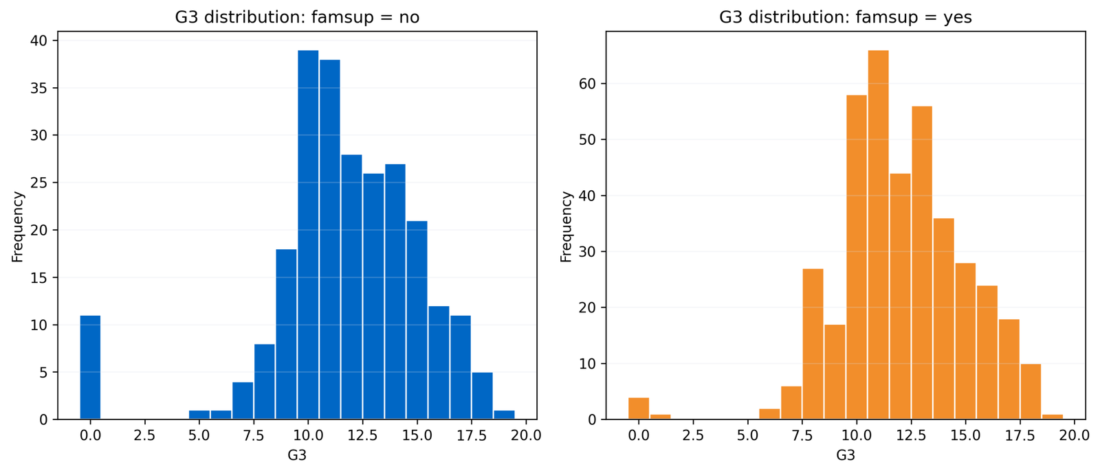
The no-support group peaks at G3 = 10–11 and contains 11 zeros; the support group peaks at G3 = 10–13 and contains 4 zeros.
Both distributions have similar central concentration, but the unsupported group has a visibly heavier lower extreme.
Boxplot by Family Educational Support
Python
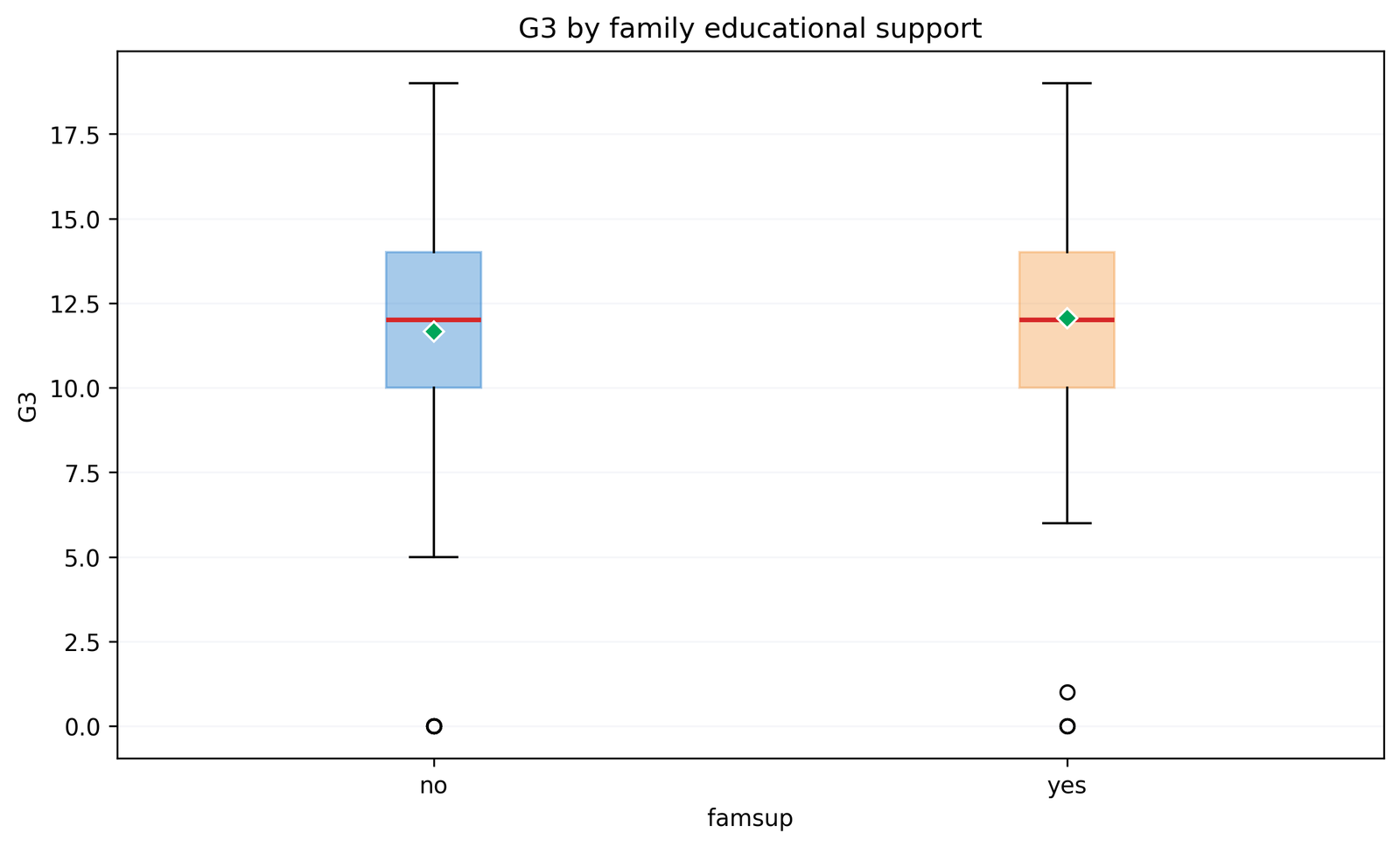
Both boxes extend from Q1 = 10 to Q3 = 14 with median = 12. The no group shows zero-grade outliers; the yes group shows zero and one-grade outliers.
The central 50% is identical, while the lower extremes account for much of the SD difference.
Empirical Cumulative Distributions
Python
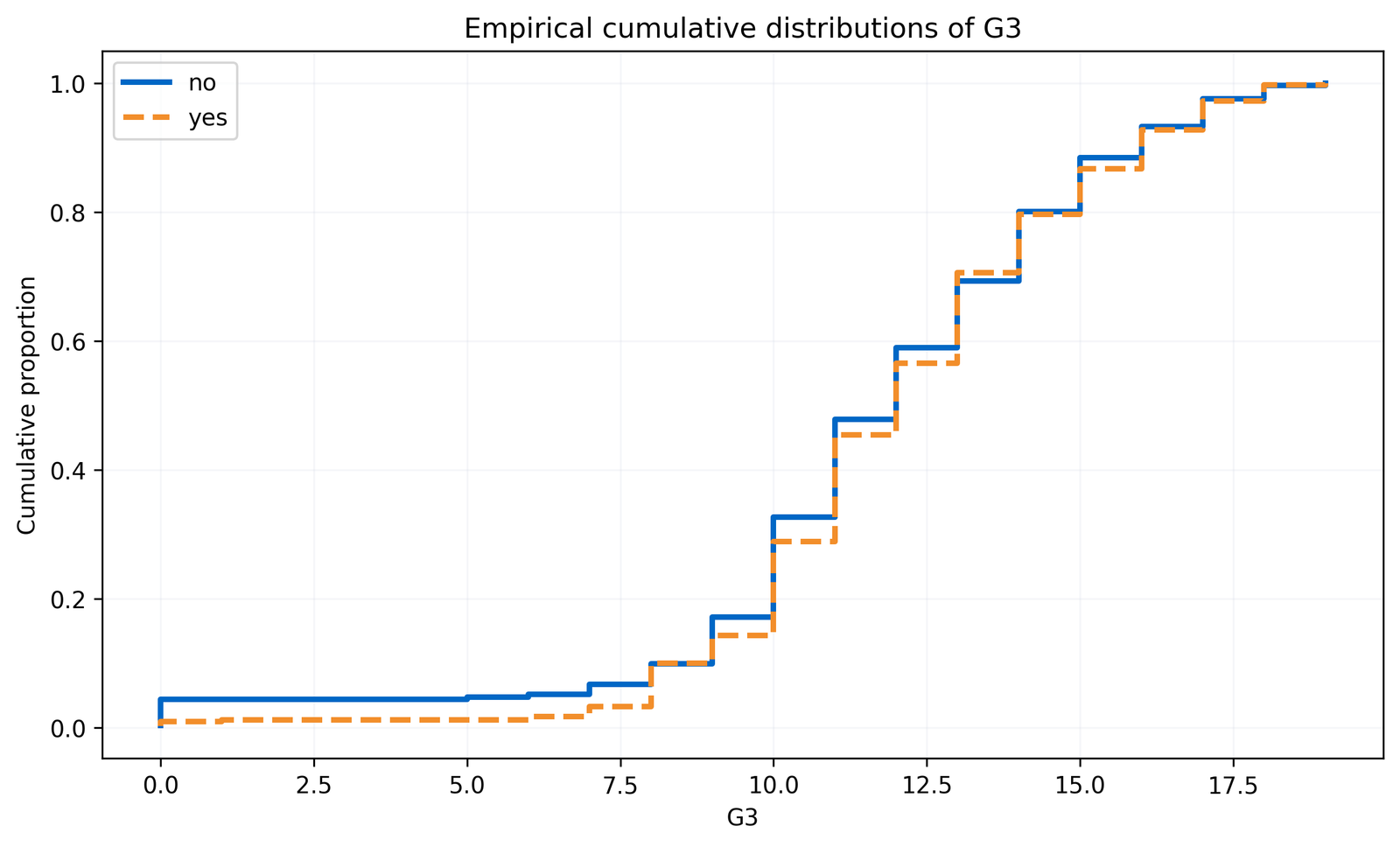
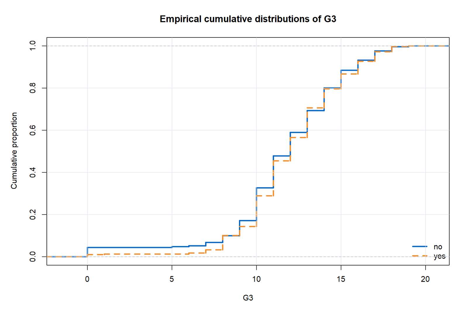
The curves are close through most of the grade range. The largest visible separation is in the low-grade region where the no-support cumulative proportion rises earlier.
Close ECDFs support the conclusion that there is no broad, dramatic scale separation.
Descriptive Dispersion Comparison
Python
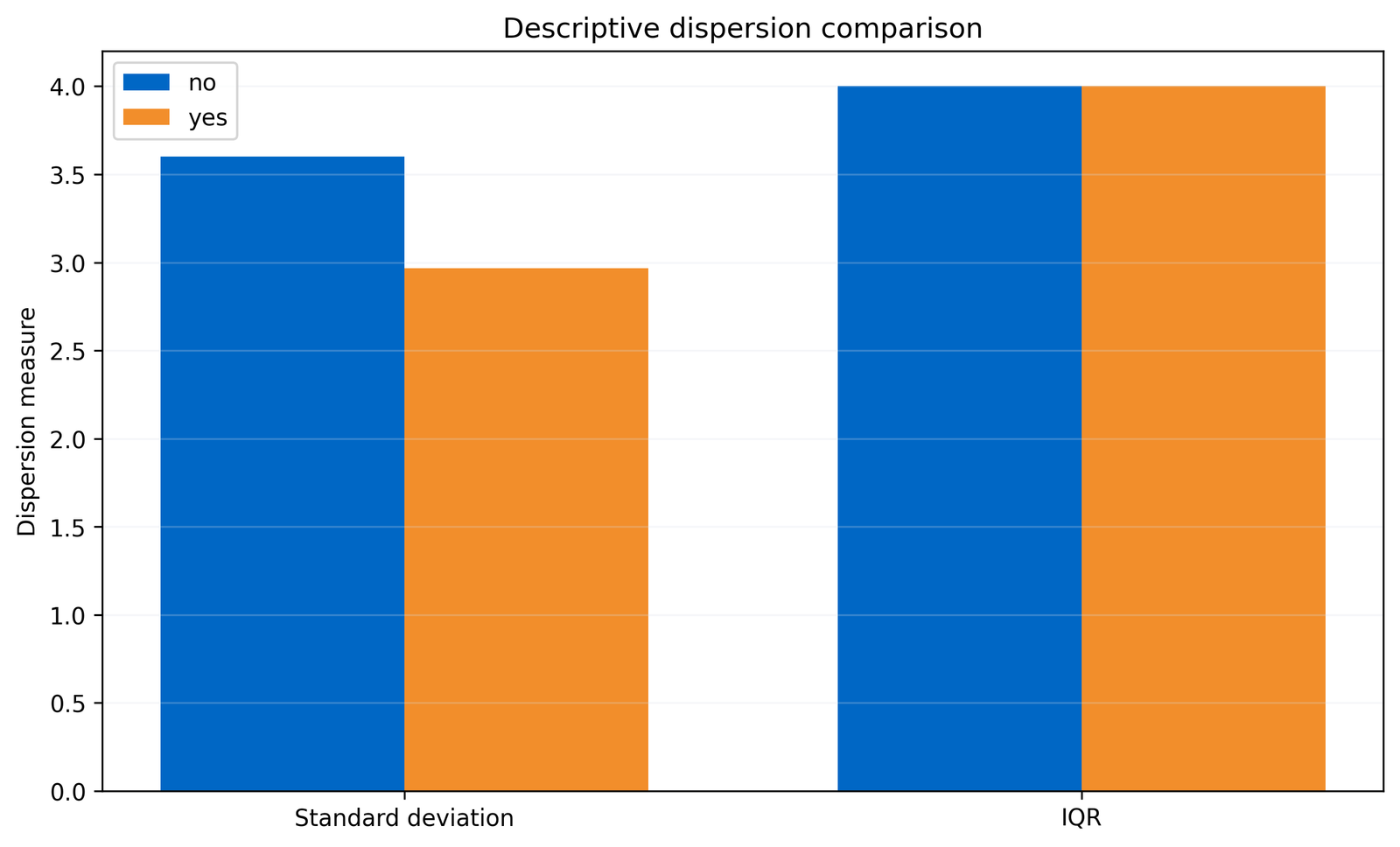
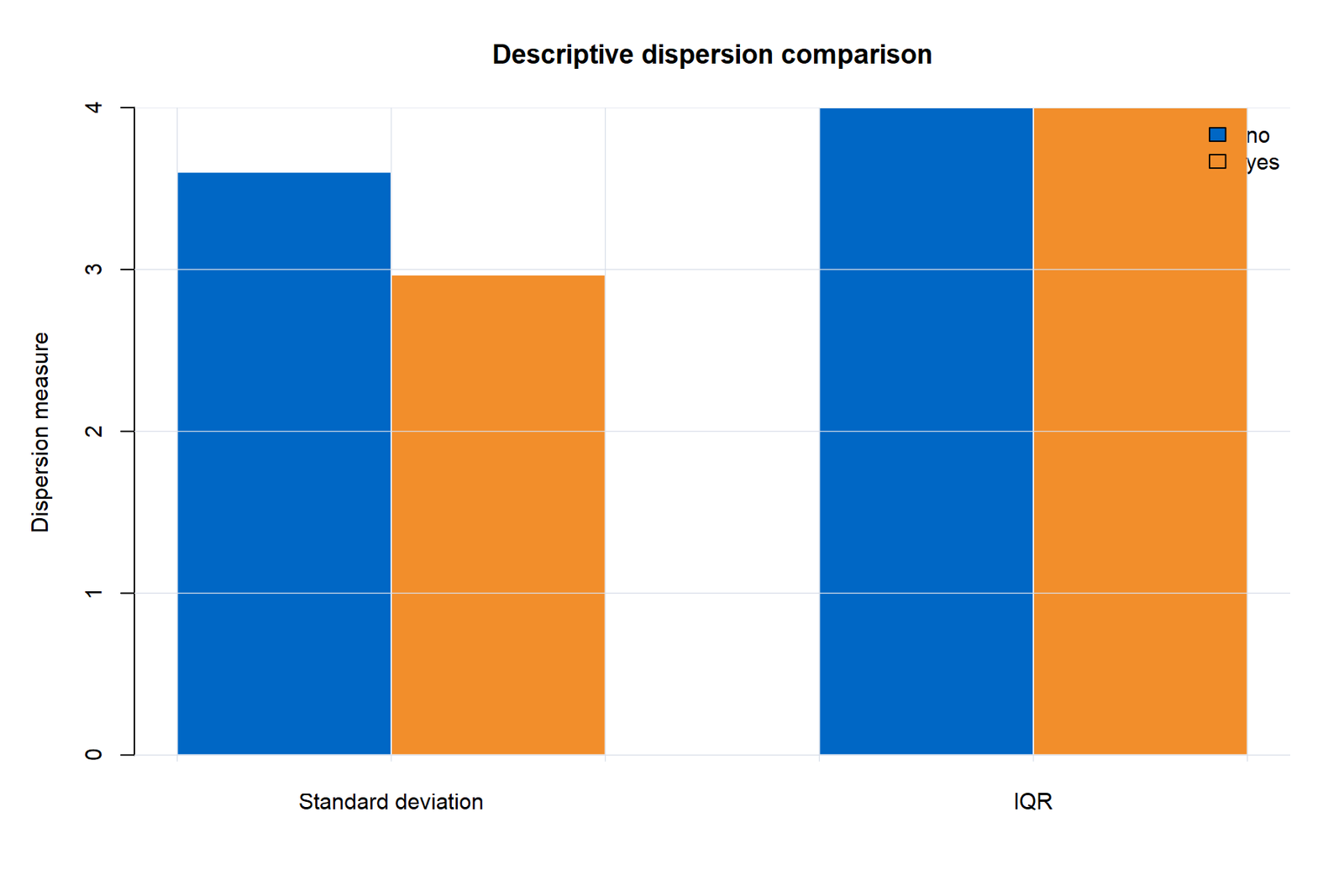
SD is 3.6022 versus 2.9674, while both IQRs equal 4.
The split between SD and IQR tells an important story: tail observations differ more than the central half.
Average Symmetric Score by G3
Python
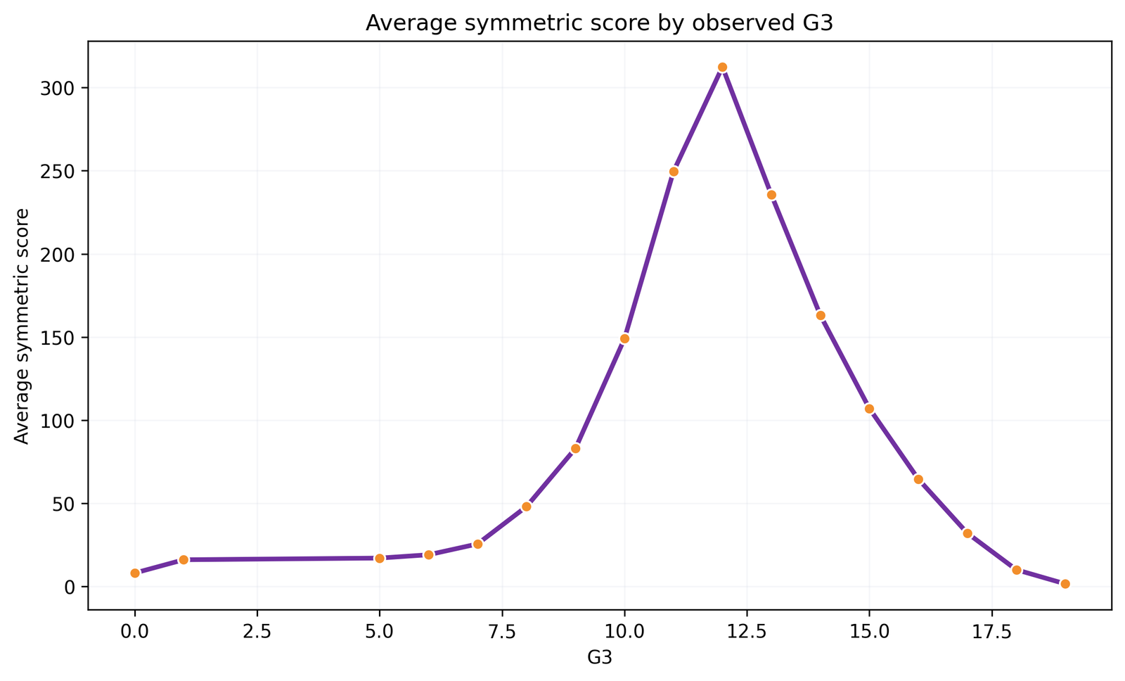
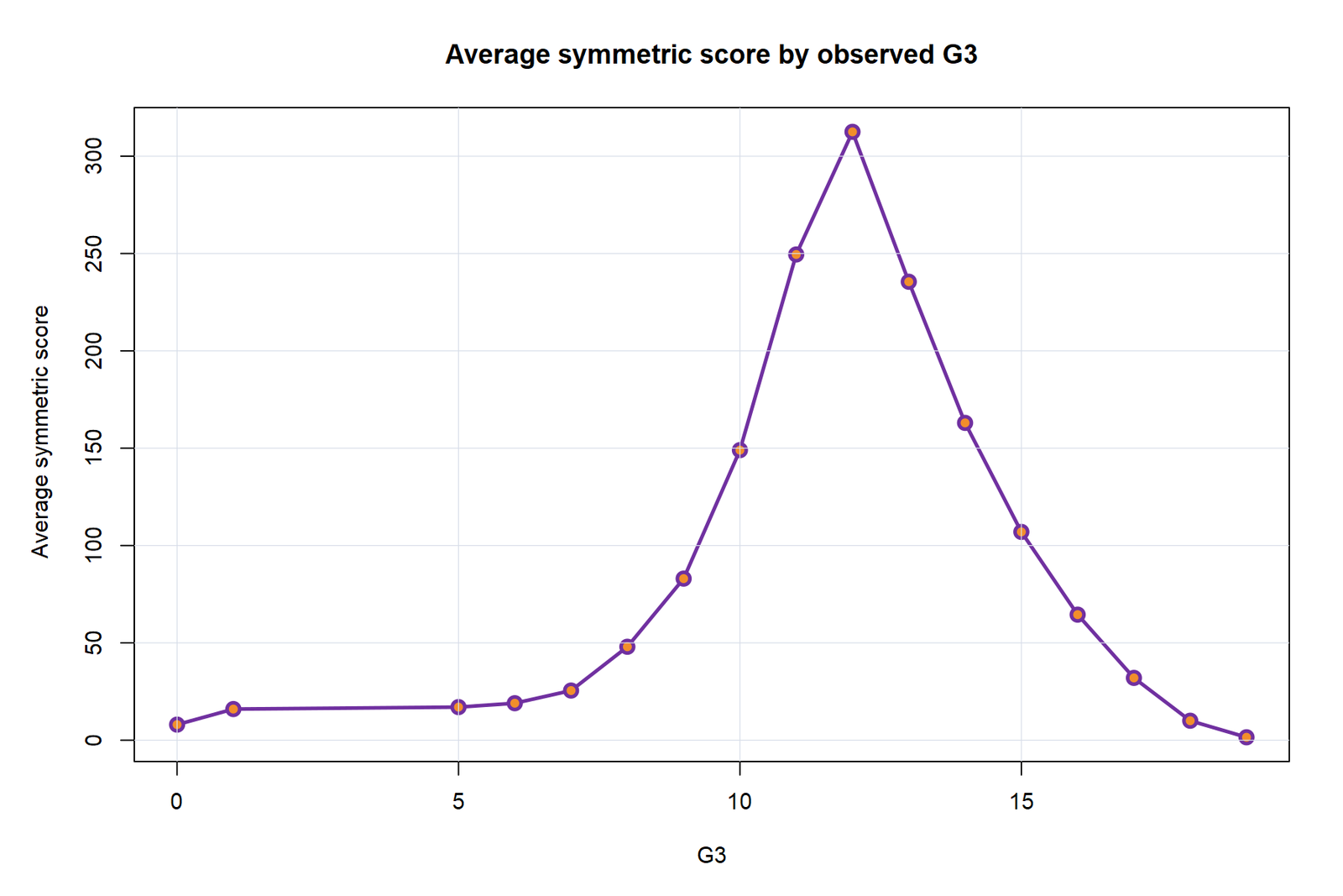
Scores rise from the extremes toward the pooled centre and peak around G3 = 12, then decline toward the upper extreme.
This shape explains the test: central grades contribute large scores, while very low and very high grades contribute small scores.
Deterministic Permutation Distribution
Python
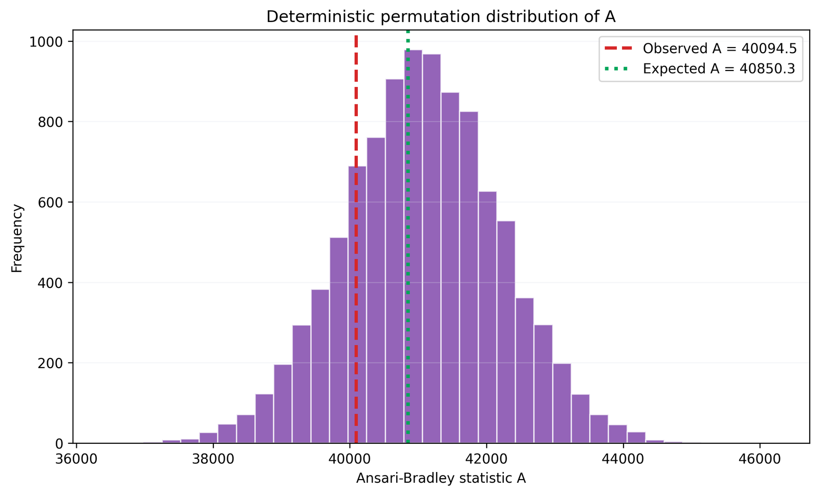
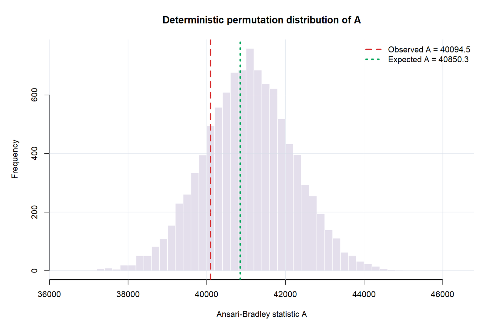
The observed A = 40,094.5 lies left of E(A) = 40,850.3, but remains well inside the main permutation mass. The two-sided permutation p-value is 0.510849.
The observed direction is compatible with somewhat greater no-group dispersion, but the distance from the null centre is not exceptional.
R Verification Gallery: Paired Charts and Independent Checks
The R section is arranged in paired horizontal rows on desktop and collapses cleanly on mobile. It verifies reproducibility without repeating the Python prose word for word.
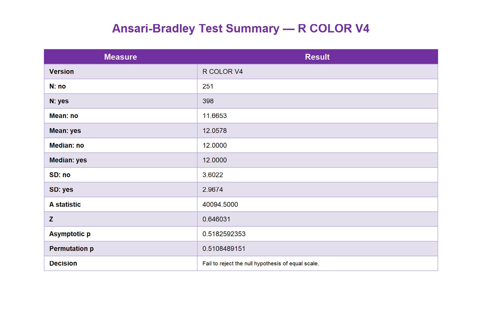
R evidence pair 1
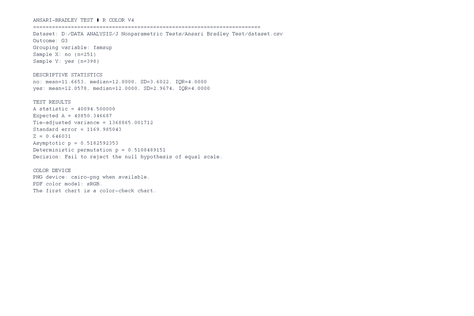
Output report
The R transcript reproduces the group sizes, descriptives, A statistic and two p-values. It serves as an independent implementation check rather than a second substantive analysis.
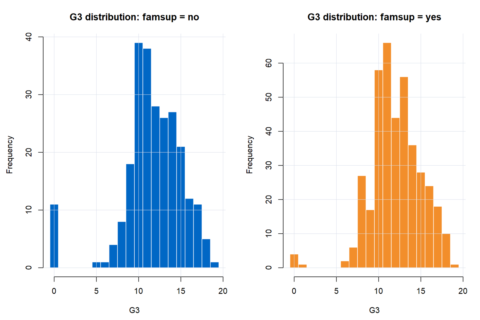
Distribution profile
The R histograms should reproduce the same 0–19 frequency structure as Python. Unequal sample sizes make shape and proportions more informative than absolute heights.
R evidence pair 2
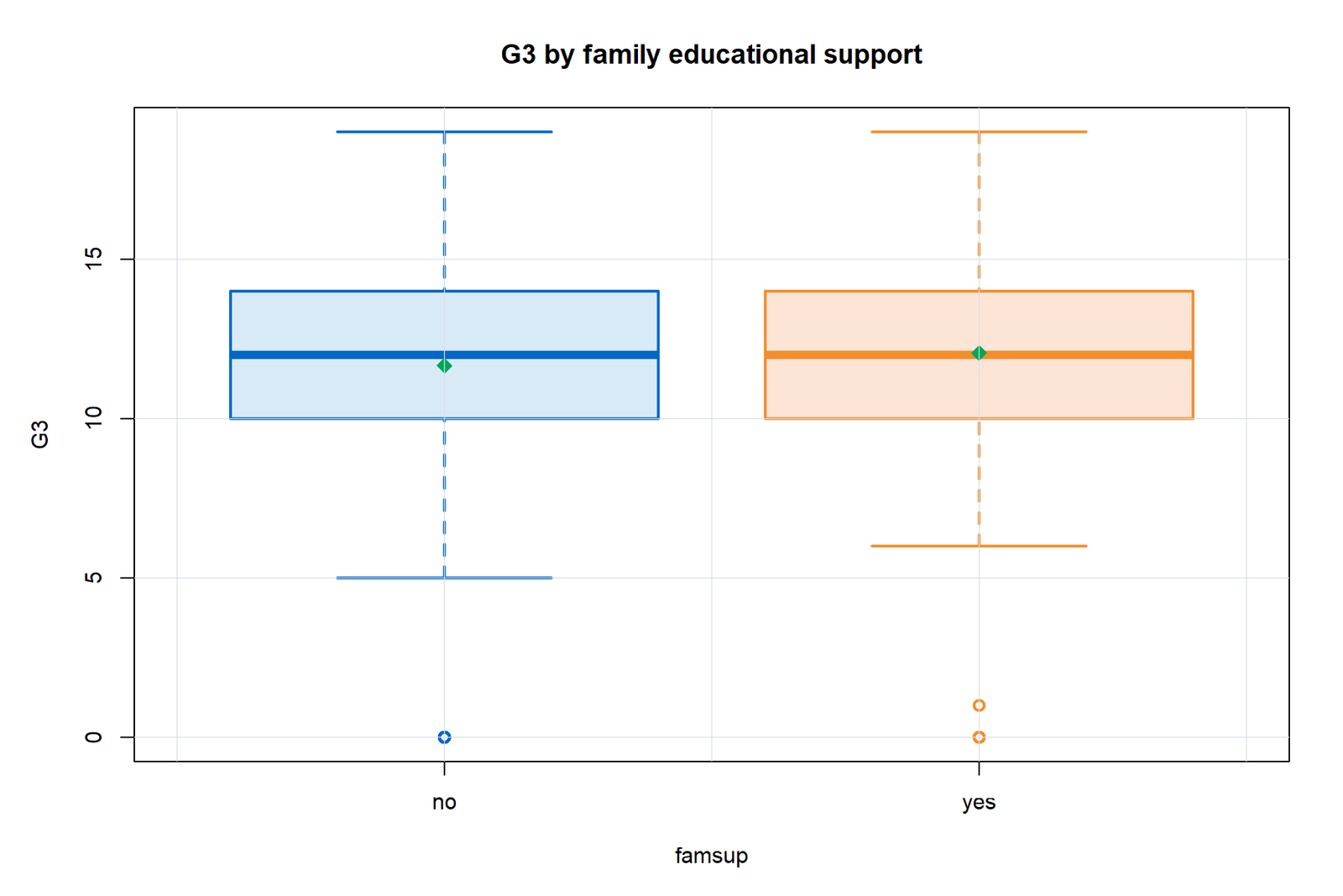
Central spread
The boxplot confirms median 12 and IQR 4 in both groups, with the descriptive difference concentrated outside the boxes.
Cumulative pattern
The R ECDF reproduces the close cumulative trajectories and the low-grade separation visible in Python.
R evidence pair 3
SD versus IQR
The R panel highlights the same contrast: unequal SDs but identical IQRs. This prevents a simplistic claim that every aspect of spread differs.
Score mechanics
The central grades receive high scores and pooled extremes receive low scores. This is the mechanism that turns the raw distributions into A.
R evidence pair 4
Permutation evidence
The R permutation plot places the observed statistic within the central null mass, consistent with p = .510849.
Final result summary
The final R summary consolidates the evidence and should not introduce a competing result or alternative grouping variable.
Python, R, SPSS, SAS and Excel Workflows
Python
- Use
scipy.stats.ansariwith a two-sided alternative. - For this tied large sample, request the asymptotic method or a configured permutation method.
- Recreate frequency, ECDF, score and permutation visuals.
R
- Use
ansari.test(G3 ~ famsup, data = dat, exact = FALSE). - Request a scale-ratio estimate only when its assumptions and tie method are clearly explained.
- Keep the group order fixed so the direction remains interpretable.
SPSS
- Use native SPSS output for descriptives, histograms and boxplots.
- The supplied corrected report includes the separately validated Ansari–Bradley calculation.
- Do not imply that an ordinary
EXAMINEcommand alone produces A.
SAS
- Use
PROC NPAR1WAY ABfor Ansari–Bradley scores. - The
EXACT AB / MCworkflow can estimate an exact-reference p-value by Monte Carlo for large problems. - Preserve the two-level class variable and numeric response.
Excel
- Pool and rank G3 with
RANK.AVG. - Convert each pooled rank to a symmetric score.
- Sum sample-X contributions and calculate expectation, tie-adjusted variance, z and p.
Cross-Software Rule
- Group order, tie handling and p-value method must be documented.
- Two-sided p-values should agree to displayed precision.
- A reversed z sign is acceptable only when the direction convention is stated.
Expandable Reproducible Code
Python: SciPy asymptotic and permutation workflows
from scipy import stats
from scipy.stats import PermutationMethod

x = df.loc[df["famsup"].eq("no"), "G3"].dropna().to_numpy()
y = df.loc[df["famsup"].eq("yes"), "G3"].dropna().to_numpy()

asym = stats.ansari(x, y, alternative="two-sided", method="asymptotic")
perm = stats.ansari(
    x, y,
    alternative="two-sided",
    method=PermutationMethod(n_resamples=10_000, random_state=12345)
)

print(asym.statistic, asym.pvalue)
print(perm.statistic, perm.pvalue)
R: ansari.test and descriptive audit
dat$famsup <- factor(dat$famsup, levels = c("no", "yes"))
fit <- ansari.test(
  G3 ~ famsup,
  data = dat,
  alternative = "two.sided",
  exact = FALSE
)
print(fit)

# Descriptive audit
aggregate(G3 ~ famsup, dat, function(x)
  c(n = length(x), mean = mean(x), median = median(x),
    sd = sd(x), variance = var(x), IQR = IQR(x)))
SPSS: native descriptives and corrected integrated result
* Native descriptive and visual audit.
EXAMINE VARIABLES=G3 BY famsup
 /PLOT=BOXPLOT HISTOGRAM
 /COMPARE=GROUP
 /STATISTICS=DESCRIPTIVES
 /CINTERVAL=95
 /MISSING=LISTWISE.

* The supplied corrected report then integrates the
* separately validated Ansari-Bradley A, tie-adjusted
* variance, z, asymptotic p, and permutation p.
SAS: PROC NPAR1WAY with Ansari–Bradley scores
proc npar1way data=student_data ab;
  class famsup;
  var G3;
  exact ab / mc n=10000 seed=12345;
run;
Excel: key workbook formulas
Pooled rank:
=RANK.AVG(C4,$C$4:$C$652,1)

Symmetric score:
=MIN(D4,COUNT($C$4:$C$652)-D4+1)

Sample-X contribution:
=IF(B4=Results!$B$7,E4,0)

Observed A:
=SUM(AB_Calculation!$F$4:$F$652)

Expected A for odd N:
=nX*(N+1)^2/(4*N)

Two-sided p:
=2*(1-NORM.S.DIST(ABS(z),TRUE))
Cross-Software Reconciliation
| Output | Python | R | SPSS corrected report | Excel V4 | Status |
|---|---|---|---|---|---|
| Sample sizes | 251 / 398 | 251 / 398 | 251 / 398 | 251 / 398 | Match |
| Medians | 12 / 12 | 12 / 12 | 12 / 12 | 12 / 12 | Match |
| Standard deviations | 3.6022 / 2.9674 | 3.6022 / 2.9674 | 3.602 / 2.967 | 3.6022 / 2.9674 | Match |
| A statistic | 40,094.5 | 40,094.5 | 40,094.5 | 40,094.5 | Match |
| Z statistic | 0.646031 or sign-reversed by convention | 0.646031 or sign-reversed by convention | 0.646031 | 0.646031 | Magnitude matches |
| Asymptotic p | 0.518259 | 0.518259 | 0.518259 | 0.518259 | Match |
| Permutation p | 0.510849 | 0.510849 | 0.510849 | 0.510849 | Match |
Ansari–Bradley Test Compared with Related Methods
| Method | Primary target | Groups | Distribution requirement | Important distinction |
|---|---|---|---|---|
| Ansari–Bradley | Scale parameter | 2 | Common location; rank-score model | Current method; symmetric extreme-to-centre scores. |
| Mood scale test | Scale parameter | 2 | Rank-based | Alternative two-sample scale score system. |
| Siegel–Tukey | Scale parameter | 2 | Rank-based; common location | Alternating extreme-rank scoring. |
| Fligner–Killeen | Homogeneity of spread | 2 or more | Robust and rank-based | Natural extension for multiple groups. |
| Levene test | Variance homogeneity | 2 or more | Reasonably robust, depending on centre choice | Uses absolute deviations from a group centre. |
| Brown–Forsythe | Variance homogeneity | 2 or more | Robust median-centred version of Levene | Useful when skewness and outliers are present. |
| Bartlett test | Variance homogeneity | 2 or more | Sensitive to non-normality | Powerful under normality but fragile otherwise. |
| Two-sample F test | Variance ratio | 2 | Normal populations | Direct parametric variance-ratio test. |
| Mann–Whitney U | Location / stochastic ordering | 2 | Independent groups | Not a substitute for a scale question. |
| Brunner–Munzel | Relative stochastic effect | 2 | Allows unequal variances | Targets ordering, not scale equality. |
| Lepage test | Joint location and scale | 2 | Rank-based combined framework | Useful when both components are scientifically relevant. |
APA-Style Reporting and Research Write-Up
Concise Result
An Ansari–Bradley test found no statistically significant difference in G3 scale between students without family educational support (n = 251) and students with support (n = 398), A = 40,094.50, z = 0.65, p = .518.
Full Result with Verification
An Ansari–Bradley test was used to compare the dispersion of G3 scores between students without family educational support (n = 251) and those with support (n = 398). Both groups had a median of 12 and an interquartile range of 4. The scale difference was not statistically significant, A = 40,094.50, z = 0.65, p = .518. A deterministic 10,000-permutation analysis produced a consistent result, p = .511. Although the no-support group had a larger sample standard deviation, 3.60 versus 2.97, the analysis did not provide sufficient evidence of different population scale.
Reusable Reporting Template
An Ansari–Bradley test compared the scale of outcome between group X and group Y.
The group medians were median X and median Y, supporting / questioning the common-location condition.
The result was A = value, z = value, p = value.
A permutation or exact-reference analysis gave p = value.
The analysis did / did not provide evidence of a population-scale difference.
Common Ansari–Bradley Test Mistakes
The procedure targets scale under a common-location model.
Location differences can contaminate the scale interpretation.
A nonsignificant test does not prove equality.
Large tied samples require an appropriate asymptotic or permutation method.
Descriptive ratios do not supply a p-value.
A scale ratio s corresponds to a variance ratio s² when variances exist.
Brunner–Munzel gender charts do not belong in this family-support scale analysis.
The A statistic and directional interpretation depend on the focal sample.
Select a k-sample scale procedure instead.
Practice Questions with Answers
Question 1: What parameter does the Ansari–Bradley test target?
Answer: The relative scale or dispersion of two independent populations under a common-location model.
Question 2: Why is the equal-median check important?
Answer: A material location shift can change which observations appear central or extreme, weakening a pure scale interpretation.
Question 3: Both groups have IQR = 4, but their SDs differ. Is this contradictory?
Answer: No. IQR describes the middle 50%, whereas SD is sensitive to tail observations such as zero grades.
Question 4: What does A = 40,094.5 represent?
Answer: It is the sum of the symmetric pooled scores for the focal no-support group.
Question 5: What is the null expectation of A in this analysis?
Answer: 40,850.3467.
Question 6: Why can different software report z with opposite signs?
Answer: One implementation may standardize A − E(A), while another uses E(A) − A. The two-sided p-value is unchanged.
Question 7: Why is the permutation p-value useful here?
Answer: It verifies the decision without relying only on the large-sample normal reference in a heavily tied dataset.
Question 8: Can p = .518 prove equal dispersion?
Answer: No. It indicates insufficient evidence to reject equal scale; it is not an equivalence result.
Question 9: Which group is descriptively more variable?
Answer: The no-support group, with SD 3.6022 versus 2.9674 and variance ratio 1.4736.
Question 10: Where is the descriptive difference concentrated?
Answer: Mainly in the lower tail, especially the higher proportion of G3 = 0 in the no-support group.
Question 11: Which test is a better starting point for three groups?
Answer: Fligner–Killeen or another justified k-sample spread test.
Question 12: Should the Z Test for Proportions be linked as a primary related method?
Answer: No. It addresses binary proportions, not a two-sample scale parameter.
Verified Ansari–Bradley Downloads
R Color V4 ReportIndependent R verification and colour chart output.
Corrected SPSS ReportSPSS descriptives, charts and integrated validated test result.
Worked Excel V4Raw data, pooled ranks, symmetric scores, formulas and results.
Frequently Asked Questions
What is the Ansari–Bradley test?
It is a nonparametric two-sample test for a difference in scale parameters. It uses symmetric scores assigned to pooled ranks from the extremes toward the centre.
Is the Ansari–Bradley test a test of equal medians?
No. Equal or aligned location is a condition supporting the scale interpretation; the statistic itself targets dispersion.
What does a smaller A statistic mean?
For the focal sample, a smaller-than-expected A generally indicates more observations at the pooled extremes and therefore a direction consistent with larger scale.
Why are ties important in this dataset?
G3 is an integer grade, so many students share the same value. Midranks and a tie-adjusted variance are required, and a permutation check strengthens the inference.
What is the result for family educational support?
A = 40,094.5, z = 0.6460, asymptotic p = .5183 and permutation p = .5108. The equal-scale null is not rejected.
Why is the no-support standard deviation larger?
That group contains a higher proportion of very low scores, especially zeros, which increase squared deviations from the mean.
Can I conclude the populations have the same variance?
No. A nonsignificant result means the data do not provide sufficient evidence of a scale difference. Formal equivalence requires a separate design and margin.
What is the difference between a scale ratio and a variance ratio?
When variances exist, a scale ratio s corresponds to a variance ratio s squared. They should not be reported as though they are the same quantity.
Can the test be used with more than two groups?
The classic Ansari–Bradley test is a two-sample procedure. A k-sample method such as Fligner–Killeen is more appropriate for multiple groups.
What should be reported?
Report group sizes, medians or location audit, A, the inference method, p-value, decision and a careful scale-focused interpretation.
Conclusion
The Ansari–Bradley test provides a focused nonparametric comparison of scale for two independent populations. In the worked G3 analysis, the data satisfy the most important descriptive location check: both family-support groups have a median of 12 and an IQR of 4. The group without support nevertheless has a larger sample SD and variance, driven primarily by a heavier lower tail.
The formal rank-score evidence does not confirm a population-scale difference. The observed A statistic of 40,094.5 is only 0.646 standard errors from its equal-scale expectation. The tie-adjusted asymptotic p-value of .5183 and deterministic permutation p-value of .5108 agree closely. The correct conclusion is therefore that no statistically significant difference in G3 scale was detected—not that the two populations have been proven identical.