
Nominal association, chi-square test, contingency table and effect size
Cramer’s V: Formula, Interpretation, Python, R, SPSS and Excel Guide
Cramer’s V is an effect size measure for association between two categorical variables. It is commonly reported after a chi-square test of independence because the chi-square p-value tells whether an association is statistically detectable, while Cramer’s V tells how strong the association is. This guide explains Cramer’s V with Python charts, R charts, SPSS output, Excel formulas, observed counts, expected counts, row percentages, residuals, chi-square contributions and APA reporting.
Quick Answer: Cramer’s V Result
The worked example tests the association between school and sex. The row variable is school, with categories GP and MS. The column variable is sex, with categories F and M. The sample size is N = 649.
The chi-square test gives χ²(1) = 4.4763 with p = 0.03437. Cramer’s V is 0.08305, and the bias-corrected Cramer’s V is 0.07323. The association is statistically significant at α = .05, but the effect size is very weak / negligible.
Final interpretation: School and sex show a statistically significant association, but the size of that association is very small. The practical difference between schools is weak even though the p-value is below .05.
Important reporting rule: Do not report only the chi-square p-value. A large dataset can produce a significant p-value for a weak pattern. Report both χ² and Cramer’s V so the reader sees both statistical evidence and practical strength.
Table of Contents
- What Is Cramer’s V?
- Cramer’s V Formula
- Dataset and Variables Used
- Verified Cramer’s V Results
- Python Chart-by-Chart Interpretation
- R Chart-by-Chart Interpretation
- SPSS Output Interpretation
- Excel Worked File Explanation
- Python, R, SPSS and Excel Workflows
- Code Blocks and Excel Formulas
- How to Report Cramer’s V
- Common Mistakes
- Downloads and Resources
- Related Statistical Guides
- FAQs About Cramer’s V
What Is Cramer’s V?
Cramer’s V measures the strength of association between two categorical variables. It is based on the chi-square statistic and ranges from 0 to 1. A value near 0 means little or no association. A value closer to 1 means a stronger association.
Cramer’s V is especially useful for nominal variables because ordinary Pearson correlation is not appropriate for unordered categories such as school, sex, address type, treatment group or response category. The chi-square test asks whether the variables are independent. Cramer’s V explains how large the association is after the independence test.
This makes Cramer’s V closely connected with cross tabulation, p-value, effect size, frequency distribution, null and alternative hypothesis and statistical power.
Simple definition: Cramer’s V is the effect size for a chi-square association between categorical variables.
Cramer’s V Formula
The standard Cramer’s V formula is:
In this formula, χ² is the Pearson chi-square statistic, N is the total sample size, r is the number of row categories and c is the number of column categories. The term min(r − 1, c − 1) adjusts the effect size for the smaller dimension of the contingency table.
| Symbol | Meaning | Value in This Example |
|---|---|---|
| χ² | Pearson chi-square statistic | 4.476302 |
| N | Total valid sample size | 649 |
| r | Number of row categories | 2 |
| c | Number of column categories | 2 |
| min(r − 1, c − 1) | Minimum table dimension adjustment | 1 |
| V | Cramer’s V | 0.083050 |
The chi-square statistic itself is calculated from observed and expected counts:
Expected counts are calculated as:
Dataset and Variables Used
The example uses two categorical variables from the student performance dataset. The row variable is school, and the column variable is sex.
| Variable | Role | Categories | Purpose |
|---|---|---|---|
| school | Row variable | GP, MS | Compares two schools. |
| sex | Column variable | F, M | Compares student sex categories. |
| Observed counts | Input table | 2 × 2 cells | Used to calculate expected counts and chi-square. |
| Cramer’s V | Effect size | 0 to 1 | Measures strength of association. |
The observed contingency table is:
| School | F | M | Row Total |
|---|---|---|---|
| GP | 237 | 186 | 423 |
| MS | 146 | 80 | 226 |
| Total | 383 | 266 | 649 |
Verified Cramer’s V Results
The Python, R, SPSS and Excel outputs use the same contingency table for school by sex. The final test is statistically significant, but the association strength is very weak.
| Result Item | Value | Interpretation |
|---|---|---|
| Sample size | 649 | All students were valid for school and sex. |
| Rows | 2 | Two school categories: GP and MS. |
| Columns | 2 | Two sex categories: F and M. |
| Pearson chi-square | 4.476302 | Difference between observed and expected counts. |
| Degrees of freedom | 1 | (2 − 1) × (2 − 1). |
| p-value | 0.034368 | Statistically significant at α = .05. |
| Cramer’s V | 0.083050 | Very weak / negligible association. |
| Bias-corrected Cramer’s V | 0.073228 | Optional corrected effect size. |
| Decision | Significant association | The pattern is detectable, but small. |
The practical meaning is clear: the proportion of female and male students differs slightly between schools, but the difference is small. The p-value says the variables are not perfectly independent. Cramer’s V says the association strength is weak.
Python Chart-by-Chart Interpretation
The Python charts show the observed table, expected table, row percentage profile, standardized residuals, chi-square cell contribution and final effect size summary.
Python Chart 1: Observed Counts Heatmap
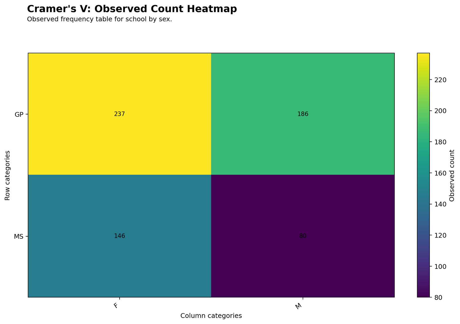
The observed heatmap shows the real cell counts used in the analysis. GP has 237 female and 186 male students, while MS has 146 female and 80 male students. These four cells are the raw inputs for the chi-square test and Cramer’s V.
The heatmap makes the table easier to read than raw numbers alone. GP has more students overall than MS, so its counts are larger. Interpretation should therefore rely on expected counts, percentages and residuals rather than raw counts only.
Python Chart 2: Expected Counts Heatmap
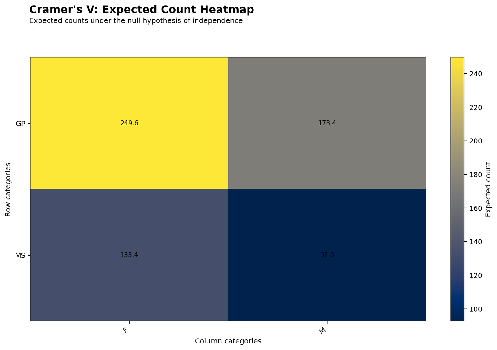
The expected count heatmap shows what the table would look like if school and sex were independent. The expected counts are approximately GP-F = 249.6, GP-M = 173.4, MS-F = 133.4 and MS-M = 92.6.
The observed table differs from this independence pattern. GP has fewer female students than expected and more male students than expected. MS has more female students than expected and fewer male students than expected. These differences create the chi-square statistic.
Python Chart 3: Row Percentage Profile
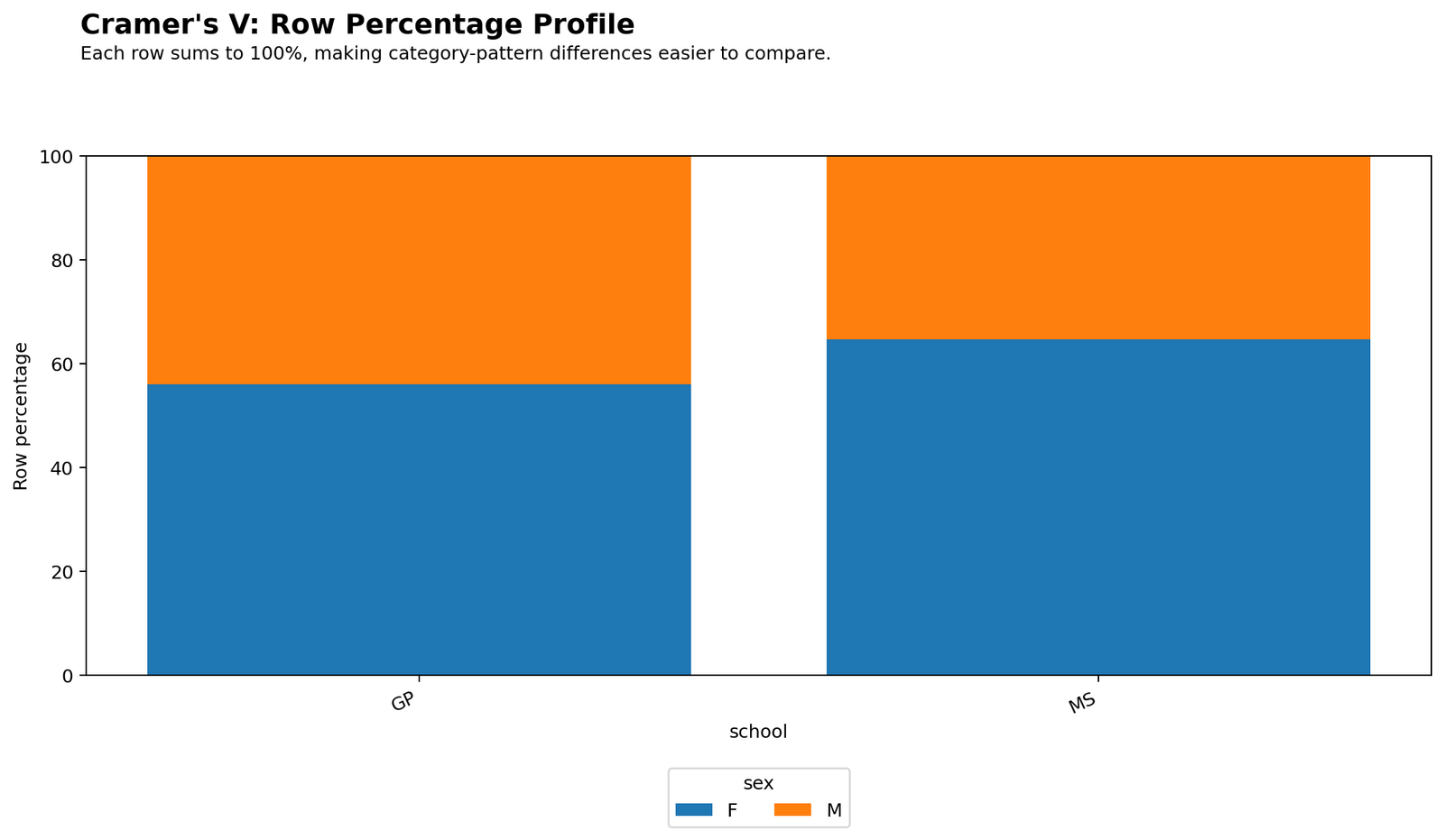
The row percentage profile compares the percentage distribution within each school. GP is about 56.0% female and 44.0% male. MS is about 64.6% female and 35.4% male.
This chart gives the clearest practical interpretation. MS has a higher female percentage than GP, and GP has a higher male percentage than MS. However, the gap is not large, which explains why Cramer’s V is only 0.083.
Python Chart 4: Standardized Residuals Heatmap
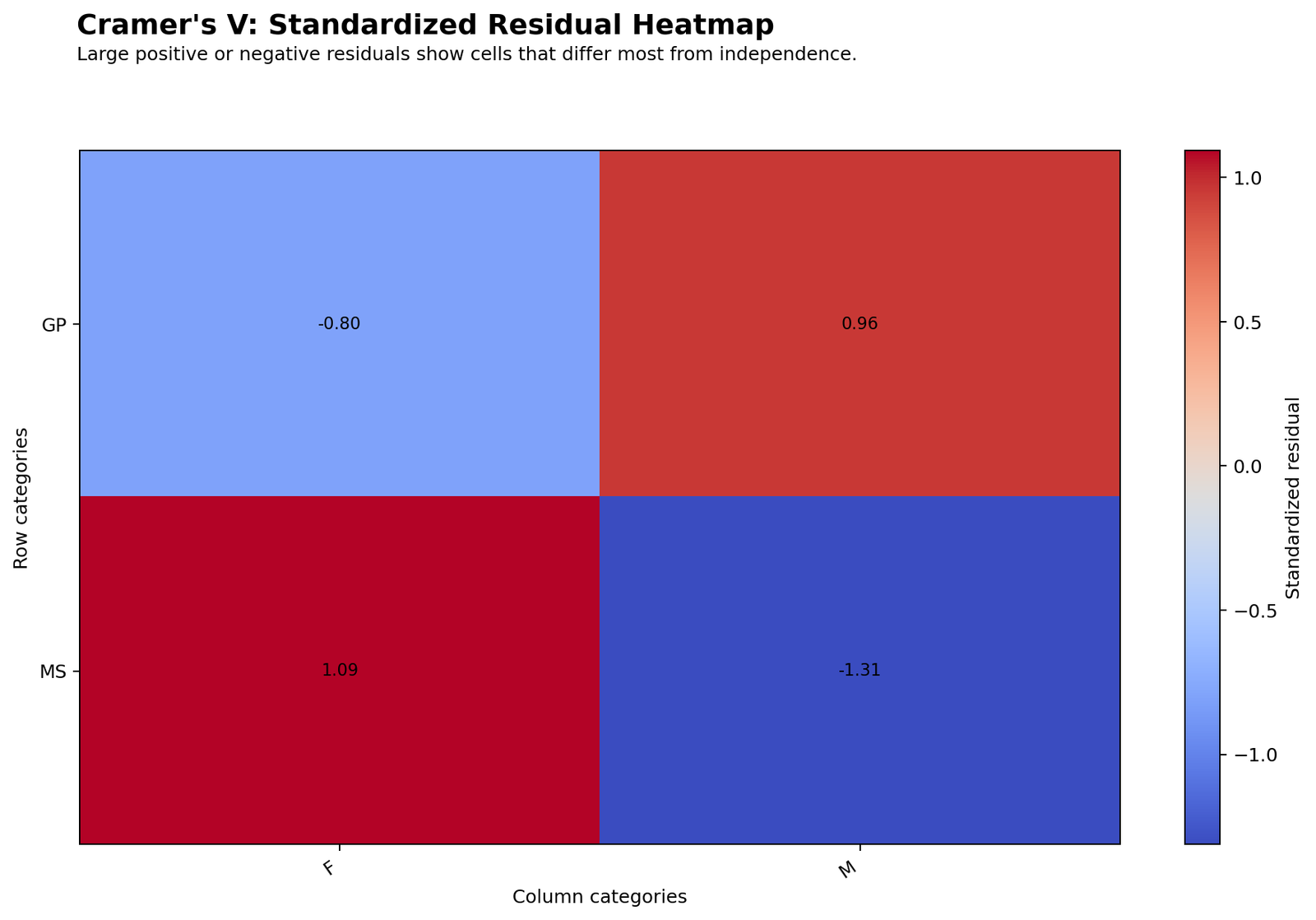
The standardized residuals show which cells are above or below the independence expectation. GP-F is negative, GP-M is positive, MS-F is positive and MS-M is negative. The largest standardized residual in magnitude is around -1.31 for MS-M.
These residuals are not extremely large. That supports the effect size conclusion: the association is statistically detectable, but the practical departure from independence is very small.
Python Chart 5: Chi-Square Cell Contribution
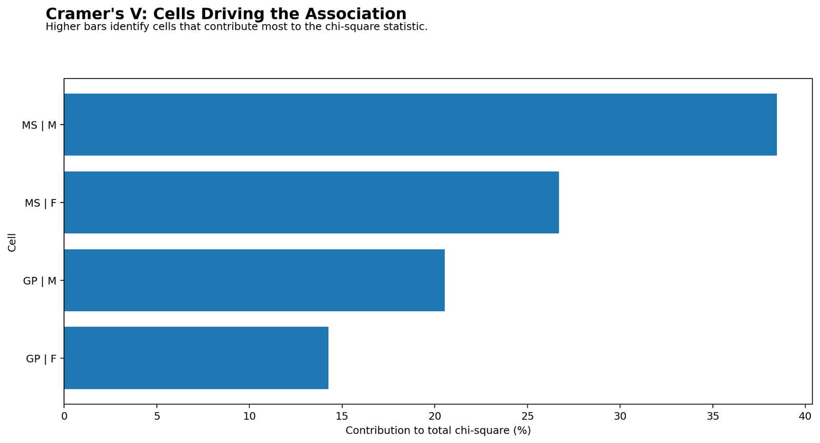
The chi-square contribution chart shows which cells drive the total χ² value. The MS-M and MS-F cells contribute more than the GP cells because their observed counts are farther from expected counts relative to their expected frequencies.
This chart helps explain the test result beyond one p-value. It shows that the association comes from a small but consistent shift in the sex distribution across schools.
Python Chart 6: Effect Size Summary
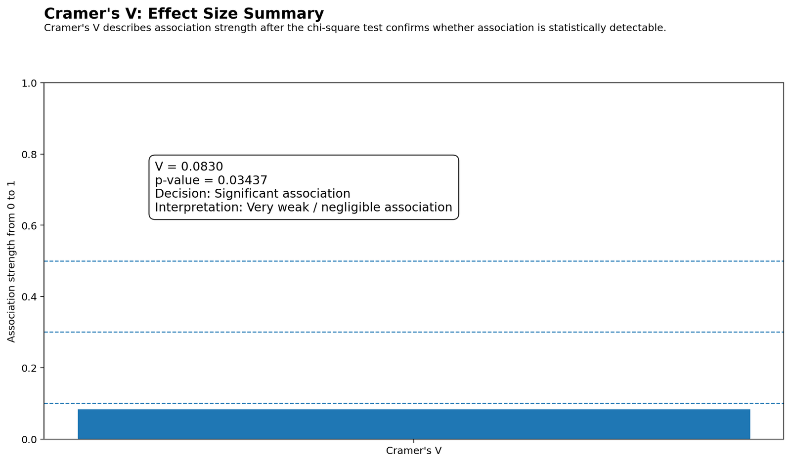
The effect size summary places V = 0.083 on a 0-to-1 scale. It is below the common weak threshold of 0.10, so it is best described as very weak or negligible.
This is the chart to use in the final conclusion. It prevents overstatement: the association is significant, but its strength is small.
R Chart-by-Chart Interpretation
The R charts validate the same Cramer’s V result with colorful output. They repeat the observed counts, expected counts, row percentages, residuals, chi-square contributions and effect size summary.
R Chart 1: Colorful Observed Counts Heatmap
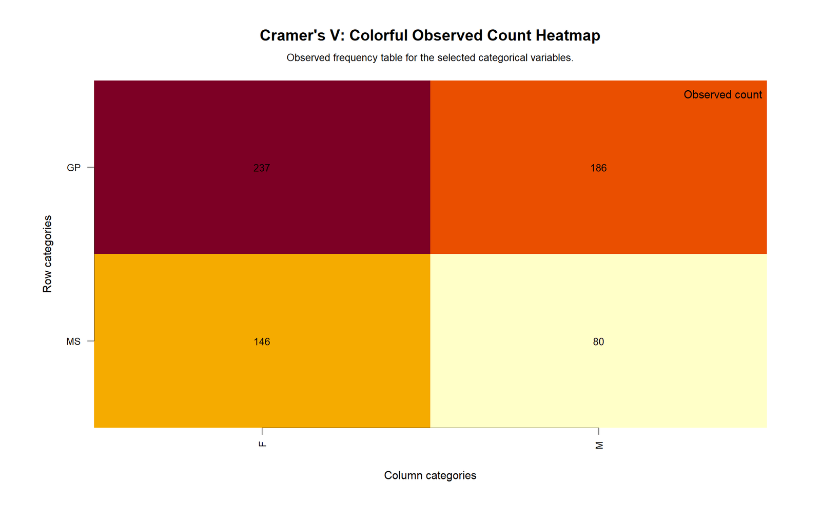
The R observed heatmap confirms the same 2 × 2 table: GP has 237 female and 186 male students, while MS has 146 female and 80 male students. The larger GP counts reflect the larger GP sample size.
R Chart 2: Colorful Expected Counts Heatmap
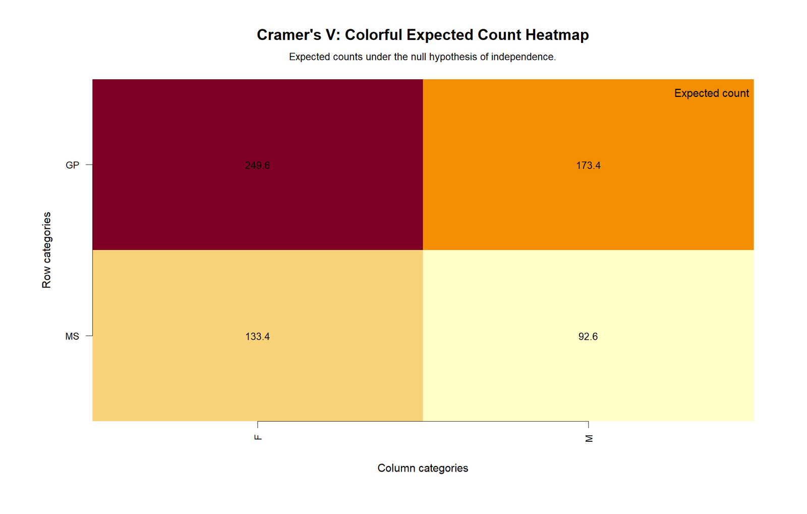
The R expected count heatmap shows the independence baseline. GP-F is expected to be about 249.6, but observed is 237. MS-M is expected to be about 92.6, but observed is 80. These differences produce the chi-square result.
R Chart 3: Colorful Row Percentage Profile
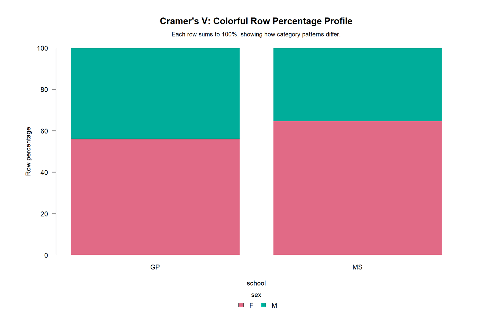
The row percentage chart shows that MS has a higher female percentage than GP. GP is about 56.0% female and 44.0% male; MS is about 64.6% female and 35.4% male. This difference is visible but not large.
R Chart 4: Colorful Standardized Residuals Heatmap
The residual heatmap confirms that the largest cell departures are still modest. No cell shows a very extreme standardized residual. That is why the final Cramer’s V remains very small.
R Chart 5: Colorful Chi-Square Contribution
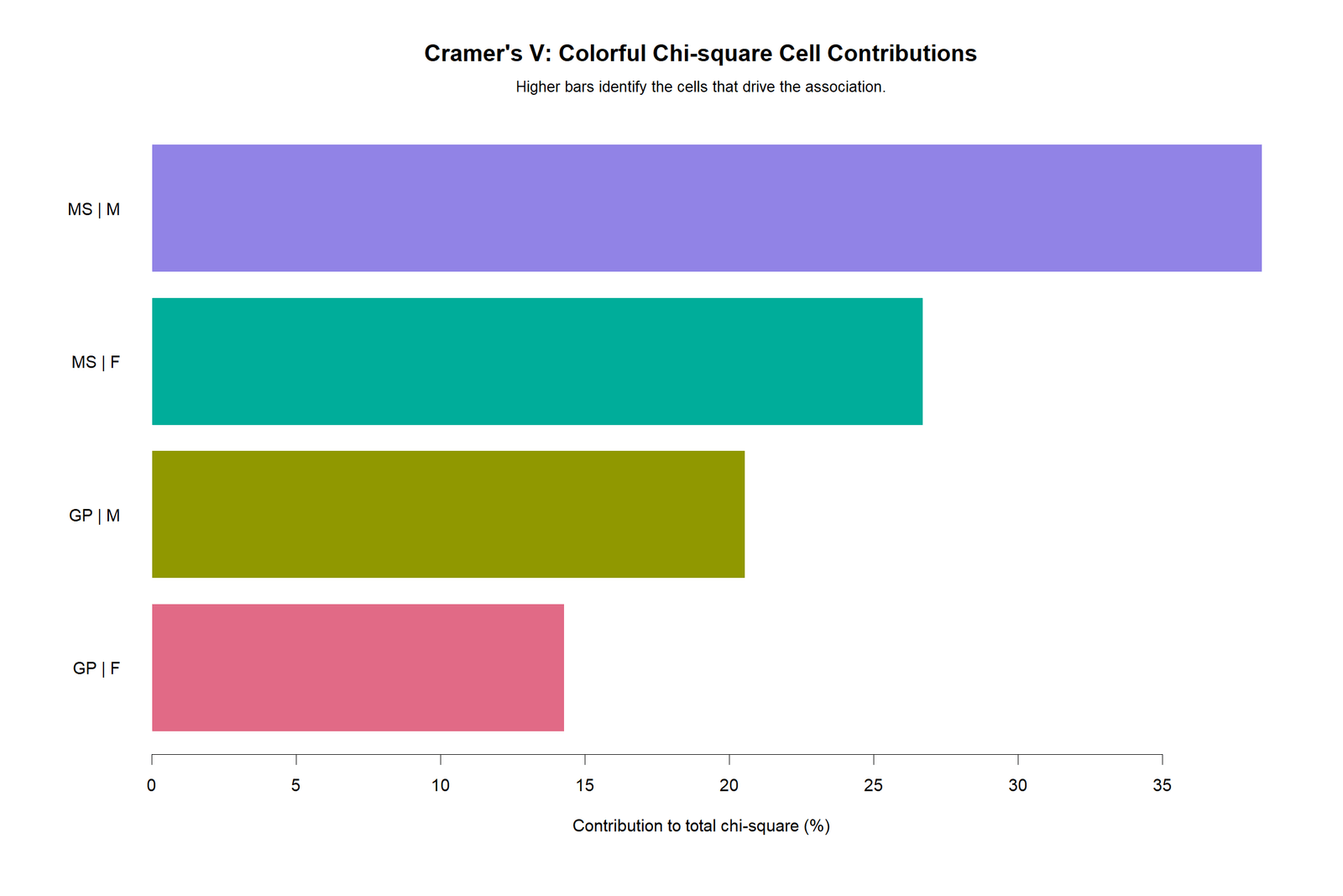
The R contribution chart identifies the cells most responsible for the chi-square statistic. MS-M and MS-F provide relatively larger contributions than the GP cells, but the overall total is still modest at χ² = 4.4763.
R Chart 6: Colorful Effect Size Summary
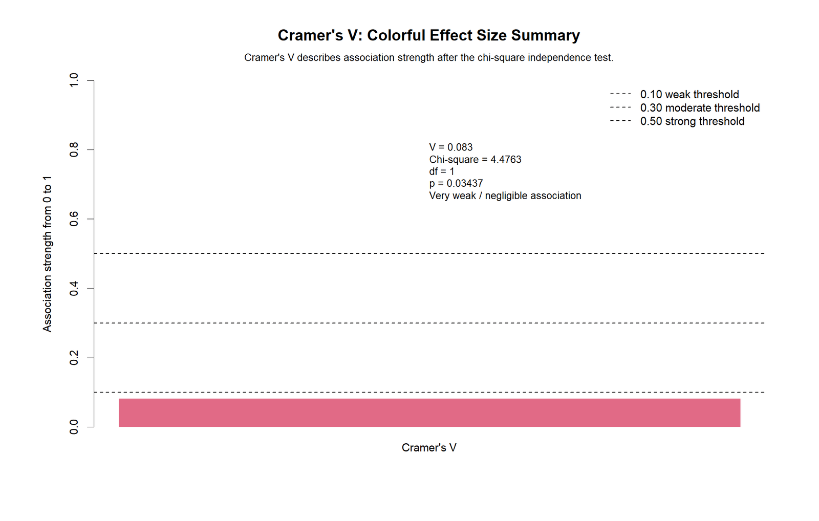
The R effect size summary confirms Cramer’s V = 0.083, χ² = 4.4763, df = 1 and p = 0.03437. The chart labels the result as a very weak or negligible association.
SPSS Output Interpretation
The SPSS output provides the formal crosstabulation, chi-square test and symmetric measures table. It confirms that there were 649 valid cases and no missing cases for the selected school by sex table.
Open the SPSS Cramer’s V Output PDF
| SPSS Output Item | Value | Interpretation |
|---|---|---|
| Valid cases | 649 | All cases were used in the crosstabulation. |
| Pearson Chi-Square | 4.476 | Observed counts differ from expected counts. |
| df | 1 | The table is 2 × 2. |
| Asymptotic significance | .034 | The association is statistically significant at .05. |
| Minimum expected count | 92.63 | No expected-count warning problem; all expected counts are above 5. |
| Phi | -.083 | Signed 2 × 2 association measure; sign depends on coding/order. |
| Cramer’s V | .083 | Unsigned effect size; very weak/negligible strength. |
The SPSS conclusion is that the chi-square test is significant, but Cramer’s V is very small. For reporting, use the Cramer’s V value as the practical strength measure and avoid exaggerating the association.
Excel Worked File Explanation
The Excel workbook is a fully worked formula file for Cramer’s V. It contains the observed table, expected counts, chi-square terms, row and column percentages and final worked solution.
Download the Cramer’s V Fully Worked Excel File
| Excel Sheet | Purpose | Main Formula Idea |
|---|---|---|
| Read Me | Explains the workbook purpose, formulas and effect size guide. | Overview and instructions. |
| Observed Table | Stores the 2 × 2 observed count table. | Edit only the observed count cells if replacing the example. |
| Expected Counts | Calculates independence expectations. | Row total × column total / grand total. |
| Chi-Square Terms | Calculates each cell contribution. | (Observed − Expected)² / Expected. |
| Percentages | Shows row and column percentage profiles. | Observed count divided by row or column total. |
| Worked Solution | Shows final χ², df, p-value, Cramer’s V and interpretation. | CHISQ.DIST.RT and SQRT formulas. |
The workbook result is χ² = 4.476302, df = 1, p = 0.034368, Cramer’s V = 0.083050 and bias-corrected Cramer’s V = 0.073228. The decision is “Significant association,” but the effect size interpretation is “Very weak/negligible.”
Python, R, SPSS and Excel Workflows
| Software | Main Workflow | Best Use |
|---|---|---|
| Python | Use pandas for crosstab, scipy for chi-square, and manual formula for Cramer’s V. | Automated charts, heatmaps and reproducible reports. |
| R | Use table(), chisq.test(), manual Cramer’s V formula and ggplot charts. | Statistical validation and colorful publication charts. |
| SPSS | Use Crosstabs with Chi-square and Phi and Cramer’s V selected. | Formal output PDF and thesis-style tables. |
| Excel | Use observed counts, expected counts, chi-square terms, CHISQ.DIST.RT and SQRT. | Fully worked formula learning and manual checking. |
Code Blocks and Excel Formulas
Python Code for Cramer’s V
import pandas as pd
import numpy as np
from scipy.stats import chi2_contingency

df = pd.read_csv("dataset.csv")

row_var = "school"
col_var = "sex"

observed = pd.crosstab(df[row_var], df[col_var])
chi2, p_value, dof, expected = chi2_contingency(observed, correction=False)

n = observed.values.sum()
rows, cols = observed.shape
min_dim = min(rows - 1, cols - 1)

cramers_v = np.sqrt(chi2 / (n * min_dim))

# Bias-corrected Cramer's V
phi2 = chi2 / n
phi2_corr = max(0, phi2 - ((cols - 1) * (rows - 1)) / (n - 1))
rows_corr = rows - ((rows - 1) ** 2) / (n - 1)
cols_corr = cols - ((cols - 1) ** 2) / (n - 1)
cramers_v_corrected = np.sqrt(phi2_corr / min(cols_corr - 1, rows_corr - 1))

print("Observed counts:")
print(observed)
print("Expected counts:")
print(pd.DataFrame(expected, index=observed.index, columns=observed.columns))
print("Chi-square:", chi2)
print("df:", dof)
print("p-value:", p_value)
print("Cramer's V:", cramers_v)
print("Bias-corrected Cramer's V:", cramers_v_corrected)
R Code for Cramer’s V
df <- read.csv("dataset.csv", stringsAsFactors = FALSE)

row_var <- "school"
col_var <- "sex"

observed <- table(df[[row_var]], df[[col_var]])
test <- chisq.test(observed, correct = FALSE)

chi_square <- unname(test$statistic)
p_value <- test$p.value
df_chi <- unname(test$parameter)
n <- sum(observed)

rows <- nrow(observed)
cols <- ncol(observed)
min_dim <- min(rows - 1, cols - 1)

cramers_v <- sqrt(chi_square / (n * min_dim))

# Bias correction
phi2 <- chi_square / n
phi2_corr <- max(0, phi2 - ((cols - 1) * (rows - 1)) / (n - 1))
rows_corr <- rows - ((rows - 1)^2) / (n - 1)
cols_corr <- cols - ((cols - 1)^2) / (n - 1)
cramers_v_corrected <- sqrt(phi2_corr / min(cols_corr - 1, rows_corr - 1))

print(observed)
print(test$expected)
cat("Chi-square =", chi_square, "\n")
cat("df =", df_chi, "\n")
cat("p-value =", p_value, "\n")
cat("Cramer's V =", cramers_v, "\n")
cat("Bias-corrected Cramer's V =", cramers_v_corrected, "\n")
SPSS Syntax for Cramer's V
* Cramer's V in SPSS.
OUTPUT CLOSE ALL.
OUTPUT NEW NAME=Cramers_V_Output.

CROSSTABS
  /TABLES=school BY sex
  /FORMAT=AVALUE TABLES
  /STATISTICS=CHISQ PHI
  /CELLS=COUNT EXPECTED ROW COLUMN TOTAL RESID SRESID
  /COUNT ROUND CELL.

OUTPUT EXPORT
  /CONTENTS EXPORT=VISIBLE
  /PDF DOCUMENTFILE='Cramers-V-SPSS-Output.pdf'.
Excel Formula Patterns for Cramer's V
Expected count:
=Row_Total*Column_Total/Grand_Total

Chi-square cell term:
=(Observed-Expected)^2/Expected

Total chi-square:
=SUM(all_chi_square_terms)

Degrees of freedom:
=(Rows-1)*(Columns-1)

p-value:
=CHISQ.DIST.RT(Chi_Square, Degrees_of_Freedom)

Minimum dimension:
=MIN(Rows-1, Columns-1)

Cramer's V:
=SQRT(Chi_Square/(N*Minimum_Dimension))

Decision:
=IF(p_value<0.05,"Significant association","Not significant")

Effect size:
=IF(V<0.10,"Very weak/negligible",IF(V<0.30,"Weak",IF(V<0.50,"Moderate","Strong")))
How to Report Cramer's V
A good Cramer's V report should include the variables, contingency table context, chi-square statistic, degrees of freedom, p-value, Cramer's V value and effect size interpretation.
APA-style report: A chi-square test of independence was conducted to examine the association between school and sex. The association was statistically significant, χ²(1, N = 649) = 4.476, p = .034. However, the effect size was very weak, Cramer's V = .083, indicating a negligible association between school and sex.
Expanded interpretation: GP had 237 female and 186 male students, while MS had 146 female and 80 male students. Row percentages showed that MS had a slightly higher female percentage than GP. The chi-square result was statistically significant, but Cramer's V showed that the practical association was very small.
Common Mistakes in Cramer's V Interpretation
| Mistake | Why It Is a Problem | Better Practice |
|---|---|---|
| Reporting only p-value | p-value does not show association strength. | Report chi-square and Cramer's V together. |
| Calling a weak effect strong because p < .05 | Statistical significance can occur with small effects in large samples. | Use effect size wording based on V. |
| Using Pearson correlation for nominal categories | Nominal categories are not continuous variables. | Use chi-square and Cramer's V for categorical association. |
| Ignoring expected counts | Low expected counts can affect chi-square validity. | Check expected counts and Fisher's Exact Test when needed. |
| Overinterpreting residuals | Small residuals do not support strong cell-level claims. | Use residuals to explain the pattern cautiously. |
| Confusing Phi and Cramer's V | Phi is common for 2 × 2 tables; Cramer's V generalizes to larger tables. | Report Cramer's V for general nominal association. |
Downloads and Resources
Download R Report PDFR Cramer's V validation report with colorful charts.
Download SPSS Output PDFSPSS crosstabs, chi-square test and symmetric measures output.
Download Excel Worked FileFormula-based workbook for expected counts, chi-square and Cramer's V.
Open R Effect Size SummaryColorful Cramer's V effect size chart.
External References
For software documentation, see SciPy's chi-square contingency documentation, R's chisq.test documentation and IBM SPSS Crosstabs documentation.
FAQs About Cramer's V
What is Cramer's V?
Cramer's V is an effect size measure for association between two categorical variables. It is based on the chi-square statistic and ranges from 0 to 1.
What was the Cramer's V result in this example?
The result was Cramer's V = 0.08305, with χ²(1) = 4.4763 and p = 0.03437. The association was statistically significant but very weak.
How do I interpret Cramer's V?
A value near 0 indicates weak association. In this guide, V = 0.083 is below 0.10, so it is interpreted as very weak or negligible.
Is Cramer's V the same as chi-square?
No. The chi-square test checks whether an association is statistically significant. Cramer's V measures how strong that association is.
Can Excel calculate Cramer's V?
Yes. Excel can calculate expected counts, chi-square terms, the p-value with CHISQ.DIST.RT and Cramer's V with the SQRT formula.
Should I report bias-corrected Cramer's V?
You can report it as an optional corrected effect size, especially for small samples or larger tables. In this example, the corrected value is 0.07323, still very weak.

