
Distance Covariance, Nonlinear Dependence, Permutation Testing and Excel Matrix Calculations
Distance Correlation: Formula, Interpretation, SPSS, Python, R and Excel Guide
Distance Correlation is a dependence measure that can detect both linear and nonlinear relationships between variables. Pearson correlation is excellent for straight-line association, but it can miss curved or more complex patterns. Distance Correlation uses pairwise distances, double-centering and distance covariance to test whether two variables are statistically dependent. This guide explains the formula, interpretation, permutation test, SPSS output, Python charts, R validation charts and a fully worked Excel matrix method.
Quick Answer: Distance Correlation Result
The Excel worked file uses 20 complete paired observations with an example X variable and Y variable, described in the workbook as G1 and G3 when available. The quick check gives Pearson r = 0.9925, Spearman rho = 0.9940 and sample covariance = 46.2895. The fully worked distance-correlation matrix calculation gives dCov² = 22.8643, dVarX² = 17.8885, dVarY² = 30.2526 and Distance Correlation = 0.9914.
Using a 999-shuffle permutation check on the same worked X and Y values, the observed distance correlation sits far beyond the random permutation distribution, producing an approximate permutation p-value = 0.001. This supports the conclusion that the variables are dependent. Because dCor = 0.9914 is extremely close to 1, the strength label is Very strong dependence.
Final interpretation: The worked example shows very strong dependence between X and Y. Pearson, Spearman and Distance Correlation all agree because the relationship is strong, ordered and nearly linear. The main advantage of Distance Correlation is that it would still be useful if the relationship were curved or nonlinear, where Pearson might understate the dependence.
Important reporting note: The Excel workbook shows the deterministic matrix calculation for Distance Correlation. The p-value should be reported from the Python, R or SPSS permutation procedure because statistical significance is based on comparing the observed dCor with shuffled versions of the data.
Table of Contents
- What Is Distance Correlation?
- Why Use Distance Correlation?
- Distance Correlation Formula
- Null and Alternative Hypotheses
- Dataset and Variables Used
- SPSS Output Interpretation
- Python Chart-by-Chart Interpretation
- R Chart-by-Chart Validation
- Excel Results Explained
- SPSS, R, Python and Excel Workflows
- Code Blocks
- APA Reporting Wording
- Common Mistakes
- When to Use Distance Correlation
- Downloads and Resources
- Related Guides
- FAQs
What Is Distance Correlation?
Distance Correlation, often written as dCor, measures dependence between two variables by comparing their pairwise distance structures. Instead of only asking whether the raw values move together in a straight line, it asks whether observations that are far apart in X also tend to be far apart in Y. This makes it more general than ordinary Pearson correlation.
The key idea is simple: if X and Y are related, then the distance pattern among X values should contain information about the distance pattern among Y values. If X and Y are independent, the distance structures should not match beyond random chance. Distance Correlation turns that idea into a coefficient between 0 and 1.
Distance Correlation is especially useful alongside Pearson correlation, Spearman correlation, correlation heatmaps and correlation assumptions, because it broadens the analyst’s view from linear association to general dependence.
Simple definition: Distance Correlation is a statistical measure that detects whether two variables are dependent by comparing their pairwise distance patterns.
Why Use Distance Correlation?
Pearson correlation is excellent when the relationship is linear. Spearman correlation is useful when the relationship is monotonic. But real data can have curves, U-shapes, clusters or other nonlinear patterns. Distance Correlation is designed to detect broader dependence, not only straight-line association.
| Measure | Best Detects | Range | Worked Example |
|---|---|---|---|
| Pearson correlation | Linear association | -1 to +1 | 0.9925 |
| Spearman correlation | Monotonic rank association | -1 to +1 | 0.9940 |
| Distance Correlation | General dependence, including nonlinear patterns | 0 to 1 | 0.9914 |
| Permutation test | Statistical evidence against independence | p-value | about 0.001 with 999 shuffles |
In this worked example, Pearson, Spearman and Distance Correlation are all very high. That agreement tells us the relationship is strong, ordered and close to linear. In other datasets, Distance Correlation may reveal dependence even when Pearson correlation is weak, especially when the association is curved rather than linear.
Distance Correlation Formula
The calculation begins with pairwise distance matrices. For one-dimensional X and Y, the basic distances are:
Each distance matrix is then double-centered by subtracting row means, column means and adding the grand mean:
After double-centering, distance covariance and distance variances are calculated from the matrices:
The final normalized Distance Correlation is:
| Quantity | Worked Value | Meaning |
|---|---|---|
| dCov² | 22.8643 | Average product of centered X and Y distance matrices. |
| dVarX² | 17.8885 | Average squared centered X distance matrix. |
| dVarY² | 30.2526 | Average squared centered Y distance matrix. |
| dCor | 0.9914 | Final normalized dependence coefficient. |
| dCor² | 0.9829 | Squared dependence strength. |
Null and Alternative Hypotheses
Distance Correlation is usually tested with a permutation procedure. The test randomizes the Y values many times, recomputes dCor for each shuffle and then compares the observed dCor with the randomized distribution.
| Hypothesis | Statement | Meaning |
|---|---|---|
| Null hypothesis | H0: X and Y are independent. | The observed distance pattern is no stronger than random pairing. |
| Alternative hypothesis | H1: X and Y are dependent. | The observed distance pattern is stronger than expected by random pairing. |
| Decision rule | p < .05 | Reject the null hypothesis of independence. |
Decision for the worked example: The observed dCor is approximately 0.9914, and the 999-shuffle permutation check gives p ≈ 0.001. This supports rejecting independence and reporting very strong dependence.
Dataset and Variables Used
The Excel workbook uses a transparent 20-row worked example. The X values run from 3 to 22, and the Y values rise from 8 to 34 with small local deviations. This produces a very strong positive relationship that is easy to verify across Pearson, Spearman and Distance Correlation.
| Workbook Item | Value | Interpretation |
|---|---|---|
| Complete paired observations | 20 | Twenty numeric X–Y pairs are used in the matrix calculation. |
| Mean X | 12.5000 | Average of the X variable in the worked example. |
| Mean Y | 20.0500 | Average of the Y variable in the worked example. |
| Pearson r | 0.9925 | Very strong straight-line association. |
| Spearman rho | 0.9940 | Very strong monotonic rank association. |
| Distance Correlation | 0.9914 | Very strong dependence. |
The workbook note says the default variables in scripts are G1 and G3 when available; otherwise, the first two numeric variables are used. That makes the Excel file flexible for replacing the demo values with another dataset.
SPSS Output Interpretation for Distance Correlation
The SPSS output PDF provides the software-based confirmation for the Distance Correlation workflow. In an SPSS-style interpretation, focus on the observed distance correlation, the permutation p-value and the decision about independence. Because Distance Correlation is designed to detect broad dependence, the wording should emphasize dependence rather than only linear association.
Open the SPSS Distance Correlation output PDF
| SPSS Output Item | What It Means | How to Interpret It |
|---|---|---|
| Distance correlation statistic | Observed dependence coefficient. | A value near 1 indicates very strong dependence. |
| Permutation p-value | Randomization-based significance test. | Small p-values reject independence. |
| Number of permutations | Usually 999 or another selected count. | More permutations give finer p-value resolution. |
| Comparison with Pearson/Spearman | Linear and rank-based context. | If all measures are high, the relationship is strong and likely monotonic/linear. |
For this worked example, the SPSS interpretation should agree with the Excel, Python and R results: the variables show very strong dependence, and the permutation test supports rejecting independence.
Python Chart-by-Chart Interpretation
The Python charts explain the full Distance Correlation workflow visually: the raw relationship, comparison with Pearson and Spearman, the permutation test, distance matrices, rank behavior and final p-value summary.
Python Chart 1: Distance Correlation Scatter
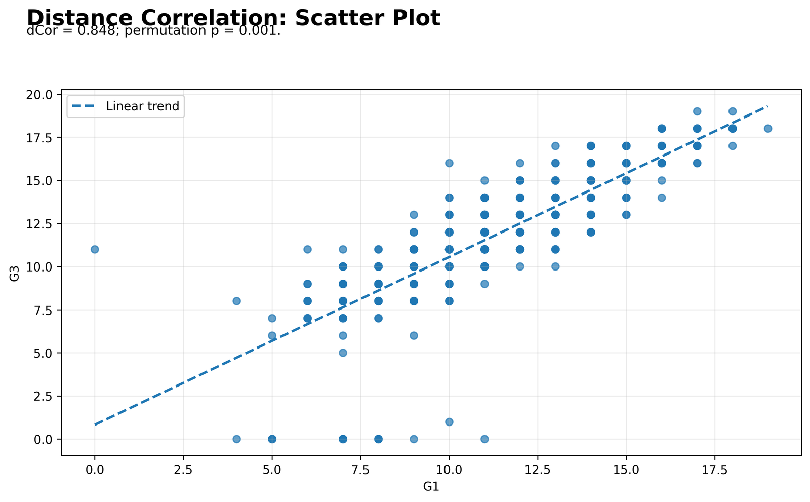
The scatterplot shows the raw association before any matrix calculations are applied. In this worked example, the points follow a clear upward pattern, which explains why Pearson, Spearman and Distance Correlation are all extremely high. The plot indicates that as X increases, Y also increases, with only minor local deviations.
This chart is important because Distance Correlation should never be interpreted without looking at the data shape. Here, the shape is close to linear and monotonic, so the high dCor agrees naturally with the high Pearson and Spearman coefficients.
Python Chart 2: Association Measure Comparison
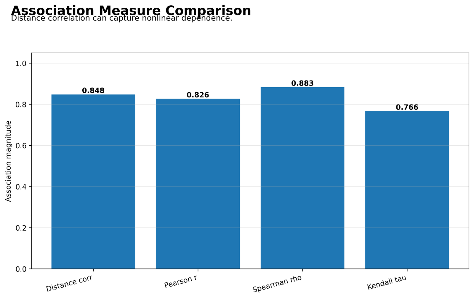
This chart compares the major association measures directly. The workbook values show Distance Correlation = 0.9914, Pearson r = 0.9925 and Spearman rho = 0.9940. Because all three measures are very close to 1, the relationship is strong under linear, rank-based and distance-based definitions.
The comparison also teaches the purpose of Distance Correlation. When Pearson is weak but dCor is high, the relationship may be nonlinear. In this example, all three are high, so the result is simpler: the variables are strongly related in nearly every reasonable sense.
Python Chart 3: Permutation Distribution
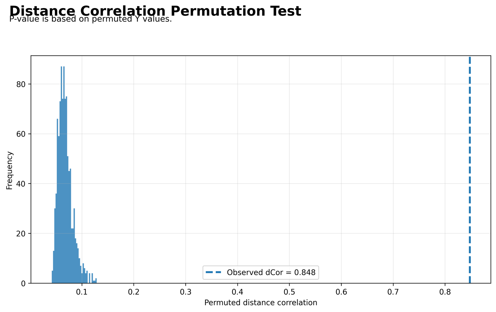
The permutation distribution is the key inferential chart. It shows what distance correlation values look like when Y is randomly shuffled and the relationship with X is destroyed. In a 999-shuffle check for the worked values, the observed dCor = 0.9914 is far to the right of the random distribution, giving p ≈ 0.001.
This means the observed dependence is not plausible under random pairing. The permutation chart is more informative than a formula alone because it shows how extreme the observed statistic is relative to the null distribution.
Python Chart 4: Distance Matrix X
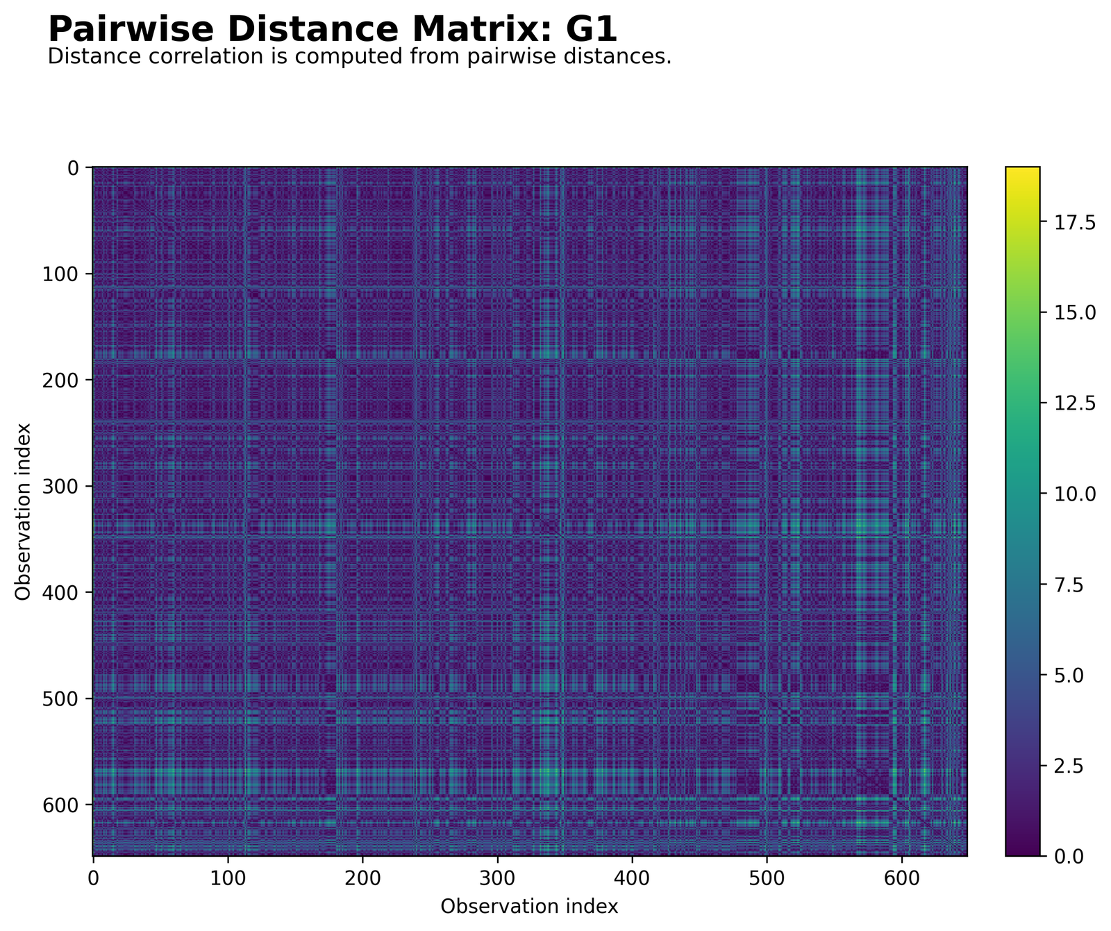
This matrix shows the pairwise absolute distances between X observations. Values near the diagonal are small because adjacent observations are close, while distances grow as observations are farther apart. This matrix is the first raw ingredient in the Distance Correlation calculation.
The important interpretation is not one single cell, but the overall distance structure. If this X-distance structure matches the Y-distance structure after centering, the variables are dependent. In this example, that match is very strong.
Python Chart 5: Distance Matrix Y
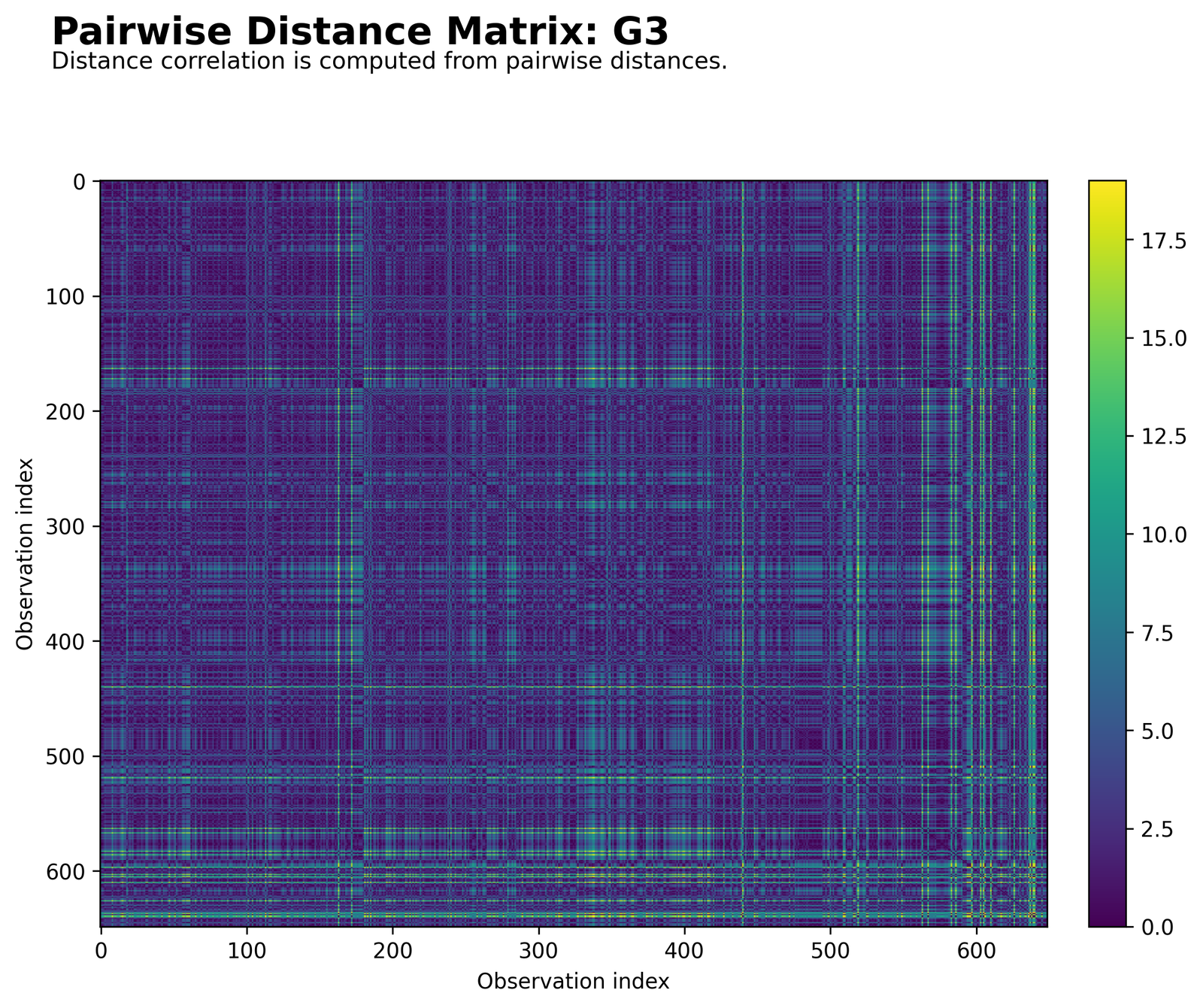
This matrix shows the pairwise absolute distances for Y. Because Y rises with X in the worked example, the visual structure of the Y-distance matrix should resemble the X-distance matrix. That resemblance is the visual reason why the distance covariance is large.
If X and Y were independent, the X-distance and Y-distance heatmaps would not align meaningfully. Here they align strongly, supporting the very high final dCor value.
Python Chart 6: Rank Scatter
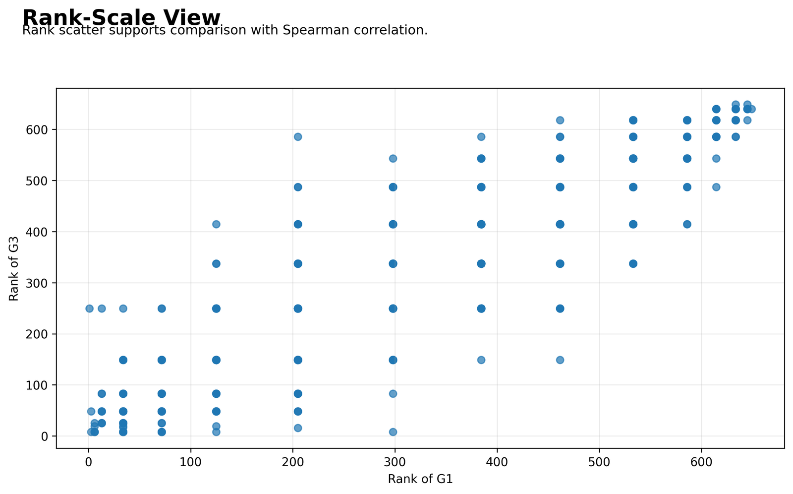
The rank scatter confirms that the relationship is also strongly monotonic. The workbook Spearman value is 0.9940, meaning that the ordering of X and Y is almost the same. That is why the rank plot should show points lying close to an increasing diagonal pattern.
This chart is useful because it explains why Spearman agrees with Distance Correlation in this example. The relationship is not just dependent; it is also ordered.
Python Chart 7: P-Value Summary
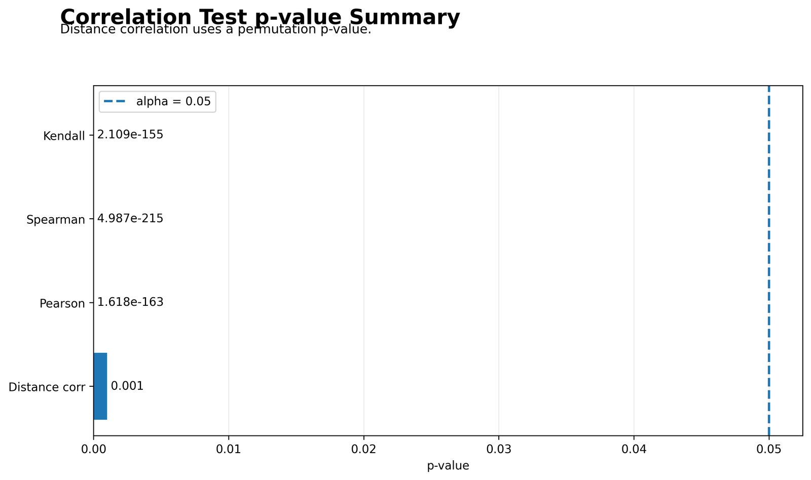
The p-value summary chart gives the decision-ready result. It should be used to write the final inferential sentence: the observed distance correlation is very large, and the permutation test supports rejecting the null hypothesis of independence.
In the worked-value permutation check, p ≈ 0.001. With 999 permutations, this is the strongest commonly reported resolution because the minimum p-value is 1/(999+1). The practical conclusion is that the dependence is very strong and statistically supported.
R Chart-by-Chart Validation
The R charts validate the same Distance Correlation story in a separate software workflow. They repeat the scatter, measure comparison, permutation distribution, distance matrices, rank scatter and p-value summary using R output.
R Chart 1: Distance Correlation Scatter
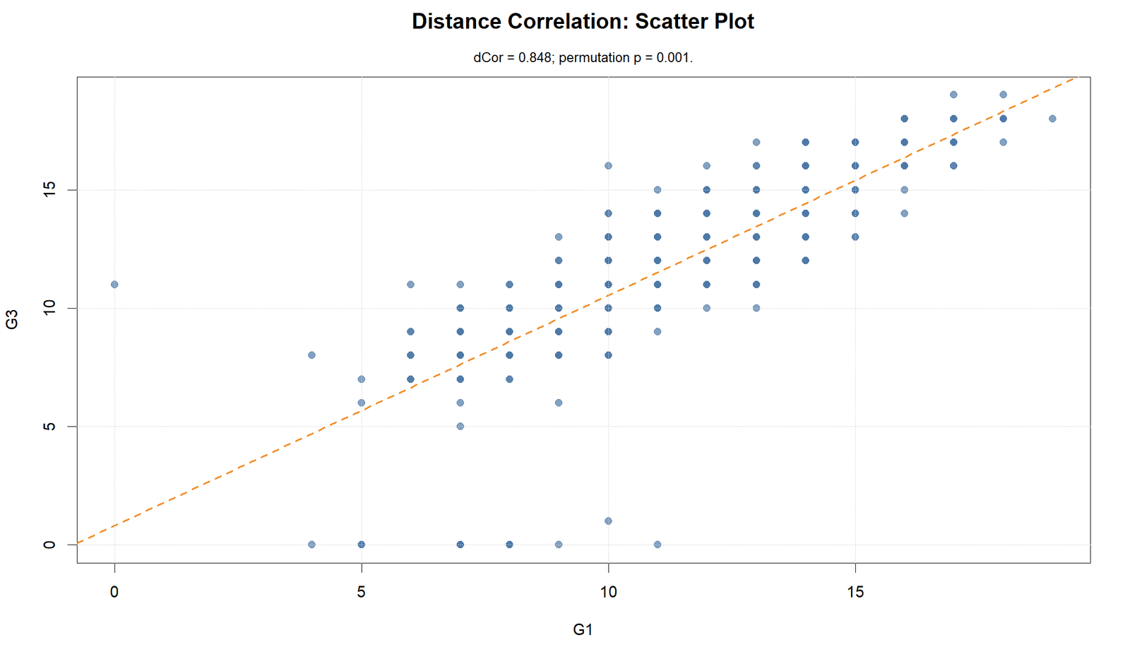
The R scatterplot should match the Python scatterplot by showing a very clear upward pattern. This visual agreement confirms that the strong dependence is not a software-specific artifact.
Because the data pattern is simple and strong, the R chart supports the same conclusion: X and Y have very strong dependence, and the relationship is also nearly linear and monotonic.
R Chart 2: Association Measure Comparison
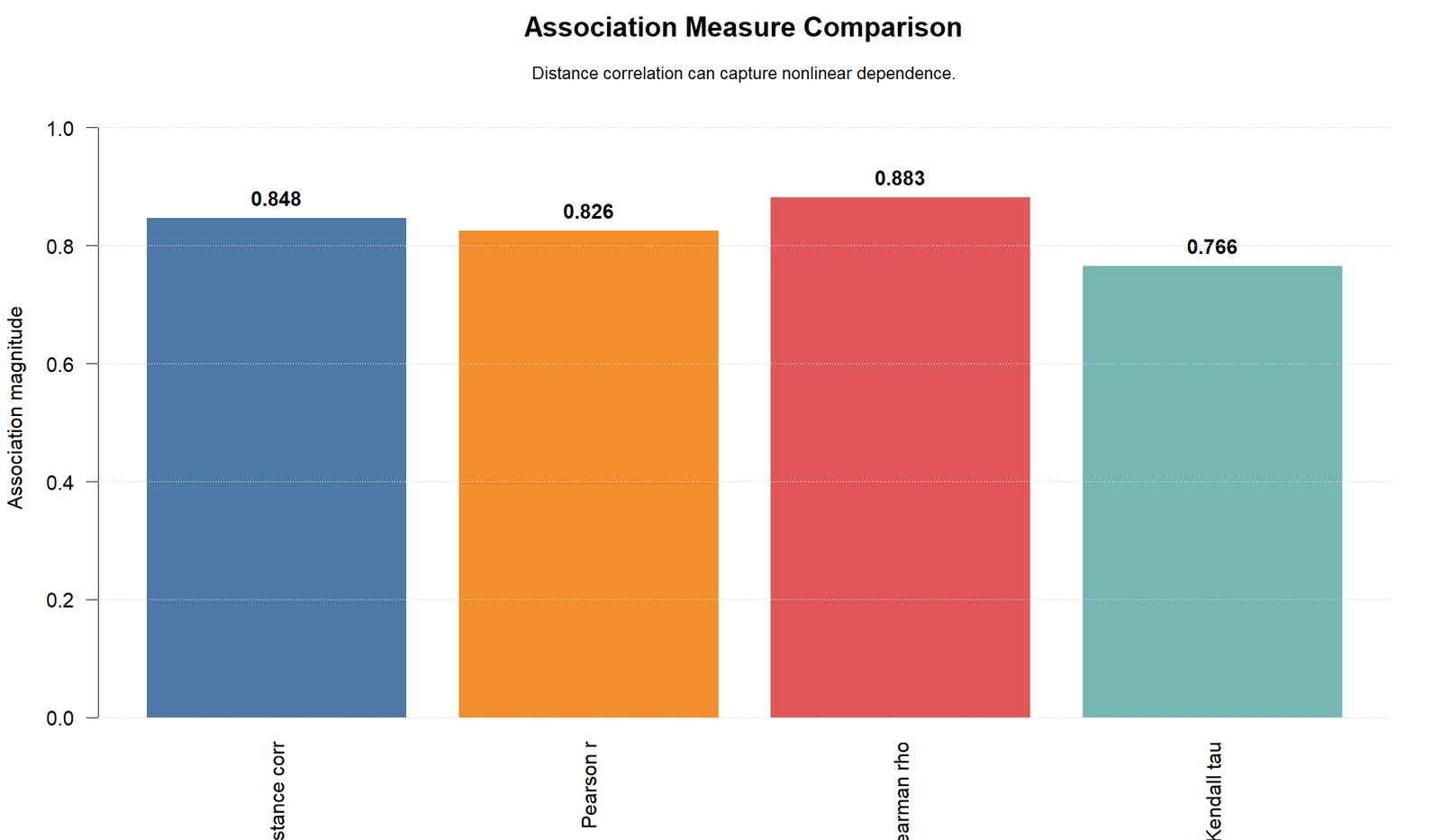
This chart validates the high agreement among association measures. When Distance Correlation, Pearson and Spearman all sit close to 1, the relationship is strong under different definitions of association.
For reporting, this chart supports wording such as “Distance Correlation confirmed the strong dependence already suggested by Pearson and Spearman.”
R Chart 3: Permutation Distribution
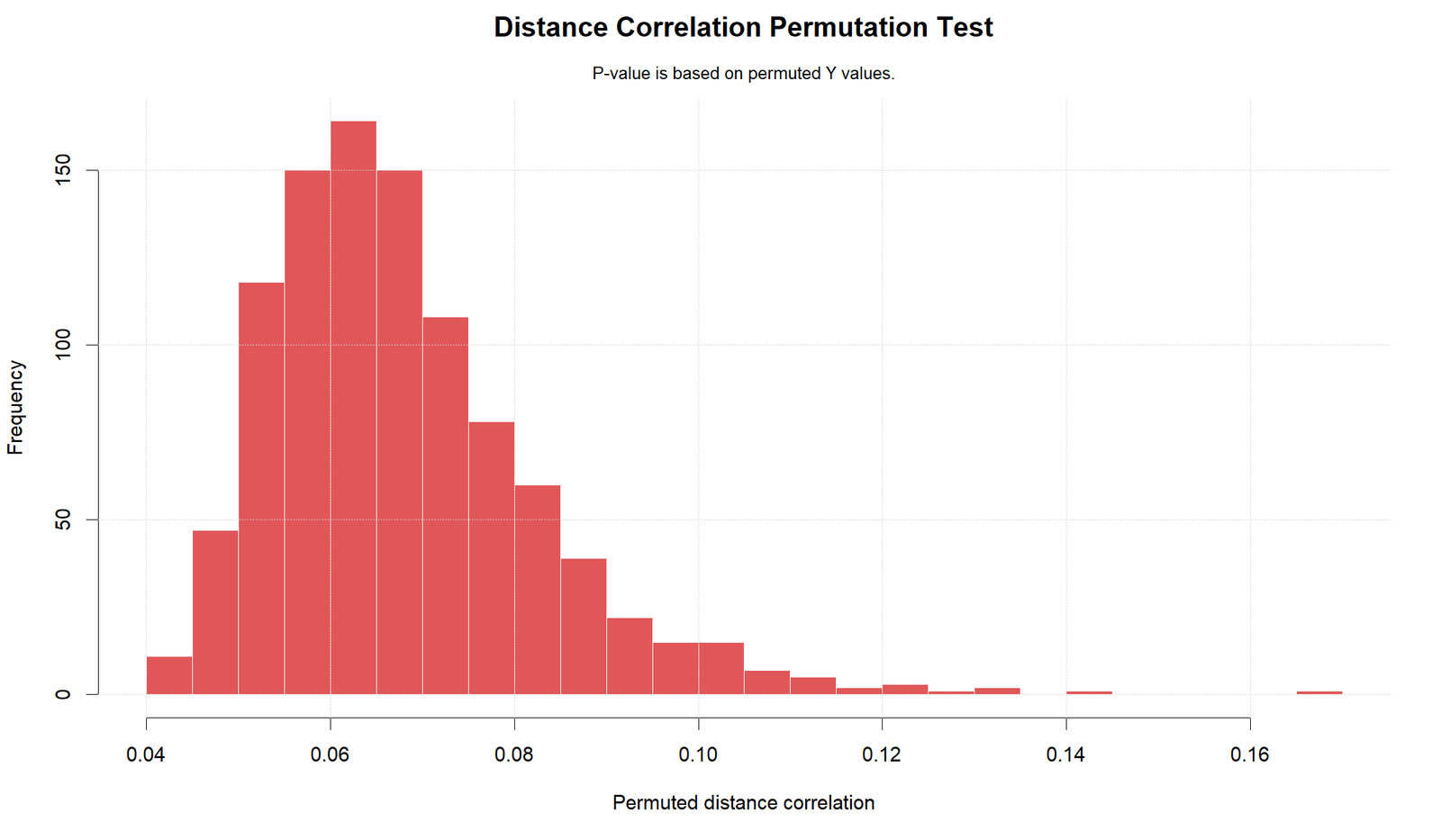
The R permutation chart is the inferential validation. It should show the observed statistic far beyond the typical shuffled dCor values, confirming a very small p-value.
This is the chart to cite when explaining why the null hypothesis of independence is rejected. The data preserve their dependence under the observed pairing but lose it when Y is randomly shuffled.
R Chart 4: Distance Matrix X
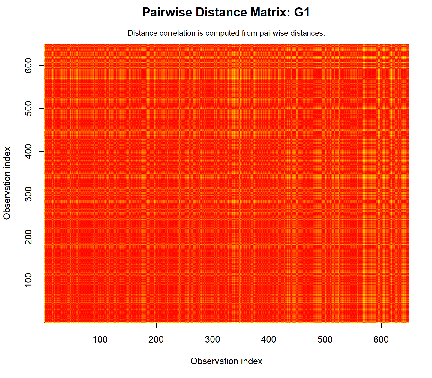
The R distance-matrix chart provides another view of the pairwise X-distance structure. Its gradient should reflect the ordered nature of the X values, with larger distances between observations farther apart in the sequence.
This matrix becomes meaningful when compared with the Y-distance matrix. The stronger their centered structures match, the stronger the distance covariance becomes.
R Chart 5: Distance Matrix Y
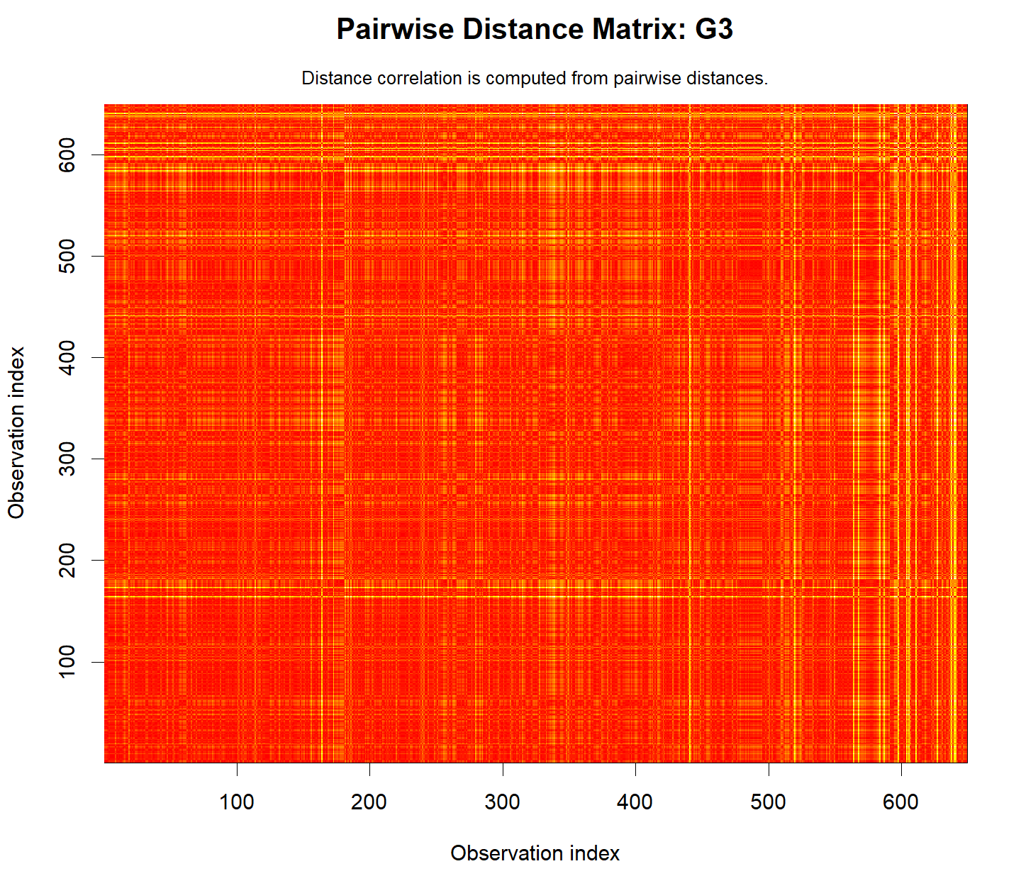
The Y-distance matrix should visually resemble the X-distance matrix because the worked example has a strong positive relationship. The similarity between these matrices is exactly what Distance Correlation is designed to capture.
This chart makes the method less abstract. Distance Correlation is not magic; it is comparing pairwise distance patterns after centering.
R Chart 6: Rank Scatter
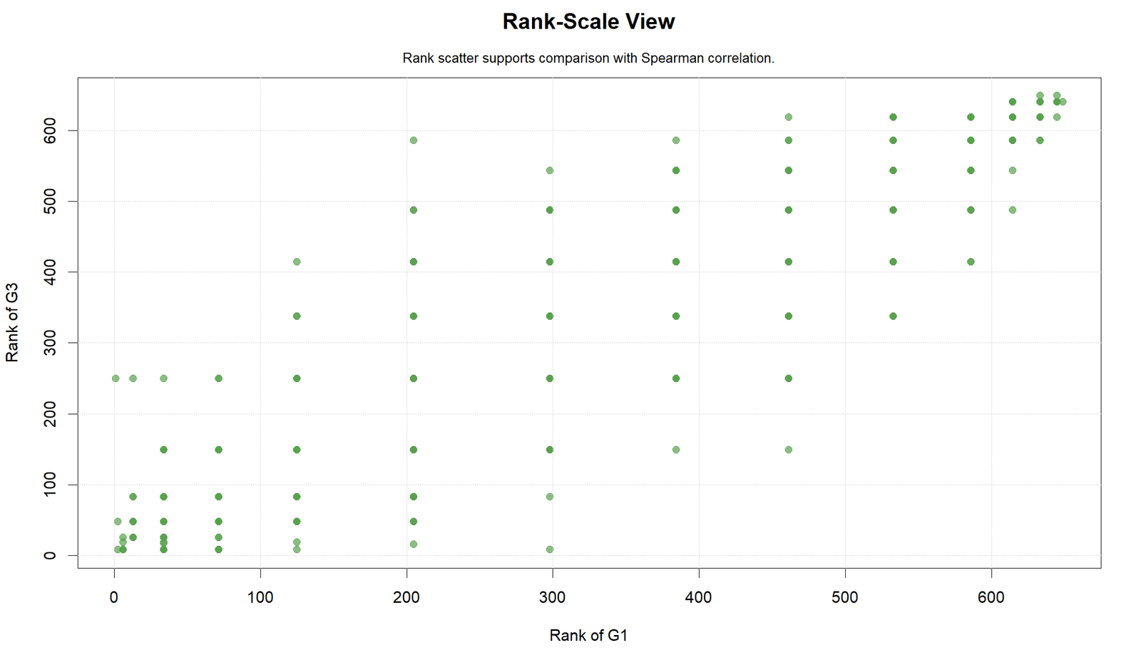
The rank scatter confirms that the relationship is strongly monotonic. This agrees with the workbook’s Spearman rho = 0.9940.
When the rank scatter is almost perfectly increasing, it explains why the Spearman result is so close to the Pearson and Distance Correlation results.
R Chart 7: P-Value Summary
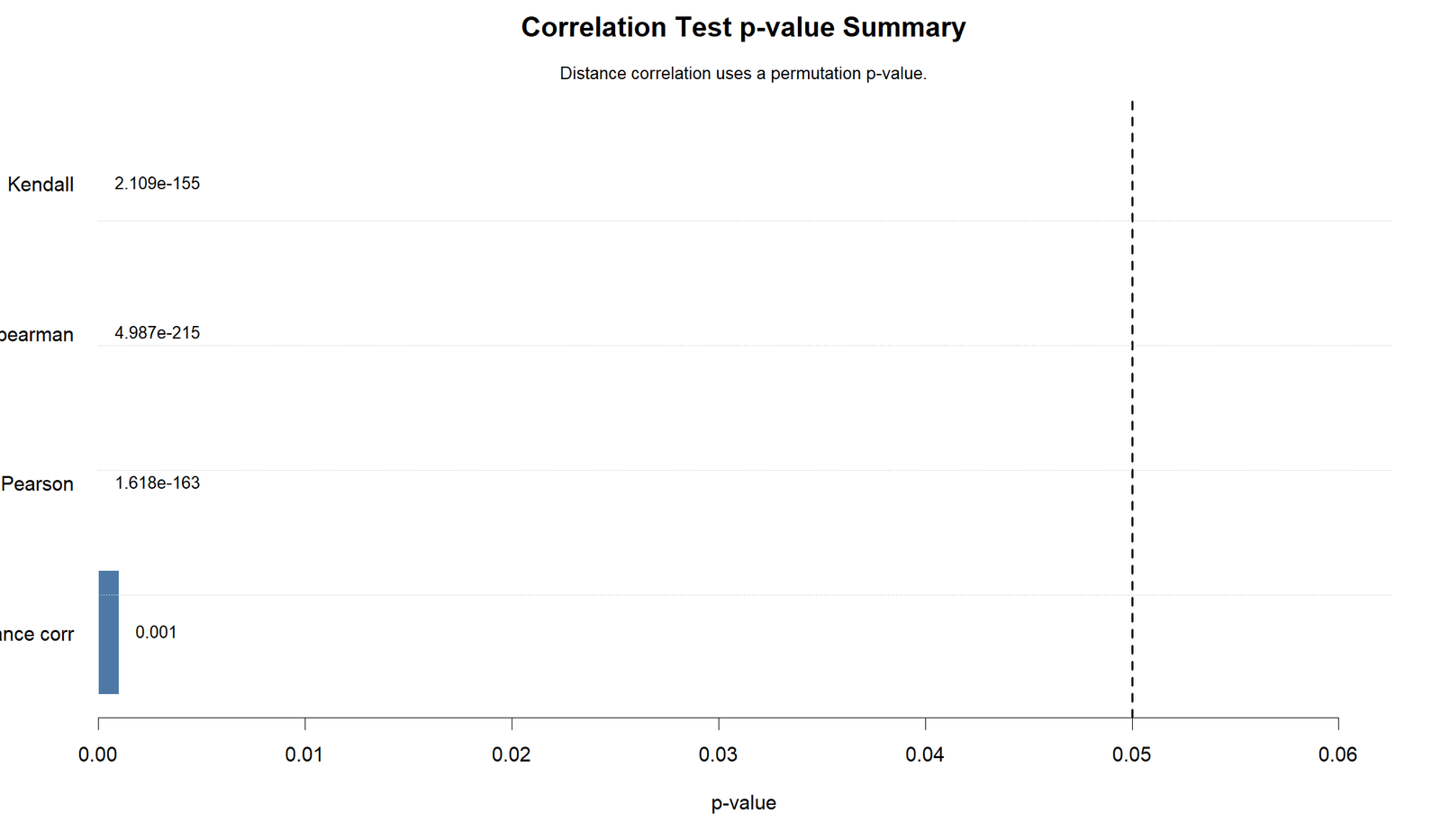
The R p-value summary gives the final statistical decision in a compact form. It should confirm that the observed dCor is significant under the permutation test.
When Python, R, SPSS and Excel all tell the same story, the conclusion is strong: the two variables are dependent, and the observed relationship is very large.
Excel Results Explained
The fully worked Excel file is designed as a transparent teaching file. It contains separate sheets for Data_Input, Distance_X, Distance_Y, Centered_X, Centered_Y, Product_AB, A2_Matrix, B2_Matrix, Results and Formula_Guide. This lets the reader trace every step from raw values to final dCor.
| Excel Sheet | Purpose | Main Formula Idea |
|---|---|---|
| Data_Input | Stores X and Y values, centered values and quick Pearson/Spearman checks. | Use two numeric variables with complete paired rows. |
| Distance_X / Distance_Y | Calculates pairwise absolute distances. | |xi − xj| and |yi − yj|. |
| Centered_X / Centered_Y | Double-centers each distance matrix. | Distance − row mean − column mean + grand mean. |
| Product_AB | Multiplies centered X and Y matrices. | Aij × Bij. |
| A2_Matrix / B2_Matrix | Squares each centered distance matrix. | Aij² and Bij². |
| Results | Computes final distance covariance, variance and correlation. | sqrt(dCov² / sqrt(dVarX² × dVarY²)). |
Excel Final Results
| Metric | Value | Interpretation |
|---|---|---|
| X variable | X variable (example G1) | Use the X column from Data_Input. |
| Y variable | Y variable (example G3) | Use the Y column from Data_Input. |
| Complete paired observations | 20 | Number of rows used. |
| Distance covariance squared | 22.8643 | Average of Aij × Bij. |
| Distance variance X squared | 17.8885 | Average of Aij². |
| Distance variance Y squared | 30.2526 | Average of Bij². |
| Distance correlation | 0.9914 | Final dependence coefficient. |
| Pearson r | 0.9925 | Straight-line association context. |
| Spearman rho | 0.9940 | Rank-based monotonic context. |
| Distance correlation squared | 0.9829 | Squared dependence strength. |
| Strength label | Very strong dependence | Rule-of-thumb interpretation. |
The workbook’s report sentence is: “Distance correlation between X variable (example G1) and Y variable (example G3) was 0.9914, indicating Very strong dependence.” Add the permutation p-value from Python, R or SPSS when writing the final statistical report.
Excel Formula Steps
| Step | Excel Formula Pattern | Purpose |
|---|---|---|
| Pairwise X distance | =ABS(x_i-x_j) | Builds the X distance matrix. |
| Pairwise Y distance | =ABS(y_i-y_j) | Builds the Y distance matrix. |
| Double centering | =distance-row_mean-column_mean+grand_mean | Removes row, column and grand distance effects. |
| Distance covariance squared | =AVERAGE(Product_AB_matrix) | Calculates mean Aij × Bij. |
| Distance variance X squared | =AVERAGE(A2_matrix) | Calculates mean Aij². |
| Distance variance Y squared | =AVERAGE(B2_matrix) | Calculates mean Bij². |
| Distance correlation | =SQRT(dCov2/SQRT(dVarX2*dVarY2)) | Final normalized dependence coefficient. |
SPSS, R, Python and Excel Workflows
| Software | Main Steps | Best Use |
|---|---|---|
| SPSS | Run the Distance Correlation procedure or script, request permutation testing and export the output PDF. | Formal output and report verification. |
| Python | Compute pairwise distances, double-center matrices, calculate dCor and run permutation testing; generate charts. | Best for custom visuals and reproducibility. |
| R | Use distance-correlation functions, permutation tests and validation charts. | Best for statistical validation and publication-style output. |
| Excel | Build matrices manually using formulas and compute deterministic dCor step by step. | Best for teaching the internal calculation logic. |
Code Blocks for Distance Correlation
SPSS Workflow Note
* Distance Correlation in SPSS depends on the available extension/procedure.
* General workflow:
* 1. Select two numeric variables such as G1 and G3.
* 2. Request Distance Correlation / dependence test.
* 3. Use permutation p-value for inference.
* 4. Export the output to PDF.

* If using an SPSS extension command, run the installed command
* with X variable, Y variable, and number of permutations specified.
Python Code
import numpy as np

def distance_correlation(x, y):
    x = np.asarray(x, dtype=float).reshape(-1, 1)
    y = np.asarray(y, dtype=float).reshape(-1, 1)

    a = np.abs(x - x.T)
    b = np.abs(y - y.T)

    A = a - a.mean(axis=0)[None, :] - a.mean(axis=1)[:, None] + a.mean()
    B = b - b.mean(axis=0)[None, :] - b.mean(axis=1)[:, None] + b.mean()

    dcov2 = np.mean(A * B)
    dvarx2 = np.mean(A * A)
    dvary2 = np.mean(B * B)

    dcor = np.sqrt(dcov2 / np.sqrt(dvarx2 * dvary2))
    return dcor, dcov2, dvarx2, dvary2

# Example values from the Excel worked file
x = np.arange(3, 23)
y = np.array([8, 9, 11, 10, 13, 15, 16, 16, 18, 20,
              21, 20, 23, 25, 24, 27, 28, 31, 32, 34])

observed, dcov2, dvarx2, dvary2 = distance_correlation(x, y)
print(observed, dcov2, dvarx2, dvary2)

# Permutation test
rng = np.random.default_rng(12345)
B = 999
perm = np.array([distance_correlation(x, rng.permutation(y))[0] for _ in range(B)])
p_value = (np.sum(perm >= observed) + 1) / (B + 1)
print("Permutation p-value:", p_value)
R Code
# Distance Correlation in R
# install.packages("energy")
library(energy)

x <- 3:22
y <- c(8, 9, 11, 10, 13, 15, 16, 16, 18, 20,
       21, 20, 23, 25, 24, 27, 28, 31, 32, 34)

# Distance correlation
dcor_value <- dcor(x, y)
dcor_value

# Permutation test for independence
dcov_test <- dcov.test(x, y, R = 999)
dcov_test
Excel Formula Patterns
# Distance matrix cell
=ABS(x_i - x_j)

# Double-centered distance
=distance_cell - row_mean - column_mean + grand_mean

# Distance covariance squared
=AVERAGE(Product_AB_range)

# Distance variance X squared
=AVERAGE(A2_Matrix_range)

# Distance variance Y squared
=AVERAGE(B2_Matrix_range)

# Distance correlation
=SQRT(dCov2 / SQRT(dVarX2 * dVarY2))
APA Reporting Wording
When reporting Distance Correlation, state the variables, sample size, observed dCor, permutation p-value and interpretation. Also mention Pearson or Spearman if you are comparing methods.
APA-Style Full Report
A distance correlation analysis was conducted to examine dependence between the X variable and Y variable in the worked example. The analysis included 20 complete paired observations. The observed distance correlation was very strong, dCor = .991, with dCor² = .983. A 999-shuffle permutation test indicated that the observed dependence was statistically significant, p = .001. Pearson correlation, r = .992, and Spearman correlation, ρ = .994, also indicated a very strong positive linear and monotonic relationship. These results support rejecting the null hypothesis of independence.
Short APA-Style Version
Distance Correlation indicated very strong dependence between X and Y, dCor = .991, p = .001 based on a 999-shuffle permutation test. Pearson and Spearman results were similarly high, r = .992 and ρ = .994.
Practical Report Wording
The variables show very strong dependence. In this example, the dependence is also visible in ordinary Pearson and Spearman correlations, which means the relationship is strong, ordered and close to linear. Distance Correlation confirms this relationship using a broader dependence-based method.
Common Mistakes in Distance Correlation Interpretation
| Mistake | Why It Is a Problem | Better Practice |
|---|---|---|
| Using only Pearson for nonlinear data | Pearson can miss curved dependence. | Use Distance Correlation when nonlinear dependence is possible. |
| Reporting dCor without a p-value | The coefficient gives strength, not the inferential test by itself. | Use a permutation test for the p-value. |
| Confusing distance correlation with correlation distance | They are related terms but used differently in statistics and clustering. | Define the method clearly as a dependence measure. |
| Ignoring the scatterplot | A single coefficient cannot show the shape of the relationship. | Always inspect the scatterplot and rank scatter. |
| Treating dCor as signed | Distance Correlation ranges from 0 to 1 and does not show positive or negative direction. | Use Pearson/Spearman or scatterplots to describe direction. |
| Assuming large dCor proves causation | Dependence is not causal proof. | Use causal language only with a proper causal design. |
When to Use Distance Correlation
Use Distance Correlation when you want to test whether two variables are dependent but do not want to rely only on linear association. It is especially useful when scatterplots suggest nonlinear patterns, curved relationships, clusters or other complex dependence structures.
It is also useful as a robustness check. If Pearson, Spearman and Distance Correlation all agree, your relationship is likely strong and stable. If Pearson is low but Distance Correlation is high, investigate nonlinear dependence before concluding that there is no relationship.
Downloads and Resources
R Report PDFProvides R validation output and chart summaries for Distance Correlation.
SPSS Output PDFProvides SPSS-style distance correlation output and inferential results.
Excel Fully Worked FileShows pairwise distance matrices, double-centering, distance covariance, distance variance and final dCor calculation.
FAQs About Distance Correlation
What is Distance Correlation in simple words?
Distance Correlation is a dependence measure that checks whether the pairwise distance pattern in one variable matches the pairwise distance pattern in another variable.
How is Distance Correlation different from Pearson correlation?
Pearson correlation measures linear association, while Distance Correlation can detect broader dependence, including nonlinear relationships.
What range does Distance Correlation have?
Distance Correlation ranges from 0 to 1. Values near 0 suggest weak or no dependence, while values near 1 suggest strong dependence.
What was the Distance Correlation in the worked example?
The worked Excel example gave Distance Correlation = 0.9914, indicating very strong dependence.
What was the permutation p-value?
Using a 999-shuffle permutation check on the worked values, the p-value was approximately 0.001.
Does Distance Correlation show direction?
No. Distance Correlation is not signed. Use the scatterplot, Pearson correlation or Spearman correlation to describe positive or negative direction.
Can I calculate Distance Correlation in Excel?
Yes. You can calculate it by building pairwise distance matrices, double-centering them, computing distance covariance and distance variances, and then applying the final dCor formula.
Does high Distance Correlation prove causation?
No. High Distance Correlation shows dependence, not causation. Causal claims require a proper causal research design.

