
ANOVA Post Hoc Comparison, Bayesian K-Ratio, SPSS WALLER(100)
Waller Duncan Test: Formula, Interpretation, SPSS, Python, R and Excel Guide
Waller Duncan Test, also called the Waller-Duncan Bayesian K-ratio t test, is a post hoc multiple comparison method used after a significant ANOVA. Unlike many post hoc procedures that focus mainly on controlling Type I error, the Waller Duncan Test uses a K-ratio to express how serious Type I error is compared with Type II error. This guide explains the method with SPSS WALLER(100), Python charts, R validation, Excel workflow, pairwise decisions, ordered group means, homogeneous subset letters, APA reporting and downloadable resources.
Quick Answer: Waller Duncan Test Result
The worked Waller Duncan Test compared four coded groups after a statistically significant ANOVA. The method report card used Waller-Duncan Bayesian K-ratio t test with K-ratio = 100, a reference alpha of 0.05, and a K-ratio alpha approximation of 0.0099. The ANOVA result was F = 15.8763 with p = 0.00000, which should be reported as p < .001, not as p equals zero.
The ordered means were Group 1 = 10.84, Group 2 = 12.09, Group 4 = 13.06, and Group 3 = 13.23. The Waller-Duncan pairwise decision classified 4 of the 6 pairwise comparisons as different. Group 1 was separated from every higher group. Group 3 and Group 4 were not separated from each other, and Group 4 and Group 2 were not separated from each other, but Group 3 and Group 2 were separated. This creates an overlapping homogeneous subset pattern.
Final interpretation: The Waller Duncan Test shows that the group means are not all part of one common performance level. Group 1 is clearly the lowest group. Group 3 is the highest mean group, but it is close enough to Group 4 that those two are not separated by the Waller-Duncan rule. Group 4 also overlaps with Group 2, while Group 3 and Group 2 are separated. A compact letter display can be reported as Group 3 = A, Group 4 = AB, Group 2 = B, and Group 1 = C.
Important reporting point: A Waller Duncan Test result depends on the selected K-ratio. In this example, K = 100 means Type I error is treated as 100 times as serious as Type II error. A different K-ratio can produce a different separation pattern, so the K-ratio should always be reported.
Table of Contents
- What Is the Waller Duncan Test?
- Waller Duncan Test Formula and K-Ratio Logic
- Hypotheses and Decision Rule
- Dataset and Group Means Used
- SPSS Waller Duncan Test Interpretation
- Python Chart-by-Chart Interpretation
- R Chart-by-Chart Validation
- SPSS, R, Python and Excel Workflows
- Code Blocks for Waller Duncan Test
- APA Reporting Wording
- Common Mistakes
- When to Use Waller Duncan Test
- Downloads and Resources
- Related Guides
- FAQs
What Is the Waller Duncan Test?
The Waller Duncan Test is a post hoc comparison method used after an ANOVA indicates that at least one group mean is different. It compares ordered group means and decides which group pairs are far enough apart to be classified as different. The test is often known in SPSS as the Waller-Duncan option or WALLER(K), where K is the seriousness ratio used in the decision rule.
The special feature of the Waller Duncan Test is the K-ratio. The K-ratio represents how serious a Type I error is compared with a Type II error. A Type I error means declaring a difference when the real means are not different. A Type II error means failing to detect a real difference. In a Waller-Duncan framework, the researcher makes this seriousness balance explicit instead of treating all multiple-comparison decisions in the same way.
In this example, the K-ratio is 100. This means the analysis treats Type I error as much more serious than Type II error. The method report card shows the K-ratio alpha approximation as 0.0099, which is stricter than the reference alpha of 0.05. That is why the result should be interpreted as a controlled post hoc separation pattern rather than a simple list of ordinary unadjusted pairwise t tests.
Simple definition: The Waller Duncan Test is an ANOVA post hoc test that uses a K-ratio to decide whether ordered group means should be separated into different homogeneous groups.
The Waller Duncan Test belongs to the post hoc stage of one-way ANOVA. It should be used only after understanding ANOVA assumptions, the F distribution, p-values, effect size, and confidence intervals.
Waller Duncan Test Formula and K-Ratio Logic
The Waller Duncan Test begins with the ANOVA error term. The group means are ordered from low to high, and pairwise mean differences are compared against a K-ratio-based critical difference. The exact critical value is usually produced by statistical software such as SPSS, but the logic can be written in a familiar comparison form.
The standard error for a pairwise mean difference is commonly based on the ANOVA mean square error and the two sample sizes:
The pairwise test statistic can then be expressed as:
The Waller-Duncan decision is made by comparing the observed mean difference or t statistic with the K-ratio critical reference:
| Term | Meaning | Interpretation in Waller Duncan Test |
|---|---|---|
| Mi, Mj | Two group means | The means being compared after ANOVA. |
| MSE | Mean square error | The pooled within-group variance from the ANOVA table. |
| ni, nj | Group sample sizes | Used to calculate the standard error for each pair. |
| K-ratio | Type I / Type II error seriousness ratio | Controls how strict or permissive the Waller-Duncan decision becomes. |
| Critical difference | Required difference for separation | If the observed difference exceeds this value, the pair is classified different. |
| Subset letters | Compact grouping labels | Groups sharing a letter are not separated; groups not sharing a letter are separated. |
Excel caution: Excel can reproduce the learning workflow by calculating means, MSE, standard errors and approximate t decisions, but exact Waller-Duncan critical values are best produced by SPSS or a validated R/Python implementation. For official reporting, use software output such as SPSS WALLER(100).
Hypotheses and Decision Rule for Waller Duncan Test
The Waller Duncan Test is used after the omnibus ANOVA. The ANOVA first tests whether all group means can be treated as equal. If the ANOVA is significant, the Waller-Duncan post hoc test identifies which pairs are separated.
| Stage | Hypothesis or Rule | Meaning |
|---|---|---|
| ANOVA null hypothesis | H0: μ1 = μ2 = μ3 = μ4 | All group population means are equal. |
| ANOVA alternative hypothesis | H1: At least one group mean differs | The omnibus test supports post hoc comparison. |
| Pairwise null hypothesis | H0: μi = μj | The two groups being compared have equal means. |
| Pairwise decision rule | Observed difference > Waller-Duncan critical difference | The pair is classified as different. |
| Homogeneous subset rule | Groups sharing a letter are not separated | Letters summarize the pairwise decision pattern. |
Decision in this example: The ANOVA was significant, F = 15.8763, p < .001. The Waller-Duncan post hoc stage classified 4 of 6 pairwise comparisons as different. The result supports a real ordered mean pattern, but not every pair of adjacent high groups is separated.
Dataset and Group Means Used
The worked example compares four coded groups. The exact group meaning depends on the dataset coding, but the post hoc interpretation is based on the ordered means and pairwise decisions. The group means show a clear upward pattern from Group 1 to Group 3.
| Ordered Position | Group | Mean | Suggested Letter | Interpretation |
|---|---|---|---|---|
| Lowest | Group 1 | 10.84 | C | Lowest mean and separated from all higher groups. |
| Second | Group 2 | 12.09 | B | Higher than Group 1, lower than Groups 4 and 3. |
| Third | Group 4 | 13.06 | AB | Bridge group; overlaps with both Group 2 and Group 3. |
| Highest | Group 3 | 13.23 | A | Highest mean and separated from Group 2 and Group 1. |
This pattern is important because the highest mean alone does not fully explain the result. The Waller Duncan Test shows that Group 3 and Group 4 are statistically close, and Group 4 and Group 2 are also statistically close. Group 4 is therefore an overlapping subgroup, which is why the letter AB is more informative than a simple rank number.
SPSS Waller Duncan Test Interpretation
The SPSS-style result uses the official software reference SPSS WALLER(100). The output is interpreted as a post hoc follow-up to ANOVA. The method report card confirms that the K-ratio is 100, the reference alpha is 0.05, the K-ratio alpha approximation is 0.0099, and the ANOVA is significant.
SPSS Method Summary
| SPSS Output Item | Value | Interpretation |
|---|---|---|
| Method | Waller-Duncan Bayesian K-ratio t test | The post hoc method uses K-ratio seriousness balancing. |
| K-ratio | 100 | Type I error is treated as 100 times as serious as Type II error. |
| Reference alpha | 0.05 | The ordinary reference significance level. |
| K-ratio alpha approximation | 0.0099 | The K-ratio makes the comparison rule stricter than ordinary .05. |
| ANOVA F | 15.8763 | The omnibus ANOVA supports post hoc comparison. |
| ANOVA p | 0.00000 | Report as p < .001. |
| Pairs classified different | 4 | Four pairwise comparisons were separated by the Waller-Duncan rule. |
Pairwise Decision Summary
| Comparison | Observed Pattern | Decision | Interpretation |
|---|---|---|---|
| Group 1 vs Group 3 | Large mean gap | Different | The lowest and highest groups are clearly separated. |
| Group 1 vs Group 4 | Large mean gap | Different | Group 1 is lower than Group 4. |
| Group 1 vs Group 2 | Moderate mean gap | Different | Group 1 is lower than Group 2. |
| Group 2 vs Group 3 | Moderate mean gap | Different | Group 3 is higher than Group 2. |
| Group 2 vs Group 4 | Smaller mean gap | Not different | Group 2 and Group 4 remain in an overlapping subset. |
| Group 4 vs Group 3 | Very small mean gap | Not different | Group 4 and Group 3 are statistically close. |
SPSS interpretation summary: The Waller Duncan Test does not simply rank the means from low to high. It separates groups only when the observed difference is larger than the K-ratio critical difference. Therefore, Group 4 can overlap with Group 3 and Group 2 at the same time, while Group 3 and Group 2 are still separated from each other.
Python Chart-by-Chart Interpretation
The Python chart set explains the Waller Duncan Test visually. It begins with the method report card, then shows ordered means, K-ratio sensitivity, pairwise mean differences, t statistics, decision matrix, subset letters and distribution context.
Python Chart 1: Waller-Duncan Method Report Card
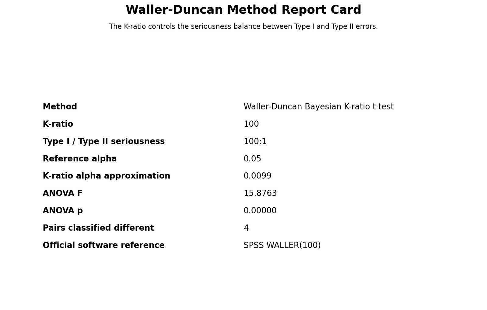
The method report card gives the main verification values for the Waller Duncan Test. It states that the analysis used the Waller-Duncan Bayesian K-ratio t test with K-ratio = 100. The Type I / Type II seriousness ratio is therefore 100:1. The chart also reports a reference alpha of 0.05 and a K-ratio alpha approximation of 0.0099.
The ANOVA line shows F = 15.8763 and p = 0.00000, which should be written as p < .001. The report card also states that 4 pairs were classified different. This makes the result easy to summarize: the omnibus ANOVA is significant, and the Waller-Duncan post hoc test separates some but not all group pairs.
Python Chart 2: Ordered Mean Intervals
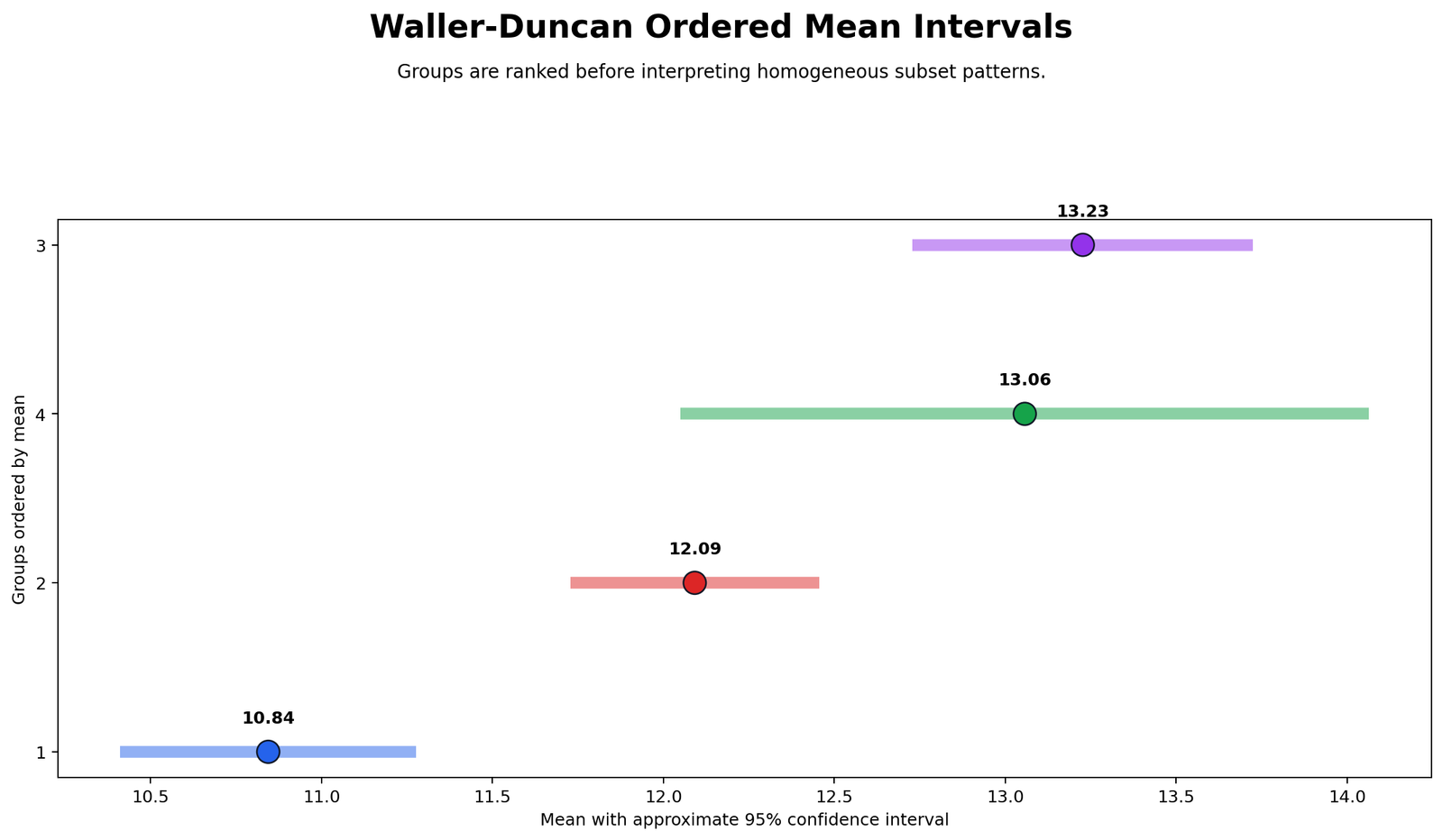
The ordered mean interval chart ranks the groups from lowest to highest. Group 1 has the lowest mean at 10.84. Group 2 follows at 12.09. Group 4 is higher at 13.06, and Group 3 has the highest mean at 13.23. This ranking provides the structure for the post hoc comparison because Waller-Duncan decisions are easier to read after the means are ordered.
The visual spacing shows why the final result contains both separation and overlap. The gap between Group 1 and the higher groups is large, so Group 1 is separated. The gap between Group 4 and Group 3 is very small, so those two are not separated. Group 4 also sits near enough to Group 2 to create the overlapping letter pattern AB.
Python Chart 3: K-Ratio Sensitivity
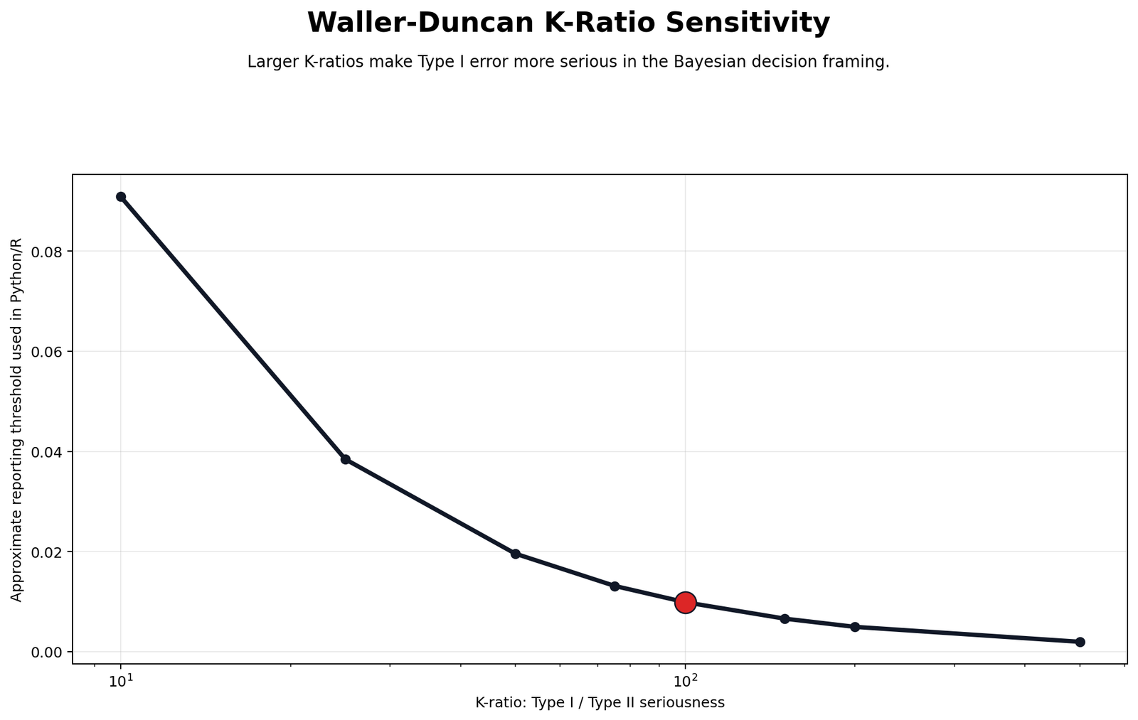
The K-ratio sensitivity chart shows the practical meaning of the Bayesian seriousness ratio. As the K-ratio increases, the approximate reporting threshold becomes smaller and the decision rule becomes more cautious about false positive differences. The highlighted point at K = 100 corresponds to an approximate threshold near 0.0099.
This chart is important because a Waller Duncan Test is not fully described unless the K-ratio is reported. Two researchers could use the same data but different K-ratios and obtain a different post hoc separation pattern. For this reason, the final report should write Waller-Duncan K-ratio t test, K = 100 rather than simply saying “Waller-Duncan post hoc test.”
Python Chart 4: Mean Difference vs Critical Difference
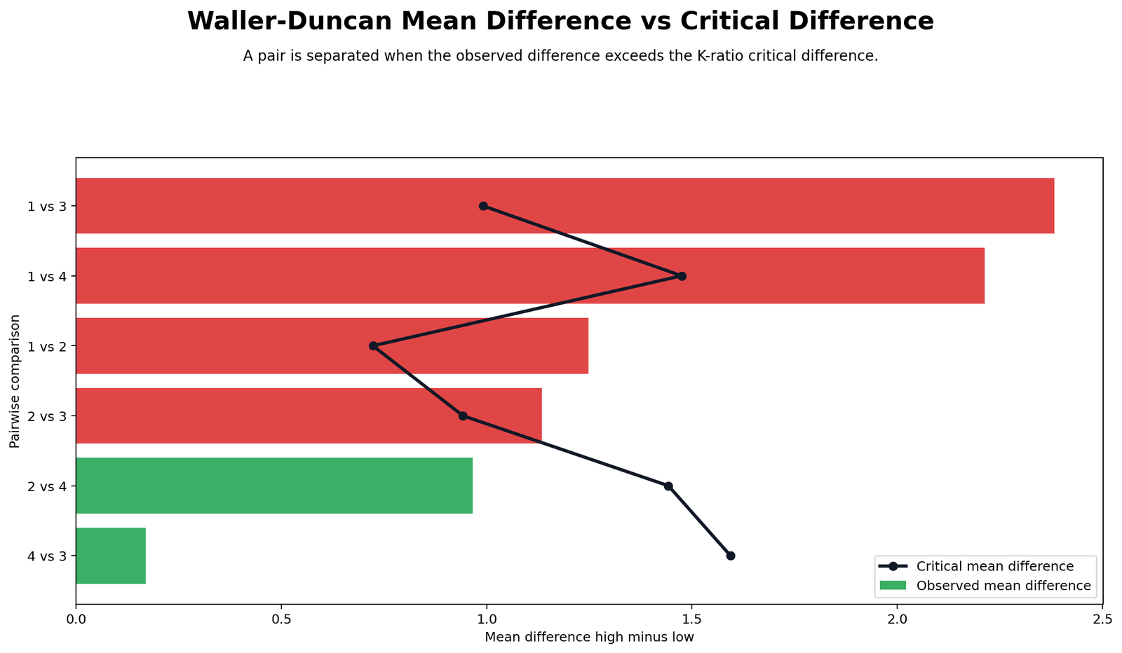
This chart compares each observed mean difference with its K-ratio critical difference. The red comparisons are separated because the observed difference exceeds the critical reference. The green comparisons are not separated because the observed mean difference is too small relative to the Waller-Duncan critical difference.
The chart shows that 1 vs 3, 1 vs 4, 1 vs 2, and 2 vs 3 are classified different. The comparisons 2 vs 4 and 4 vs 3 are not classified different. This is the core post hoc result and explains the final letter display: Group 1 stands alone at the bottom, Group 3 is in the highest group, and Group 4 bridges the higher and middle groups.
Python Chart 5: Pairwise t Statistics
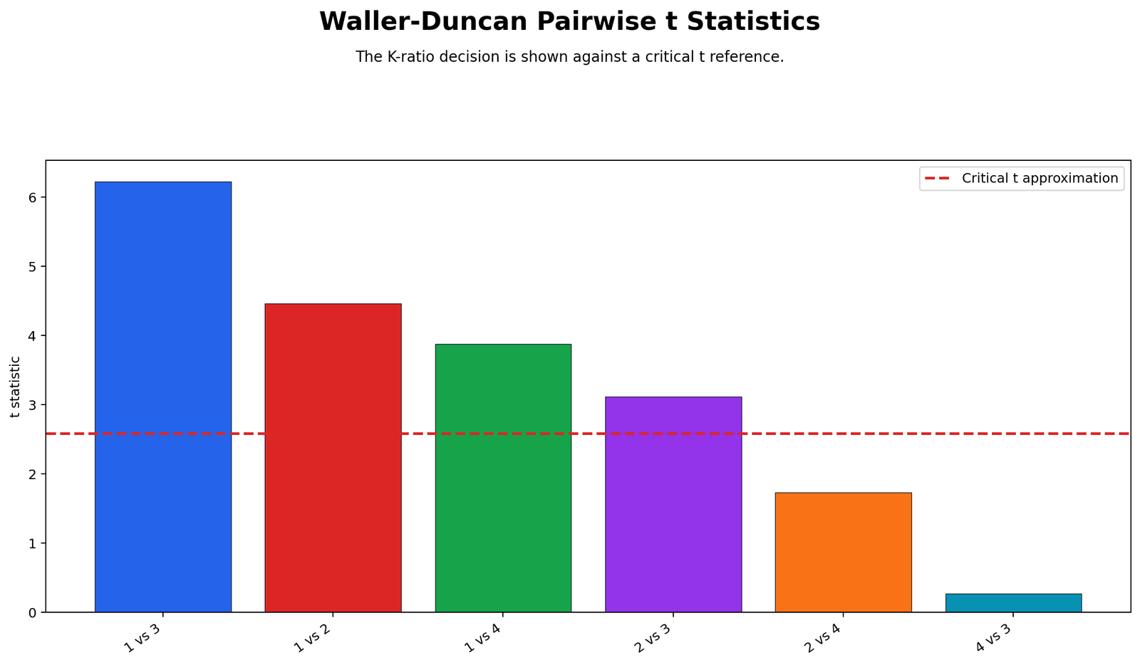
The t-statistics chart expresses the same pairwise comparisons on a standardized scale. The critical reference line is near the middle of the chart, and bars above that line are separated. The largest standardized separation is 1 vs 3, followed by 1 vs 2, 1 vs 4, and 2 vs 3. These are the four pairs classified different by the Waller-Duncan rule.
The smaller bars for 2 vs 4 and 4 vs 3 fall below the critical reference. This means those differences are not strong enough for separation under the K = 100 decision rule. The chart supports the same conclusion as the mean-difference chart but makes the comparison easier to read in t-statistic form.
Python Chart 6: Decision Matrix
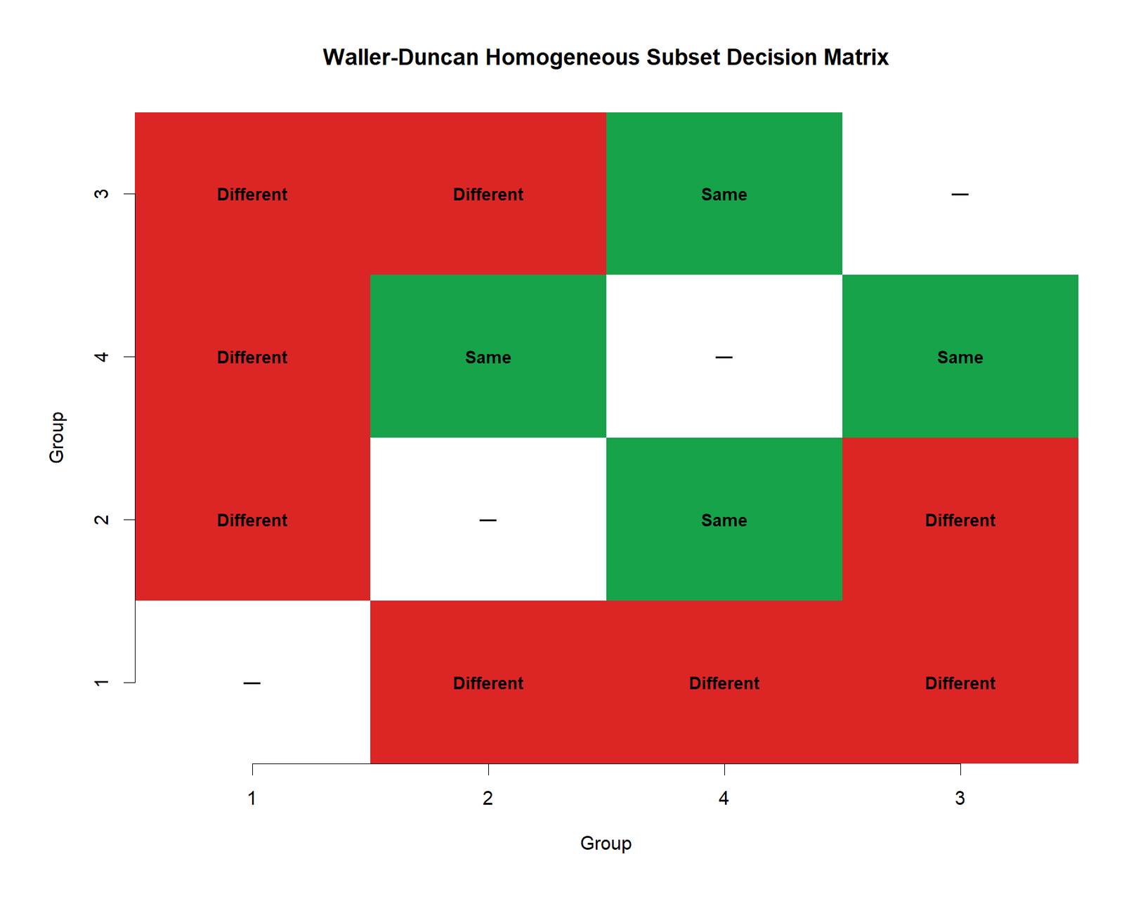
The decision matrix turns the pairwise result into a compact yes-or-no map. A separated cell means the two groups do not belong to the same homogeneous subset. A non-separated cell means the difference was not large enough under the Waller-Duncan K-ratio rule. This matrix is helpful because six pairwise comparisons can become difficult to follow in paragraph form.
The important reading is that Group 1 is separated from Groups 2, 4 and 3. Group 2 is separated from Group 3, but not from Group 4. Group 4 is not separated from Group 3. This is why the final grouping is not a simple four-level order. It is an overlapping pattern.
Python Chart 7: Homogeneous Subset Letters
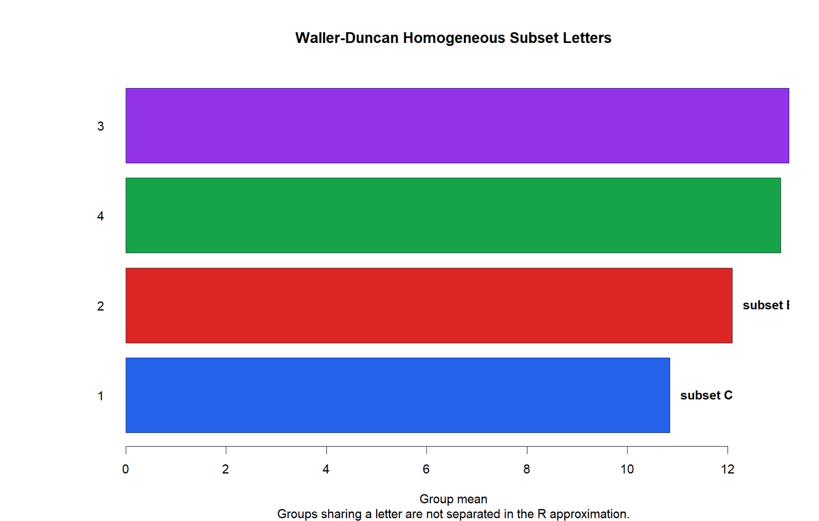
The homogeneous subset letter chart gives the most report-friendly version of the result. The expected compact letter display is Group 3 = A, Group 4 = AB, Group 2 = B, and Group 1 = C. Groups that share at least one letter are not separated. Groups that share no letter are separated.
This letter display communicates the overlapping middle pattern clearly. Group 4 shares A with Group 3 and B with Group 2. Therefore, Group 4 is not different from either Group 3 or Group 2, even though Group 3 and Group 2 are different from each other. Group 1 has C only, so it is separated from all higher groups.
Python Chart 8: Distribution Context
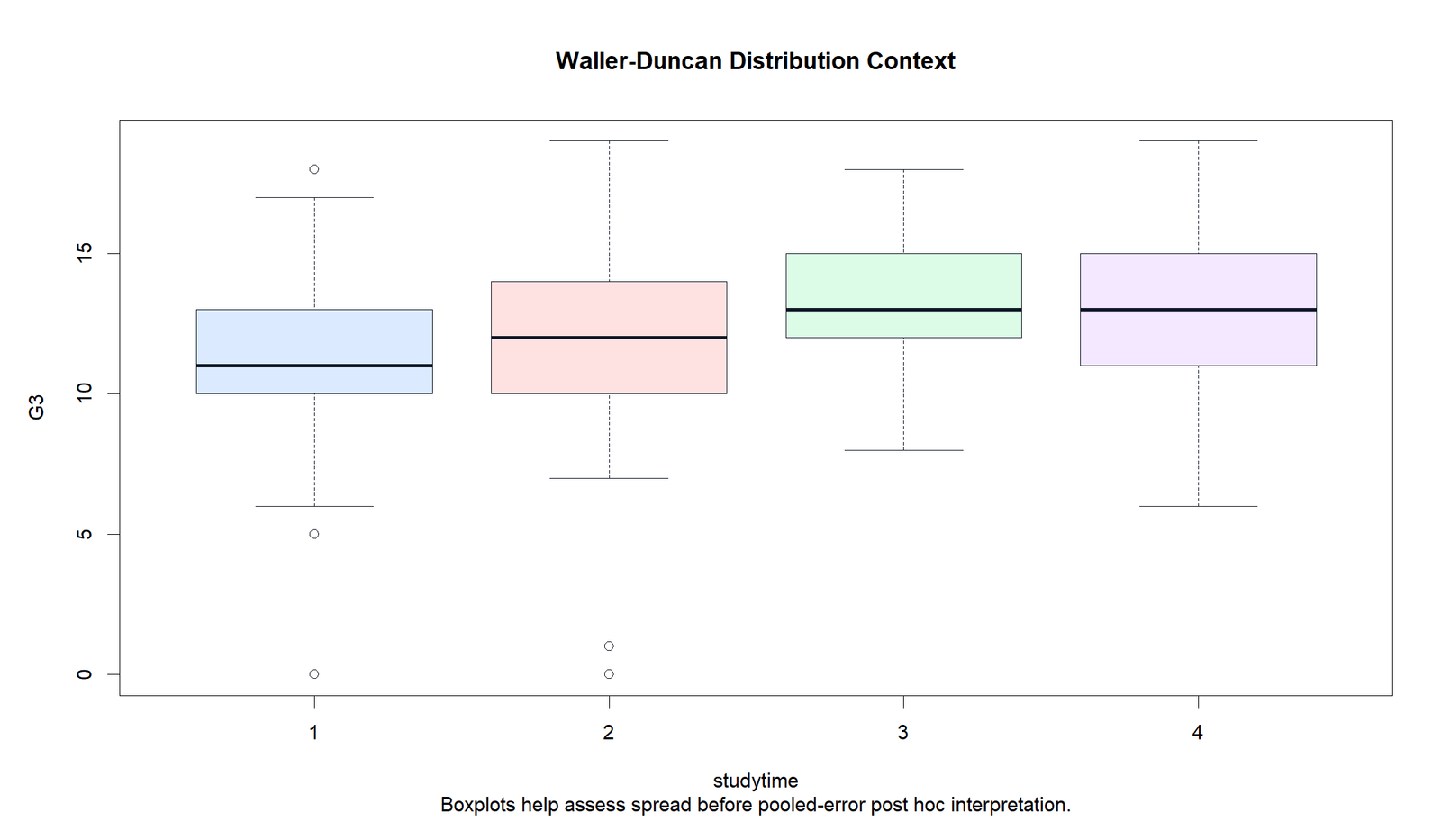
The distribution context chart adds practical meaning to the mean comparison. Post hoc tests compare means, but the researcher should still review the spread and overlap of the raw group distributions. A large mean gap with little distribution overlap usually supports stronger practical separation. A smaller mean gap with visible distribution overlap often explains why a pair is not classified different.
In this example, the distribution context supports the same interpretation as the ordered means and decision matrix. Group 1 is the low group. Group 3 and Group 4 are close at the top. Group 4 behaves as an overlapping bridge between the highest and middle levels. This helps prevent overreporting the result as four completely separate performance levels.
R Chart-by-Chart Validation
The R chart set validates the same Waller Duncan Test pattern using duplicated uploaded media filenames. The goal of R validation is to confirm that the conclusions are not dependent on one software workflow. The R charts should show the same method summary, ordered means, K-ratio sensitivity, pairwise decisions, t-statistics, decision matrix, subset letters and distribution context.
R Chart 1: Waller-Duncan Method Report Card
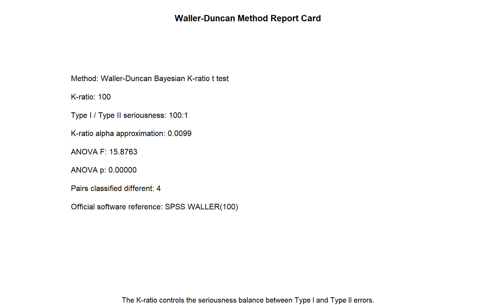
The R method report card should repeat the same key values: K = 100, reference alpha 0.05, K-ratio alpha approximation near 0.0099, significant ANOVA and 4 separated pairs. When R and SPSS agree on these values, confidence in the post hoc interpretation increases.
This chart is the quick validation checkpoint. Before reporting the details, confirm that the R method settings match the SPSS setting WALLER(100). If the K-ratio or alpha approximation differs, the pairwise result may not be directly comparable.
R Chart 2: Ordered Mean Intervals
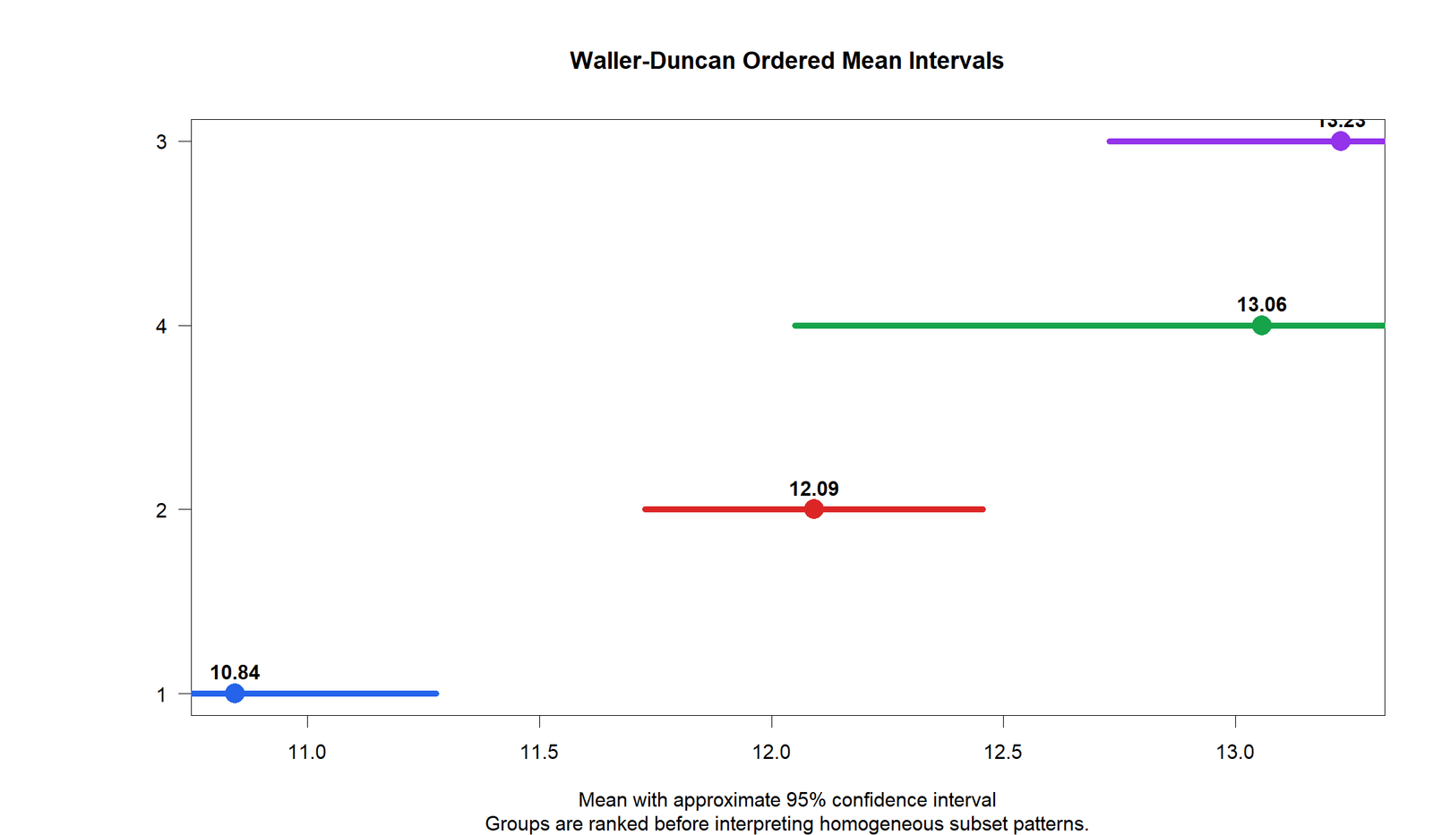
The R ordered mean chart should confirm the same ranking: Group 1 is lowest, Group 2 is second, Group 4 is third, and Group 3 is highest. This validates that the ordering is stable across workflows and that the same groups are being compared.
Because Waller-Duncan interpretation depends on ordered means, this validation step matters. If group labels or coding were accidentally changed in R, the ordered mean chart would reveal the problem before the final post hoc table is reported.
R Chart 3: K-Ratio Sensitivity
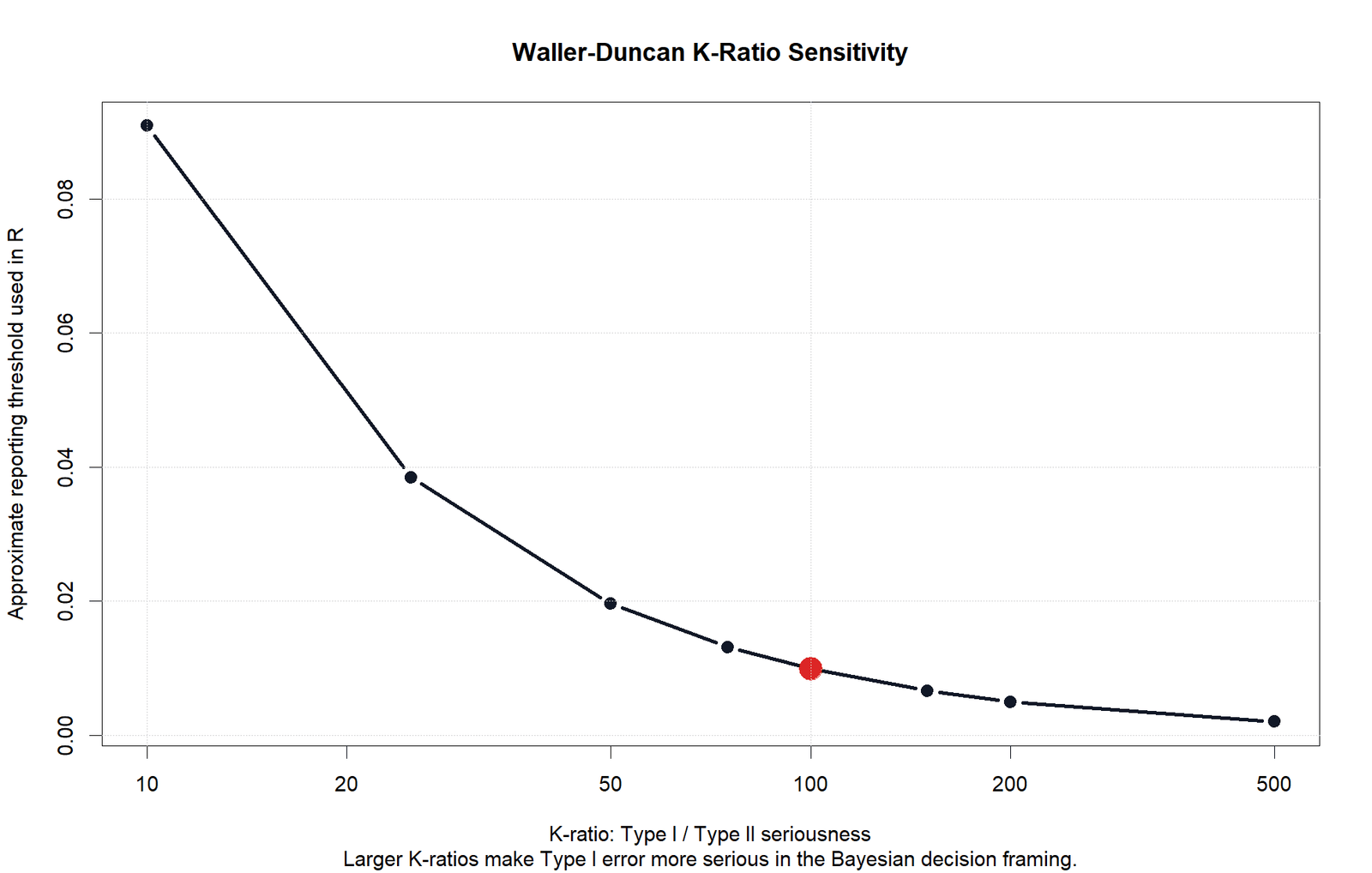
The R K-ratio sensitivity chart reinforces the same methodological point: K is not a decorative setting. It controls the seriousness balance between false positive and false negative decisions. A post hoc result reported without K is incomplete.
For this example, the selected K-ratio is 100. The validation chart should make clear that the comparison rule is stricter than a loose ordinary pairwise comparison, because the K-ratio alpha approximation is near 0.0099.
R Chart 4: Mean Difference vs Critical Difference
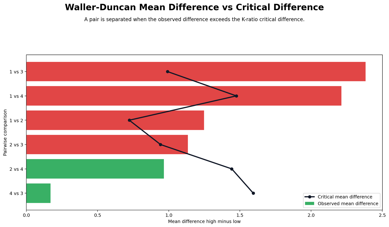
The R mean-difference chart should validate the same separated pairs as the Python chart. The separated comparisons are 1 vs 3, 1 vs 4, 1 vs 2, and 2 vs 3. The non-separated comparisons are 2 vs 4 and 4 vs 3.
This chart is especially useful because it shows the difference between a large numerical mean gap and a gap that is large enough for Waller-Duncan separation. Only gaps exceeding the critical reference are treated as statistically separated.
R Chart 5: Pairwise t Statistics
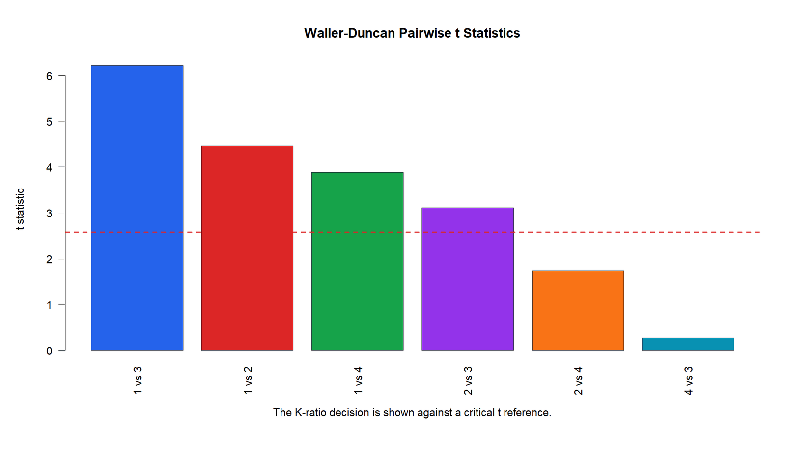
The R t-statistic chart should again show four comparisons above the critical reference and two below it. This validates the standardized version of the mean-difference result and confirms that the final decisions are not just visual impressions from the mean chart.
The strongest separation remains the comparison between the lowest and highest groups. The weakest comparison remains Group 4 versus Group 3, which is expected because their means are very close.
R Chart 6: Decision Matrix
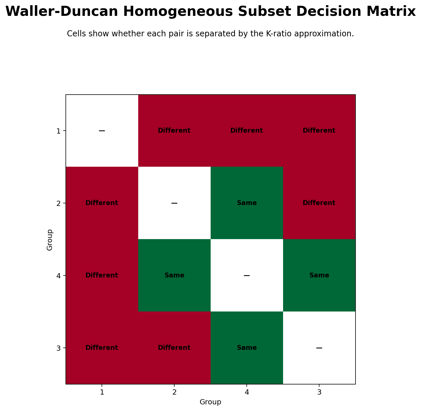
The R decision matrix should match the Python and SPSS decision pattern. A matching matrix confirms that the same four pairs are separated and the same two pairs remain non-separated. This is a strong check before writing the final interpretation.
The matrix format is useful for readers because it prevents confusion when subset letters overlap. The matrix explains why Group 4 can share a letter with Group 3 and also share a different letter with Group 2.
R Chart 7: Homogeneous Subset Letters
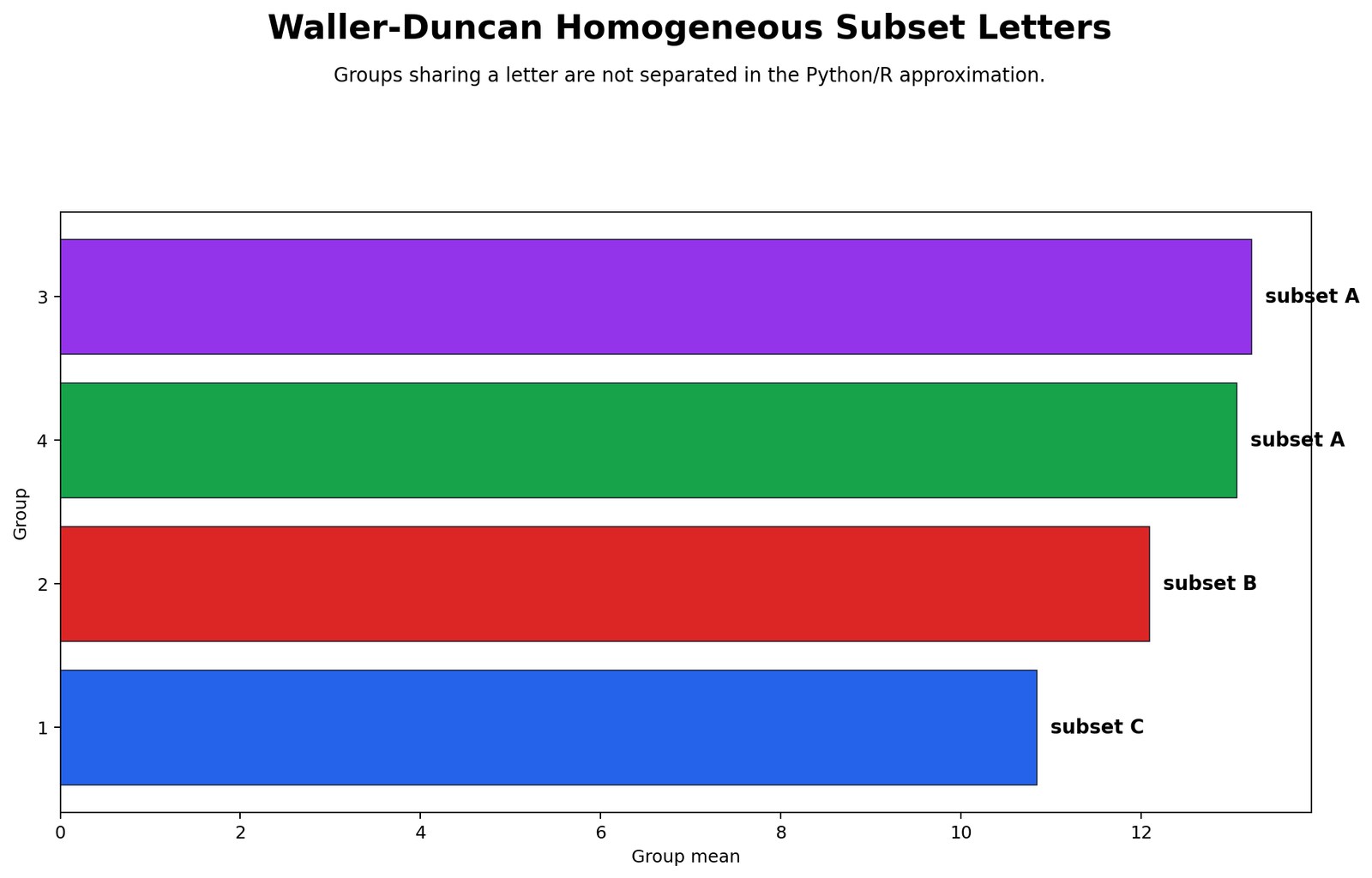
The R subset letter chart should confirm the compact display Group 3 = A, Group 4 = AB, Group 2 = B, and Group 1 = C. This is the easiest form to place in a results section because it gives both ranking and separation information.
The key interpretation is that groups sharing a letter are not separated. Group 4 shares A with Group 3 and B with Group 2. That overlap is the main reason the Waller-Duncan result should not be described as four completely separate groups.
R Chart 8: Distribution Context
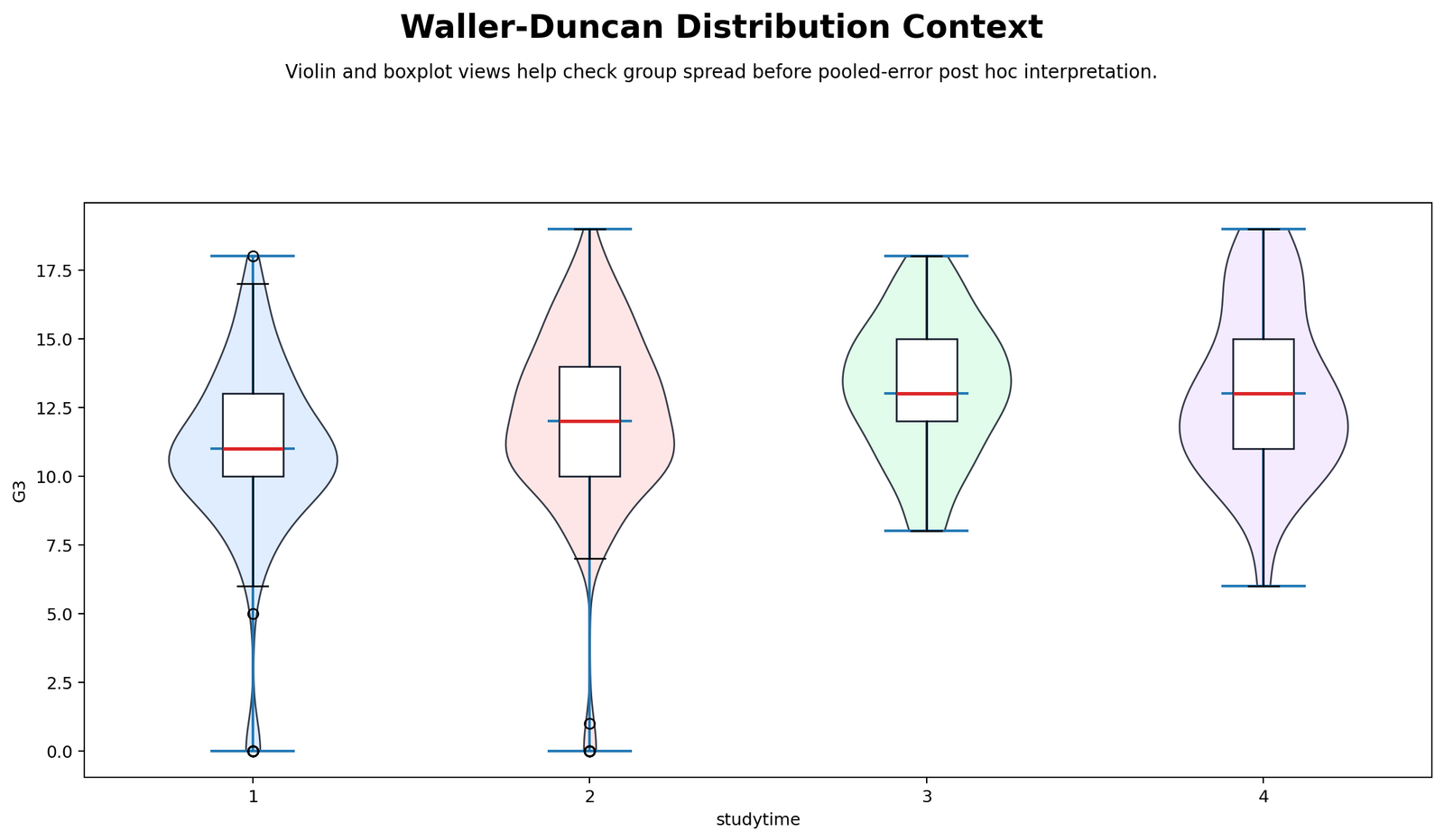
The R distribution context chart supports the final interpretation by showing the spread behind the group means. Post hoc tests are based on mean comparisons, but distribution context helps readers understand whether the result is practically meaningful and visually reasonable.
The main message remains consistent: Group 1 is the lower group, Group 3 and Group 4 are high and close, and Group 4 functions as an overlapping bridge between the high and middle subsets.
SPSS, R, Python and Excel Workflows for Waller Duncan Test
The Waller Duncan Test can be approached in SPSS, R, Python and Excel. SPSS is the most direct option because it includes the WALLER(K) post hoc reference. R can reproduce Waller-Duncan using specialized post hoc tools or custom calculations. Python can build the decision report from ANOVA MSE, group means and a K-ratio threshold approximation. Excel is best for learning and transparent manual checking.
SPSS Workflow
| Step | SPSS Action | Purpose |
|---|---|---|
| Open dataset | File > Open > Data | Load the clean dataset with one numeric dependent variable and one grouping factor. |
| Run ANOVA | Analyze > Compare Means > One-Way ANOVA | Test whether the group means differ overall. |
| Select post hoc | Post Hoc > Waller-Duncan | Request the Waller-Duncan K-ratio post hoc test. |
| Set K-ratio | Use K = 100 | Match the seriousness ratio used in this report. |
| Review output | Read homogeneous subsets and pairwise decisions | Identify which groups are separated and which groups overlap. |
| Export report | File > Export or OUTPUT EXPORT | Save the SPSS output PDF for verification. |
R Workflow
| Step | R Action | Purpose |
|---|---|---|
| Read data | read.csv() | Load the dataset into R. |
| Fit ANOVA | aov(score ~ group, data = data) | Estimate group mean differences and MSE. |
| Run Waller-Duncan | agricolae::waller.test() or custom function | Produce K-ratio group separation. |
| Order means | Sort group means from low to high | Prepare the homogeneous subset display. |
| Create charts | ggplot2 | Visualize ordered means, pairwise decisions and subset letters. |
| Export results | ggsave() and PDF output | Create reproducible files for the article. |
Python Workflow
| Step | Python Action | Purpose |
|---|---|---|
| Read data | pandas.read_csv() | Load the dataset. |
| Fit ANOVA | statsmodels.formula.api.ols() | Estimate the one-way ANOVA model. |
| Extract MSE | Use residual mean square from ANOVA table | Calculate pairwise standard errors. |
| Apply K-ratio threshold | Use K = 100 approximation or validated rule | Classify pairwise differences. |
| Build decision matrix | Create pairwise decision table | Summarize which pairs are separated. |
| Plot charts | matplotlib | Create report card, ordered means, t statistics and subset charts. |
Excel Workflow
| Step | Excel Action | Purpose |
|---|---|---|
| Prepare columns | One column for score and one column for group | Keep the data in long format. |
| Calculate group means | AVERAGEIF() | Find the mean for each group. |
| Calculate group counts | COUNTIF() | Find sample size for each group. |
| Get ANOVA MSE | Data Analysis ToolPak ANOVA | Use the within-group mean square error. |
| Pairwise differences | ABS(mean_i - mean_j) | Calculate observed differences. |
| Approximate decision | Compare difference with a K-ratio critical reference | Create an educational Waller-Duncan style decision table. |
Code Blocks for Waller Duncan Test
The following code blocks show how the analysis can be organized in SPSS, R, Python and Excel. For exact SPSS-style reporting, the SPSS WALLER(100) output should be treated as the reference result.
SPSS Syntax
* Waller Duncan Test in SPSS.
* Replace score and group with your actual variable names.

ONEWAY score BY group
  /STATISTICS DESCRIPTIVES HOMOGENEITY
  /MISSING ANALYSIS
  /POSTHOC = WALLER(100) ALPHA(0.05).

OUTPUT EXPORT
  /CONTENTS EXPORT=VISIBLE
  /PDF DOCUMENTFILE='Waller-Duncan-Test-SPSS-Output.pdf'.
R Code
# Waller Duncan Test in R
# Install packages if needed:
# install.packages(c("agricolae", "ggplot2", "dplyr"))

library(agricolae)
library(ggplot2)
library(dplyr)

data <- read.csv("dataset.csv")

# Make sure group is treated as a factor
data$group <- as.factor(data$group)

# One-way ANOVA
model <- aov(score ~ group, data = data)
summary(model)

# Waller-Duncan K-ratio test
wd <- waller.test(model, "group", K = 100, alpha = 0.05, group = TRUE)
print(wd)

# Ordered means
means <- data %>%
  group_by(group) %>%
  summarise(
    n = n(),
    mean = mean(score, na.rm = TRUE),
    sd = sd(score, na.rm = TRUE),
    .groups = "drop"
  ) %>%
  arrange(mean)

print(means)
Python Code
# Waller Duncan style workflow in Python
# This builds ANOVA, ordered means, and pairwise decision support.
# Validate exact Waller-Duncan decisions against SPSS WALLER(100)
# when official reporting is required.

import itertools
import numpy as np
import pandas as pd
import scipy.stats as stats
import statsmodels.api as sm
import statsmodels.formula.api as smf
from statsmodels.stats.anova import anova_lm

data = pd.read_csv("dataset.csv")
data["group"] = data["group"].astype("category")

# One-way ANOVA
model = smf.ols("score ~ C(group)", data=data).fit()
anova = anova_lm(model, typ=2)
print(anova)

mse = anova.loc["Residual", "sum_sq"] / anova.loc["Residual", "df"]
df_error = anova.loc["Residual", "df"]

summary = (
    data.groupby("group")["score"]
    .agg(["count", "mean", "std"])
    .reset_index()
    .sort_values("mean")
)

print(summary)

# K-ratio approximation used for educational reporting support
K = 100
alpha_k = 1 / (K + 1)
tcrit = stats.t.ppf(1 - alpha_k / 2, df_error)

rows = []
for g1, g2 in itertools.combinations(summary["group"], 2):
    x1 = data.loc[data["group"] == g1, "score"].dropna()
    x2 = data.loc[data["group"] == g2, "score"].dropna()
    mean_diff = abs(x1.mean() - x2.mean())
    se = np.sqrt(mse * (1 / len(x1) + 1 / len(x2)))
    t_stat = mean_diff / se
    decision = "Different" if t_stat > tcrit else "Not different"
    rows.append([g1, g2, mean_diff, se, t_stat, tcrit, decision])

pairwise = pd.DataFrame(
    rows,
    columns=["Group 1", "Group 2", "Mean Difference", "SE", "t", "Critical t", "Decision"]
)

print(pairwise)
Excel Formula Guide
Assume:
A:A = group
B:B = score

Group mean:
=AVERAGEIF($A:$A, D2, $B:$B)

Group count:
=COUNTIF($A:$A, D2)

Observed pairwise difference:
=ABS(mean_i - mean_j)

Pairwise standard error:
=SQRT(MSE * (1/n_i + 1/n_j))

Approximate t statistic:
=Observed_Difference / Standard_Error

K-ratio alpha approximation for K = 100:
=1/(100+1)

Approximate two-tailed critical t:
=T.INV.2T(1/(100+1), df_error)

Decision:
=IF(t_stat > critical_t, "Different", "Not different")
APA Reporting Wording for Waller Duncan Test
When reporting the Waller Duncan Test, include the omnibus ANOVA result, the K-ratio, the pairwise pattern and the homogeneous subset letters. Do not report the printed value p = 0.00000 as a literal zero. Use p < .001.
APA-style example: A one-way ANOVA showed a statistically significant difference among the four group means, F = 15.8763, p < .001. Waller-Duncan Bayesian K-ratio post hoc comparisons were conducted using K = 100. The test classified four of six pairwise comparisons as different. Group 1 had the lowest mean (M = 10.84) and was separated from Groups 2, 4 and 3. Group 3 had the highest mean (M = 13.23) and was separated from Groups 2 and 1, but not from Group 4. A compact letter display summarized the pattern as Group 3 = A, Group 4 = AB, Group 2 = B and Group 1 = C.
| Report Element | Recommended Wording | Why It Matters |
|---|---|---|
| Omnibus result | F = 15.8763, p < .001 | Shows that post hoc testing is justified. |
| Post hoc method | Waller-Duncan Bayesian K-ratio t test | Names the exact comparison procedure. |
| K-ratio | K = 100 | Defines the Type I / Type II seriousness balance. |
| Pairwise result | 4 of 6 pairs were classified different | Summarizes the post hoc outcome. |
| Letters | 3 = A, 4 = AB, 2 = B, 1 = C | Communicates homogeneous subset overlap clearly. |
Common Mistakes in Waller Duncan Test
The most common mistake is reporting the Waller Duncan Test without the K-ratio. The K-ratio is not optional decoration. It is part of the definition of the decision rule. A result reported as “Waller-Duncan post hoc test was significant” is incomplete unless the K-ratio and pairwise pattern are also reported.
Another mistake is treating homogeneous subset letters as pure ranking labels. Letters are not ordinary ranks. Groups sharing a letter are not separated. In this example, Group 4 has AB, meaning it overlaps with both the A group and the B group. This does not mean Group 4 is both first and second in a simple rank order. It means the pairwise decisions place it between the high and middle subsets.
| Mistake | Why It Is Wrong | Correct Approach |
|---|---|---|
| Ignoring the ANOVA stage | Post hoc tests are follow-up procedures. | Report the ANOVA first. |
| Not reporting K | The decision rule depends on K. | Write Waller-Duncan K = 100. |
| Writing p = 0.000 | A p-value is not literally zero. | Write p < .001. |
| Calling all means different | Only 4 of 6 pairs were separated. | Report the exact pairwise pattern. |
| Misreading AB | AB means overlap, not a fixed rank. | Explain shared letters as non-separated groups. |
| Using it when variances are badly unequal | Classical ANOVA post hoc methods assume suitable ANOVA conditions. | Check Levene’s test and consider robust alternatives. |
When to Use Waller Duncan Test
Use the Waller Duncan Test when you have a significant ANOVA and you want a post hoc procedure that explicitly balances Type I and Type II error seriousness through a K-ratio. It is especially useful when the reporting goal is to form homogeneous subsets and explain which ordered means are separated.
The test is less appropriate when the main priority is very strict familywise error control, when variances are strongly unequal, or when sample sizes and assumptions make classical ANOVA post hoc comparisons questionable. In those cases, consider checking ANOVA assumptions, Levene’s test, Brown-Forsythe ANOVA, or Welch-type alternatives.
| Use Waller Duncan Test When | Be Careful When |
|---|---|
| You have a significant one-way ANOVA. | The ANOVA is not significant and no planned comparison exists. |
| You want homogeneous subset letters. | You only need a single planned contrast. |
| You can justify a K-ratio such as K = 100. | You cannot explain why that K-ratio was selected. |
| Group variances and assumptions are acceptable. | Variance heterogeneity is severe. |
| You want to compare ordered group means. | You need a nonparametric or robust post hoc method. |
Downloads and Resources
Use the resources below to verify the Waller Duncan Test workflow and reproduce the chart-based interpretation. These files support the SPSS, Python and R explanations in this guide.
FAQs About Waller Duncan Test
What is the Waller Duncan Test?
The Waller Duncan Test is a post hoc ANOVA comparison method that uses a Bayesian K-ratio to decide which group means are significantly separated after an omnibus ANOVA.
What does K = 100 mean in Waller Duncan Test?
K = 100 means the method treats a Type I error as 100 times as serious as a Type II error. The K-ratio affects the critical threshold and should always be reported.
How do I report SPSS WALLER(100)?
Report the ANOVA result first, then write that Waller-Duncan Bayesian K-ratio post hoc comparisons were conducted using K = 100. Include the separated pairs or compact letter display.
What does AB mean in homogeneous subset letters?
AB means the group overlaps with both the A subset and the B subset. It is not separated from groups sharing A and not separated from groups sharing B.
Is Waller Duncan the same as Tukey test?
No. Tukey-style methods focus on multiple comparison error control in a different way. The Waller Duncan Test uses a K-ratio seriousness balance between Type I and Type II errors.
Can I do Waller Duncan Test in Excel?
Excel can approximate the learning workflow by calculating group means, ANOVA MSE, pairwise standard errors and t decisions. For exact official reporting, SPSS WALLER(100) or a validated R/Python implementation should be used.

