
One-Sample Mean Test, Two Rejection Regions, P Value, Critical Value and Confidence Interval
Two Tailed T Test: Formula, P Value, Critical Value, SPSS, Python, R and Excel Guide
Two Tailed T Test is used when a researcher wants to know whether a sample mean is significantly different from a hypothesized value in either direction. It is called two tailed because the rejection area is split into the left tail and right tail of the t distribution. This guide explains the two tailed t test formula, two tailed t test p value, two tailed t test critical value, two tailed rejection regions, one tailed vs two tailed t test, SPSS output interpretation, Python chart interpretation, R validation charts, Excel workflow, APA reporting, common mistakes and downloadable resources using G3 final grade from the student performance dataset.
Quick Answer: Two Tailed T Test Result
The worked example tests whether the mean G3 final grade is significantly different from the null mean of 10. The sample contains 649 students. The sample mean is approximately 11.906, the mean difference is approximately 1.906, and the two-tailed result is statistically significant with t(648) = 15.03, p < .001.
The 95% confidence interval for the mean is approximately 11.657 to 12.155. Because this interval is completely above the null mean of 10, the confidence interval agrees with the two-tailed p-value decision. The result shows that the mean G3 score is not equal to 10; it is significantly higher than 10 in this dataset.
Final interpretation: The two tailed t test rejects the null hypothesis. The mean G3 score is significantly different from 10, and the observed direction is higher because the sample mean is above the null mean.
Important reporting point: A two tailed t test does not test only “greater than” or only “less than.” It tests for difference in either direction. Even if the observed result is higher, the hypothesis remains two tailed when the alternative is μ ≠ μ0.
Table of Contents
- What Is a Two Tailed T Test?
- Two Tailed T Test Formula
- Null and Alternative Hypothesis
- Dataset and Variables Used
- SPSS Output Interpretation
- Python Chart-by-Chart Interpretation
- R Chart-by-Chart Validation
- SPSS, R, Python and Excel Workflows
- Code Blocks for Two Tailed T Test
- APA Reporting Wording
- Common Mistakes
- When to Use Two Tailed T Test
- Downloads and Resources
- Related Guides
- FAQs
What Is a Two Tailed T Test?
A Two Tailed T Test is a hypothesis test used to decide whether a sample mean is significantly different from a hypothesized population mean. It is called “two tailed” because the test allows evidence in both directions. If the sample mean is much lower than the null mean, the result can fall in the left rejection region. If the sample mean is much higher than the null mean, the result can fall in the right rejection region.
In a two tailed test, the alternative hypothesis uses the “not equal to” symbol. This makes it different from a one tailed t test. A one tailed test checks only one direction, such as greater than or less than. A two tailed t test is more conservative when the direction is not known in advance because alpha is divided between two tails.
The most common two tailed one-sample t test asks whether the sample mean differs from a fixed value. In this guide, the sample mean of G3 final grade is compared with the null mean of 10. The test result is significant because the sample mean is far enough above the null mean that the two-tailed p value is below .05.
Simple definition: A two tailed t test checks whether a mean is significantly different from a null value, allowing the difference to be either lower or higher.
This guide is connected with other t-test and assumption guides, including One Tailed T Test, One Sample T Test, T Test Assumptions, P Value, Confidence Interval, Effect Size, Standard Error, Q-Q Plot Normality Check, and Histogram Interpretation.
Two Tailed T Test Formula
The one-sample Two Tailed T Test uses the same t statistic formula as a one-sample t test. The tail direction changes the hypothesis and p-value interpretation, not the basic t statistic calculation.
In this formula, x̄ is the sample mean, μ0 is the null mean, s is the sample standard deviation, and n is the sample size. The denominator s / √n is the standard error of the mean.
Two Tailed P Value Formula
The two tailed p value is calculated by taking the probability of a t statistic at least as extreme as the observed absolute value and doubling it:
Two Tailed Critical Value Rule
For a two tailed test at alpha = .05, the rejection area is split into two tails. Each tail receives .025 of the total alpha.
| Formula Component | Meaning | Worked Example Value |
|---|---|---|
| x̄ | Sample mean | 11.906 |
| μ0 | Null mean | 10.000 |
| x̄ − μ0 | Mean difference | 1.906 |
| n | Sample size | 649 |
| df | Degrees of freedom | 648 |
| t | Test statistic | 15.03 |
| p | Two-tailed p value | < .001 |
Threshold rule: If the two-tailed p value is less than alpha, reject the null hypothesis. At alpha = .05, a p value below .05 means the sample mean is significantly different from the null mean in either direction.
Null and Alternative Hypothesis
A Two Tailed T Test uses a non-directional alternative hypothesis. The test asks whether the mean is different from the null mean, not specifically greater than or less than the null mean.
| Statement | Symbolic Form | Meaning for This Example |
|---|---|---|
| Null hypothesis | H0: μ = 10 | The population mean G3 score equals 10. |
| Alternative hypothesis | H1: μ ≠ 10 | The population mean G3 score is different from 10. |
| Decision rule | Reject H0 if p < .05 | The mean is significantly different from 10. |
Decision for this example: The null hypothesis is rejected because p < .001. The sample mean is significantly different from 10. The observed direction is higher because the sample mean is 11.906.
Dataset and Variables Used
The worked example uses a student performance dataset with 649 valid cases. The formal two tailed t test uses G3 final grade as the numeric test variable and compares its mean against the null value 10. Additional context charts use school and studytime to explain how G3 varies across groups, but the main hypothesis test is a one-sample two tailed t test.
| Variable or Value | Role | Why It Matters |
|---|---|---|
| G3 | Test variable | The final grade variable whose mean is tested. |
| 10 | Null mean | The hypothesized mean used for comparison. |
| school | Context variable | Shows whether G3 differs descriptively by school group. |
| studytime | Context variable | Shows whether G3 differs descriptively by study-time category. |
| 649 | Sample size | Determines degrees of freedom and standard error. |
Before interpreting a two tailed t test, it is helpful to inspect descriptive statistics, histograms, confidence intervals, and the normality pattern. Related resources include Descriptive Statistics, Histogram Interpretation, Standard Deviation, and Standard Error.
SPSS Output Interpretation for Two Tailed T Test
In SPSS, the two tailed one-sample t test is run through Analyze > Compare Means > One-Sample T Test. The variable G3 is placed in the Test Variable(s) box, and the test value is set to 10. SPSS reports the result as Sig. (2-tailed), which is the two-tailed p value.
SPSS Output Values to Read
| SPSS Output Item | Value or Meaning | Interpretation |
|---|---|---|
| Test Variable | G3 | Final grade is the numeric outcome being tested. |
| Test Value | 10 | The null mean used in the one-sample t test. |
| Mean | 11.906 | The observed sample mean is higher than the null mean. |
| Mean Difference | 1.906 | The sample mean is about 1.906 points above 10. |
| t | 15.03 | The observed difference is large relative to the standard error. |
| df | 648 | Degrees of freedom equal n − 1. |
| Sig. (2-tailed) | < .001 | The two-tailed p value is statistically significant. |
SPSS Chart 1: G3 Distribution with Null and Sample Mean
This SPSS chart shows the distribution of G3 values and marks both the null mean and the sample mean. The sample mean appears above the null mean, which visually explains why the t statistic is positive.
The chart supports the statistical result because the mean is not only above the null value but far enough away that the two-tailed p value is below .001.
SPSS Chart 2: Null Mean vs Sample Mean
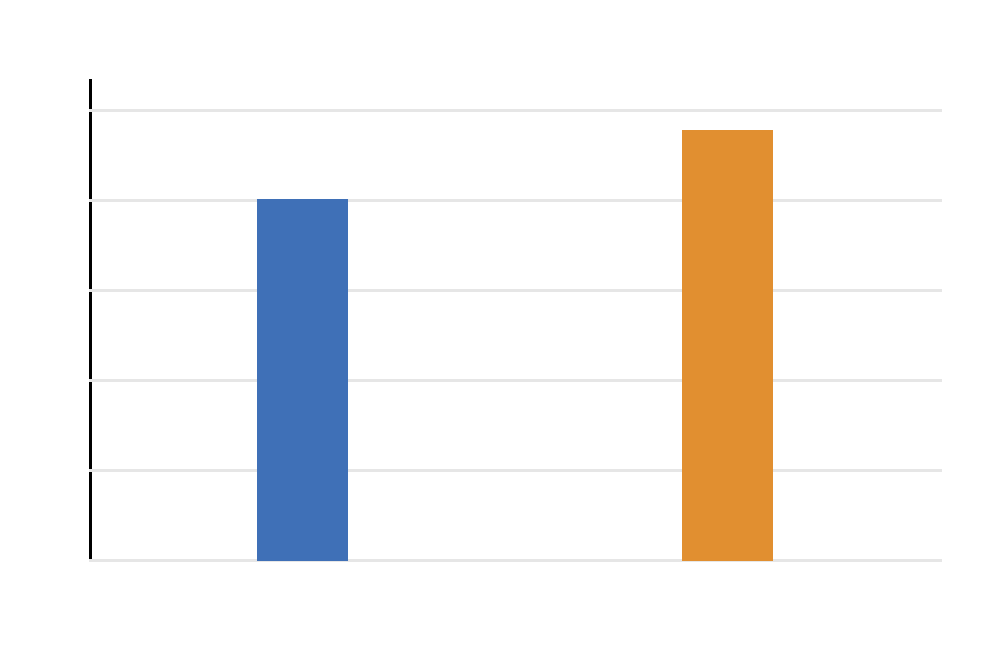
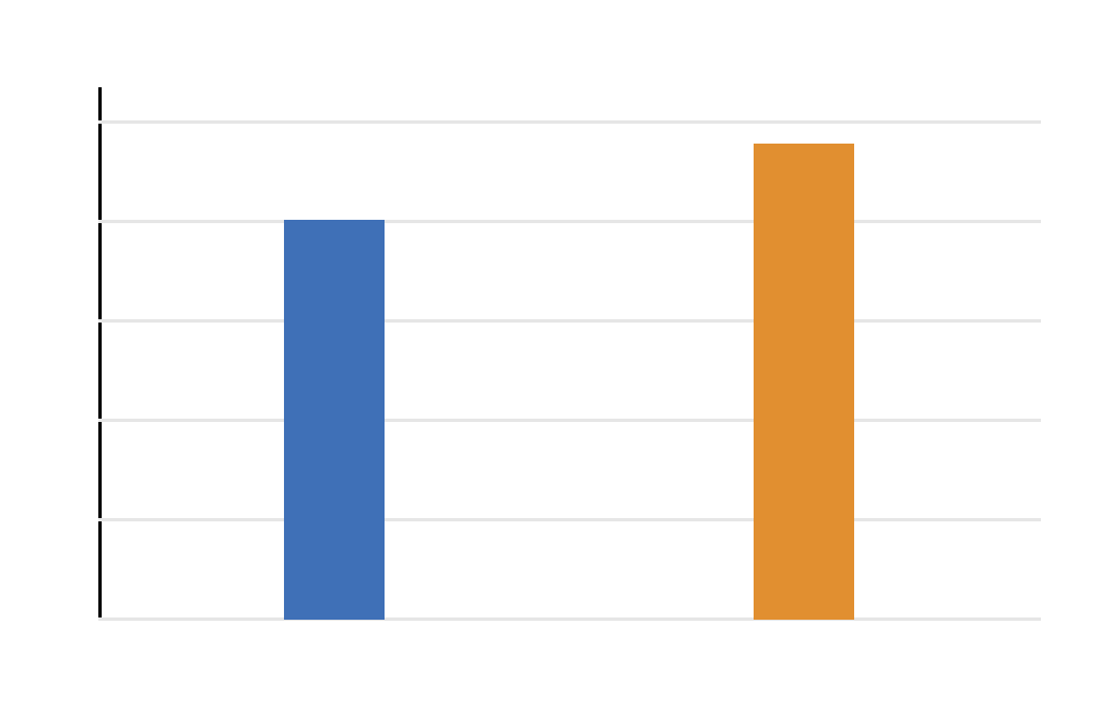
This chart focuses directly on the comparison between the null mean of 10 and the sample mean of about 11.906. The difference is positive because the sample mean is higher.
In a two tailed test, the direction is interpreted after the test. The hypothesis was non-directional, but the observed result is higher than the null value.
SPSS Chart 3: Mean Confidence Interval
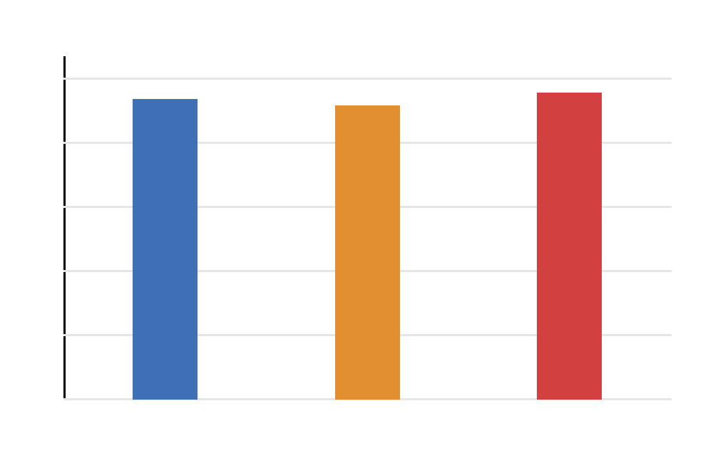
The confidence interval chart shows the plausible range for the population mean. The interval is above 10, which agrees with the hypothesis test decision.
This chart is useful because confidence intervals explain both statistical significance and practical location of the mean.
SPSS Chart 4: T Statistic Distribution Curve
This chart shows the observed t statistic on the t distribution. Because this is a two tailed t test, the rejection region is split into the left and right tails.
The observed statistic is positive and far into the right side, so the null hypothesis is rejected.
SPSS Chart 5: Mean Difference Confidence Interval
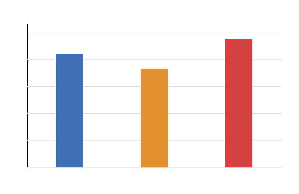
This chart shows the confidence interval for the difference between the sample mean and the null mean. The interval is above zero, which means the mean difference is significantly positive.
Because the difference interval does not cross zero, the two-tailed null hypothesis is rejected.
SPSS Chart 6: Mean G3 by School Context
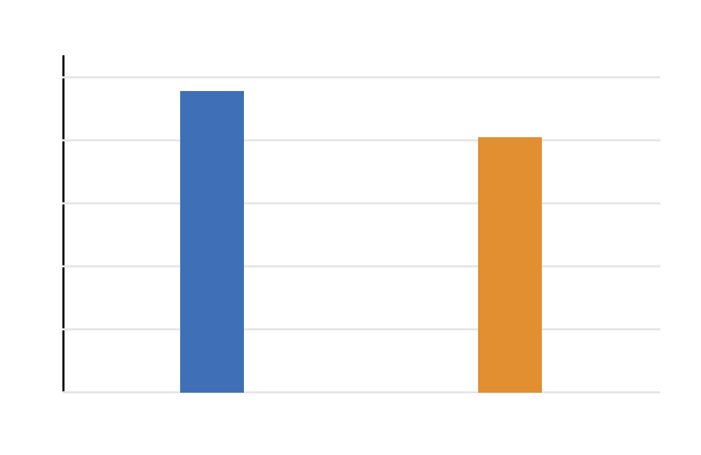
This chart adds school-level context for the G3 variable. It is not the main hypothesis test, but it helps explain the outcome variable across school groups.
The formal two tailed t test remains the comparison between overall mean G3 and the null mean of 10.
SPSS Chart 7: Mean G3 by Studytime Context
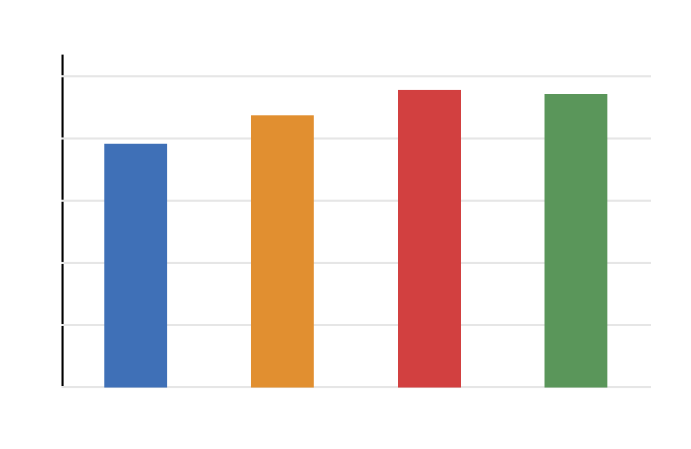
This chart shows how mean G3 varies across studytime categories. It gives descriptive background for the outcome variable.
Context charts are useful for explanation but should not be confused with the formal one-sample two tailed t test.
SPSS Chart 8: Two Tailed T Test Main Result Table
This is the main SPSS results table. It reports t, degrees of freedom, Sig. (2-tailed), mean difference and confidence interval information.
The key value is Sig. (2-tailed). Since it is below .05, the test rejects the null hypothesis.
SPSS Chart 9: Tail Decision Table
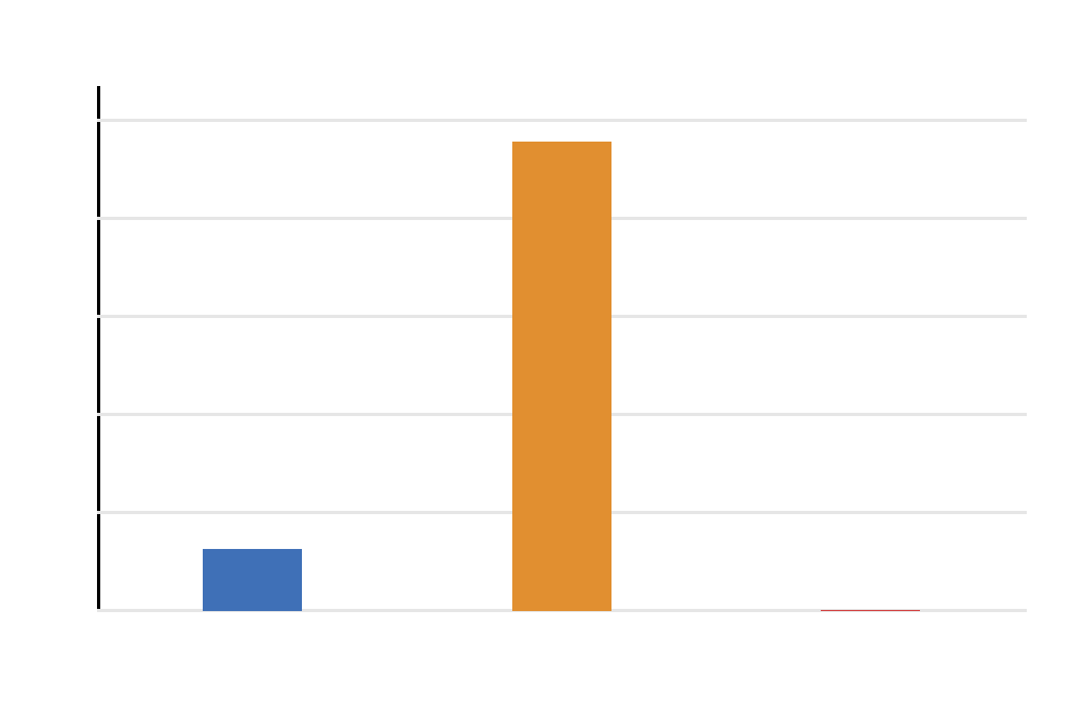
This decision table explains how to read a two-tailed result. If the two-tailed p value is less than alpha, reject H0. If the confidence interval excludes the null mean, the same conclusion is supported.
For this example, both the p value and confidence interval support rejection of the null hypothesis.
SPSS Chart 10: School Context Table
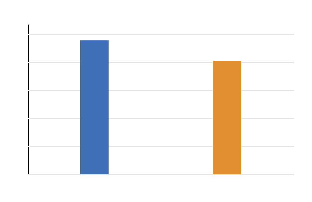
This table summarizes G3 by school group. It supports descriptive interpretation and helps readers understand variation in the dataset.
The school context table is supplementary; the formal result is still the two-tailed one-sample t test of G3 against 10.
Python Chart-by-Chart Interpretation
The Python charts show the same Two Tailed T Test workflow visually. They include the G3 distribution, null mean versus sample mean, confidence interval, two rejection regions, mean difference, context charts, descriptives table, results table and tail decision table.
Python Chart 1: G3 Distribution with Null Mean
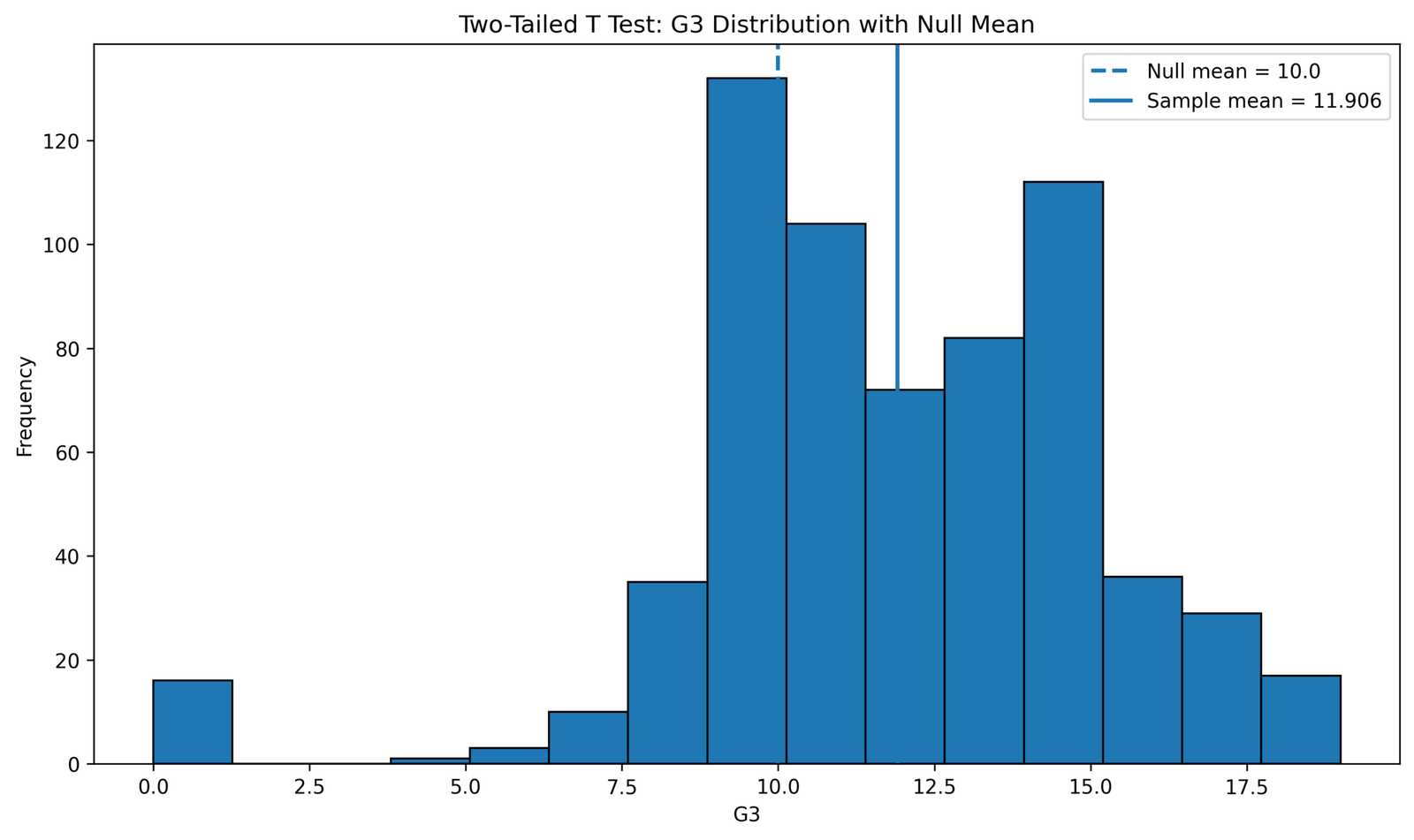
This chart shows the distribution of G3 scores and marks the null mean. The sample mean is positioned above the null mean, which explains the positive t statistic.
The chart supports the final conclusion because the sample mean is not only higher but statistically far from the null value when standard error is considered.
Python Chart 2: Null Mean vs Sample Mean
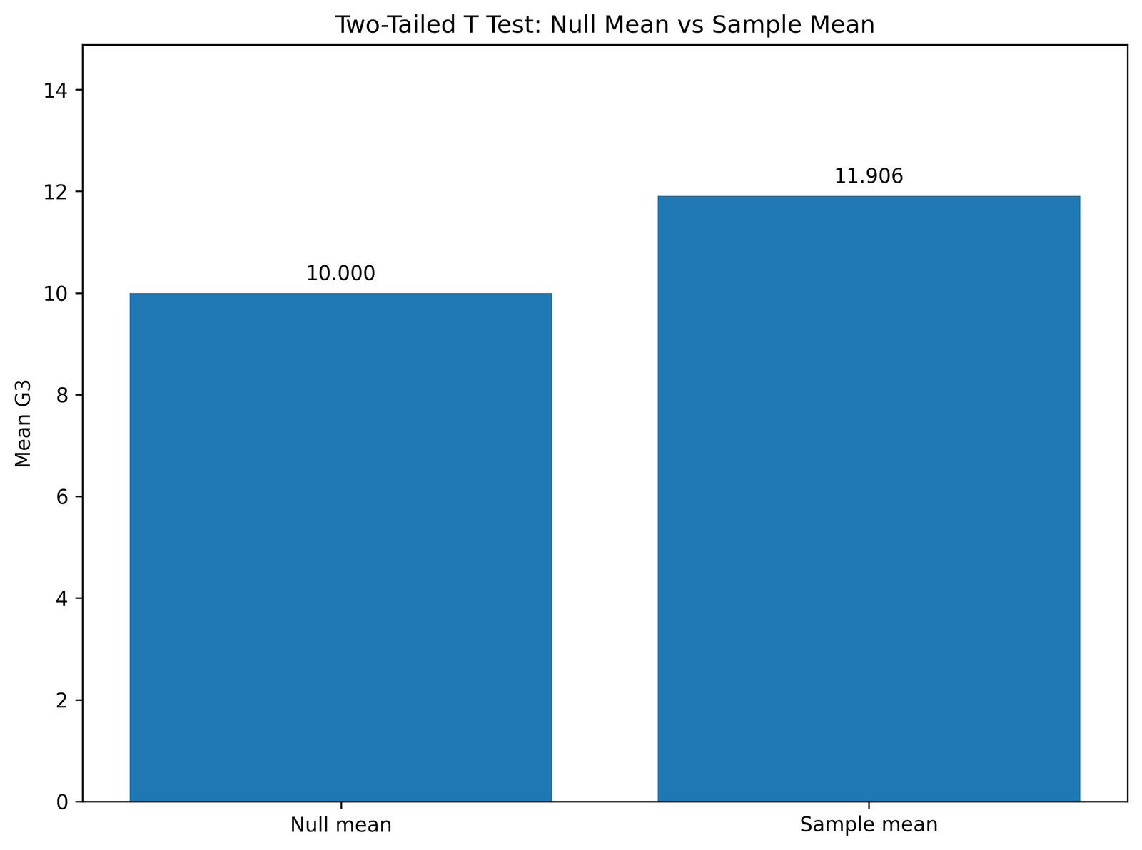
This chart isolates the main comparison. The null mean is 10, while the sample mean is approximately 11.906.
The observed direction is upward. However, the test remains two tailed because the alternative hypothesis is “different from 10,” not “greater than 10.”
Python Chart 3: Confidence Interval for Mean
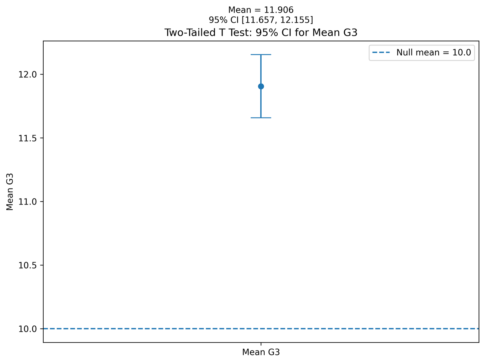
This chart shows the 95% confidence interval for the mean G3 score. Since the interval lies above 10, the null mean is not plausible at the 5% level.
The confidence interval reinforces the p-value decision and gives readers an interpretable range for the population mean.
Python Chart 4: Two Rejection Regions
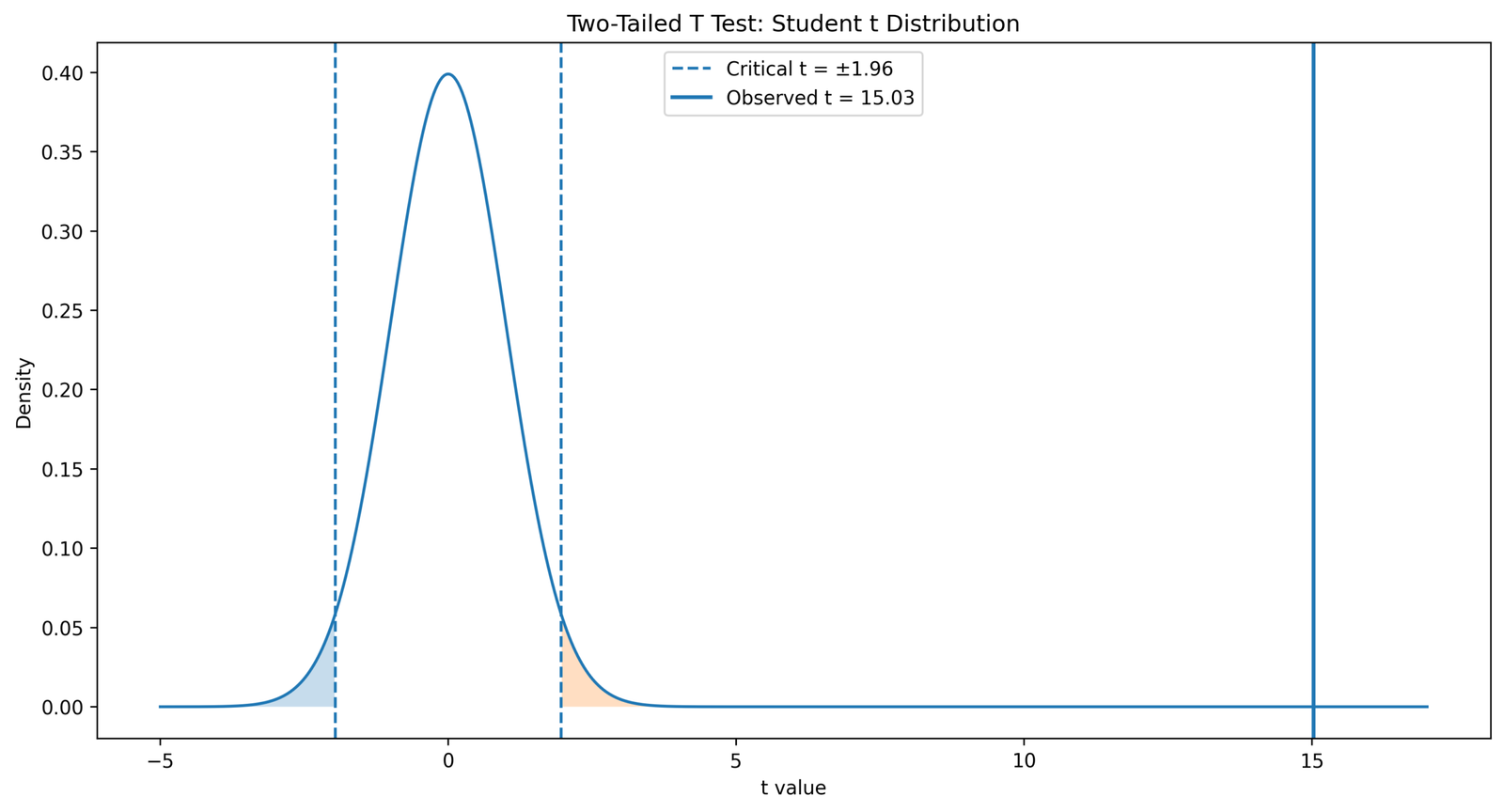
This is the most important visual for understanding a two tailed t test. The rejection region is split into the lower tail and upper tail.
The observed t statistic falls in the right rejection region. This means the sample mean is significantly higher than the null mean, even though the test allowed both directions.
Python Chart 5: Mean Difference
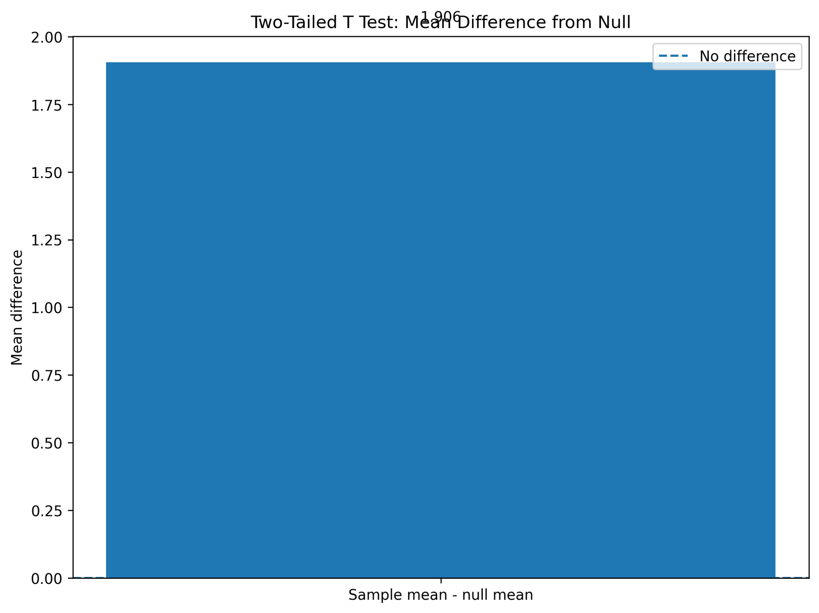
This chart explains the practical size of the result. The mean difference is about 1.906 grade points.
The result is statistically significant, but this chart helps readers see the size and direction of the difference in original grade units.
Python Chart 6: School Context Means
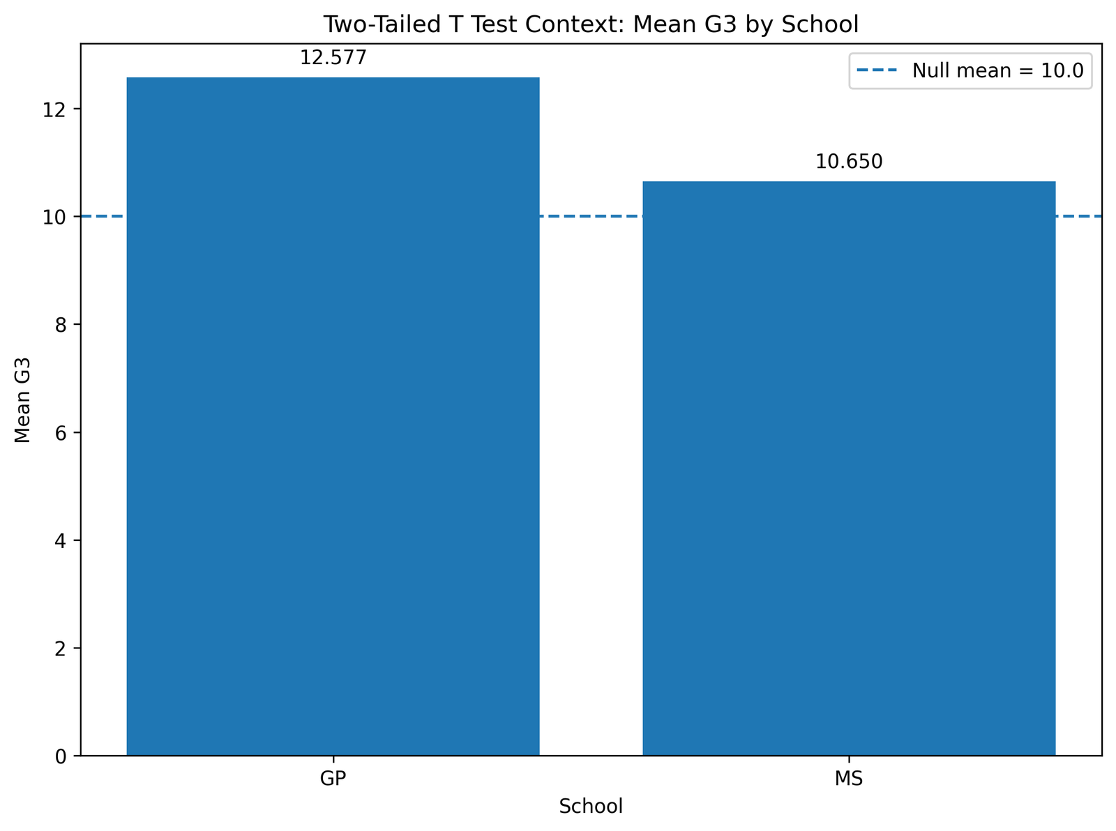
This chart shows how G3 differs descriptively by school. It helps readers understand where the outcome variable varies in the dataset.
The school comparison is contextual. The formal hypothesis test compares the overall G3 mean against 10.
Python Chart 7: Studytime Context Means
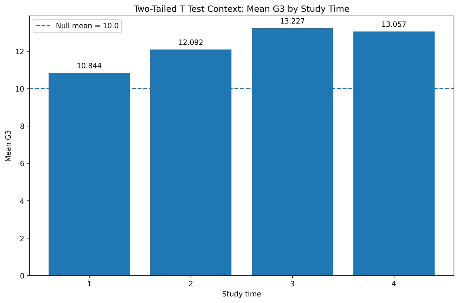
This chart shows G3 mean patterns across studytime categories. It supports descriptive interpretation of the outcome variable.
The chart should not be interpreted as the main t test. It is included to help explain the dataset around the tested variable.
Python Chart 8: Descriptives Table
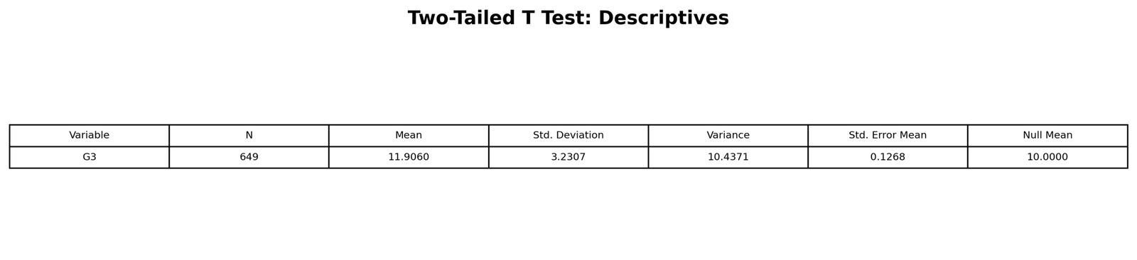
This table provides the descriptive statistics needed before interpreting the t test. It shows the sample size, mean, standard deviation and standard error.
The standard error is important because the t statistic divides the mean difference by the standard error.
Python Chart 9: Results Table
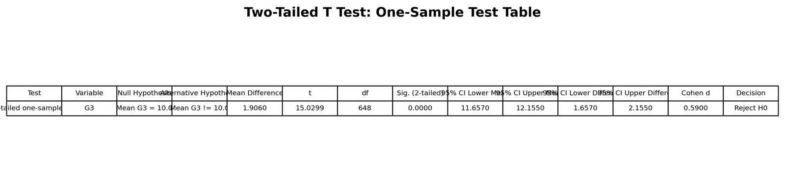
This is the main Python result table. It reports the statistic, degrees of freedom, p value, confidence interval and decision.
The p value is below .001, so the two tailed test rejects the null hypothesis.
Python Chart 10: Tail Decision Table
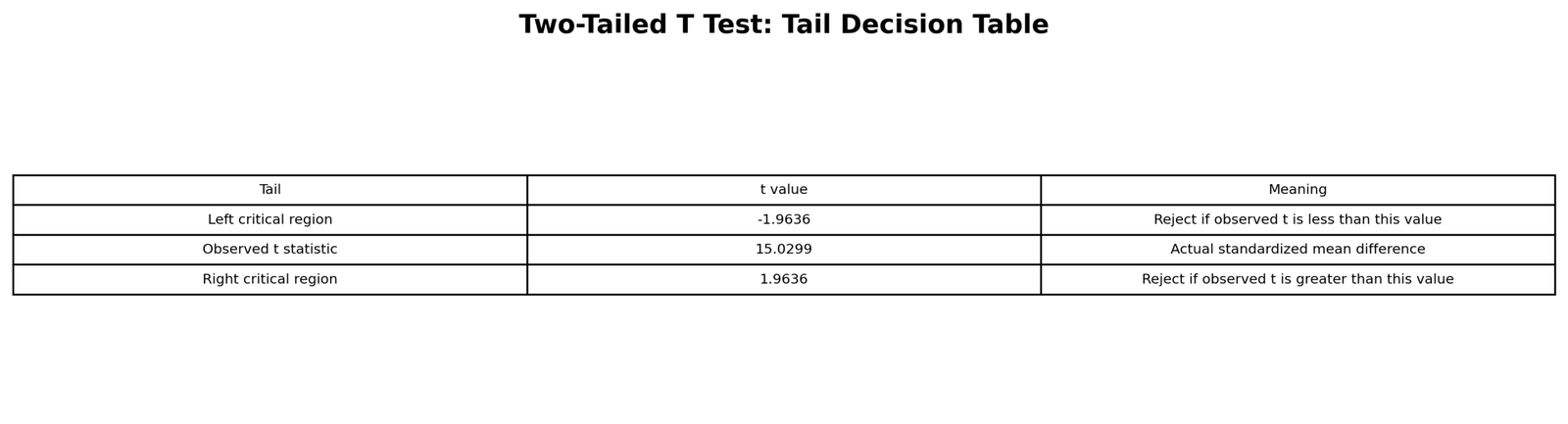
This decision table summarizes how the p value and tail structure lead to the final decision.
It shows that the test is significant because the observed t statistic is in the rejection region and the p value is below the alpha level.
R Chart-by-Chart Validation
The R charts validate the same two tailed t-test conclusion using an independent workflow. The same pattern appears: the sample mean is above the null mean, the confidence interval is above 10, the mean-difference interval is above zero, and the p value is statistically significant.
R Chart 1: G3 Distribution with Null and Sample Mean
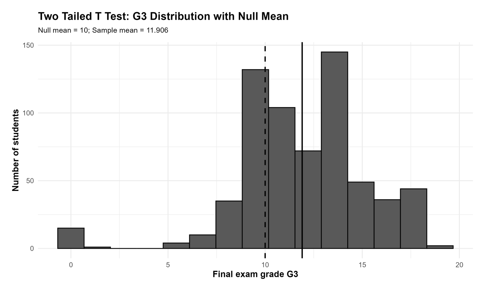
This R chart validates the Python and SPSS distribution pattern. The sample mean is above the null mean of 10.
The chart supports the conclusion that the t statistic is positive and large.
R Chart 2: Null Mean vs Sample Mean
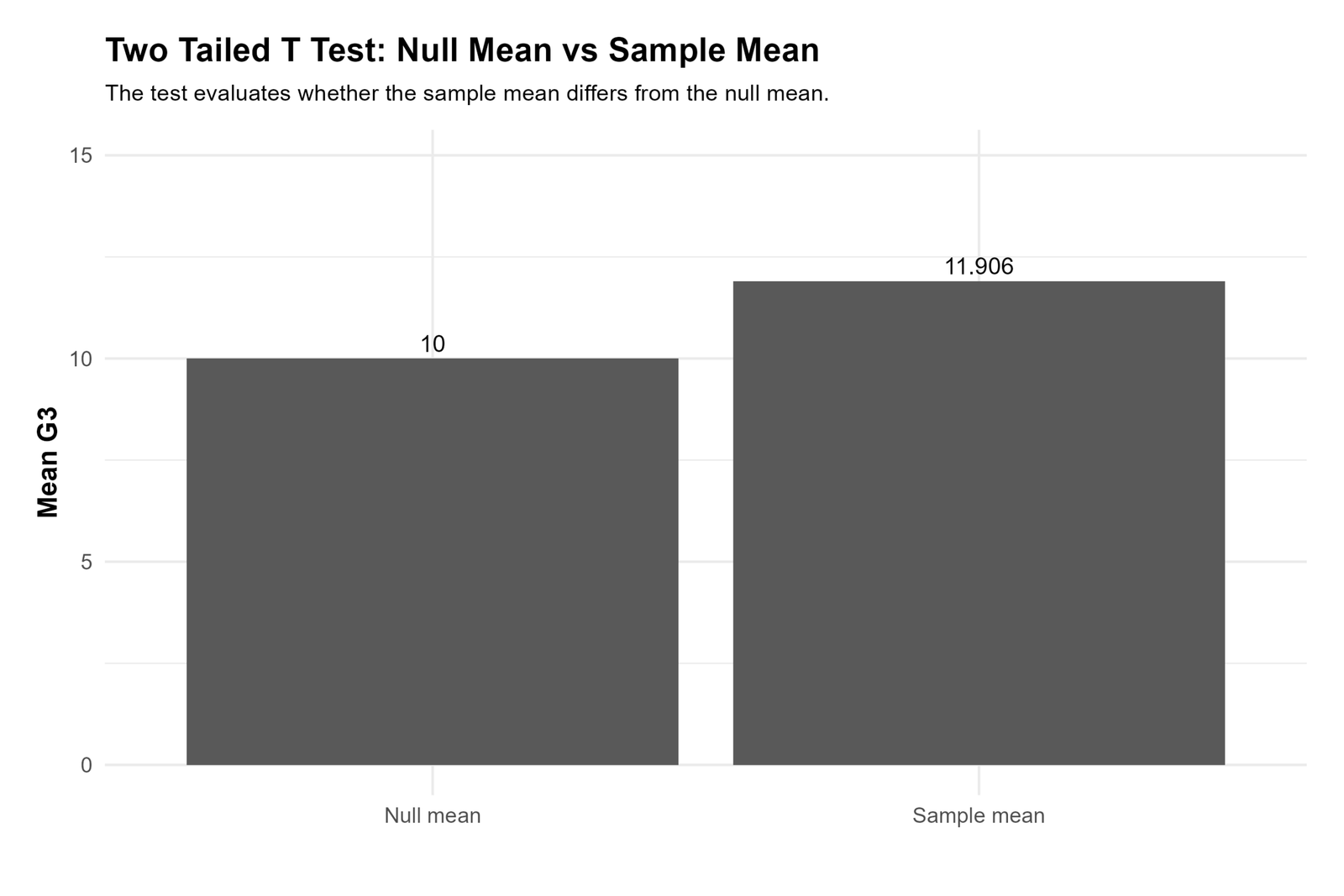
This chart confirms that the sample mean is higher than the null mean. The difference is about 1.906 points.
This visual explains the practical direction of the significant result.
R Chart 3: Mean Confidence Interval
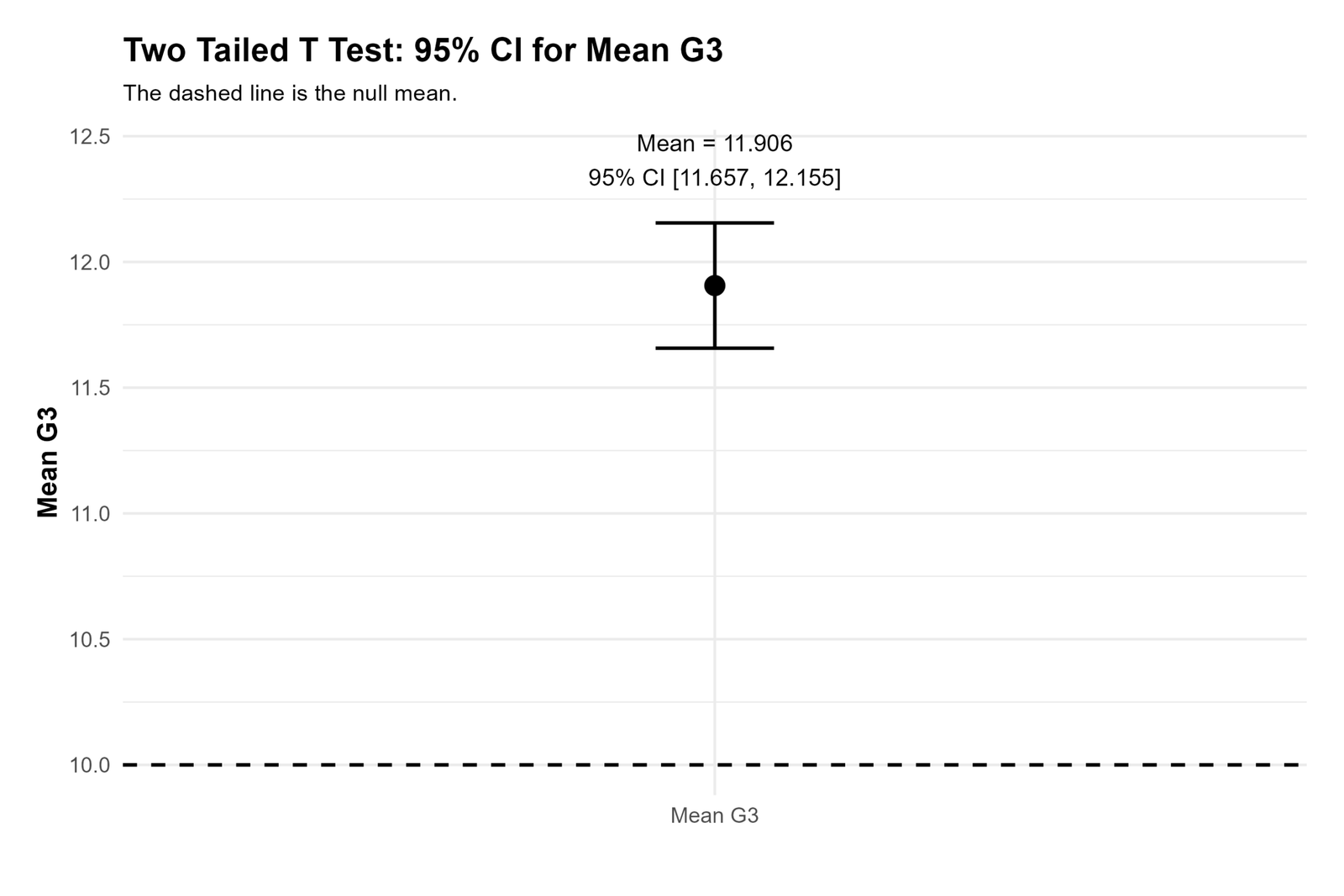
This chart shows the confidence interval for the G3 mean. Since the interval does not include 10, the two-tailed test rejects the null hypothesis.
The confidence interval validates the p-value result and gives a readable estimate of the mean range.
R Chart 4: T Statistic T Distribution Curve
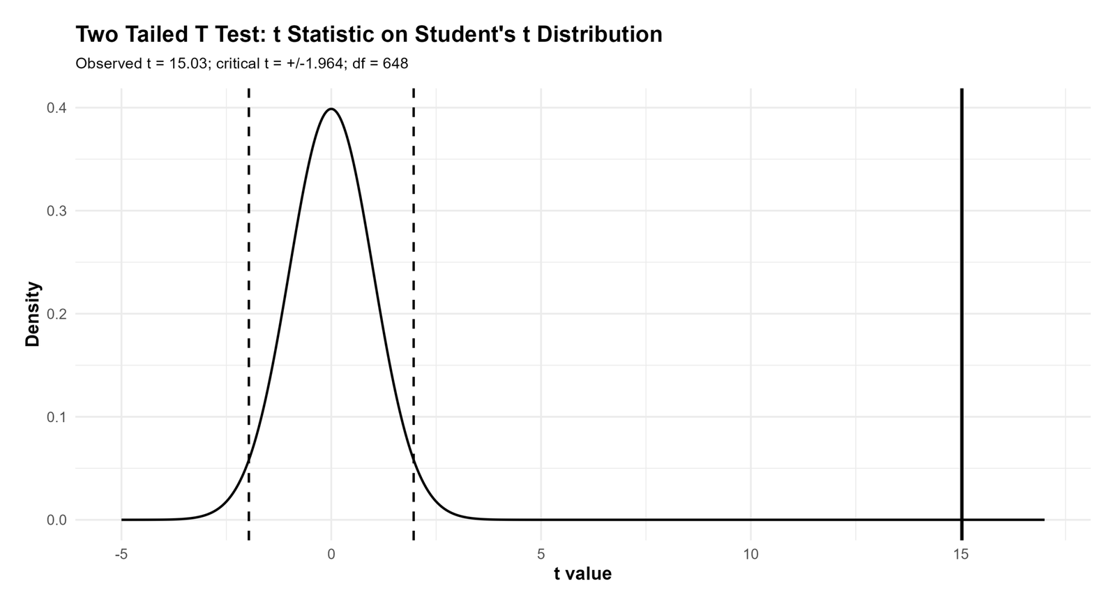
This R curve shows how the observed t statistic is judged against the t distribution. The value is far from zero and falls in the right rejection region.
The chart reinforces the idea that two tailed tests evaluate both tails even when the observed statistic is positive.
R Chart 5: Mean Difference Confidence Interval
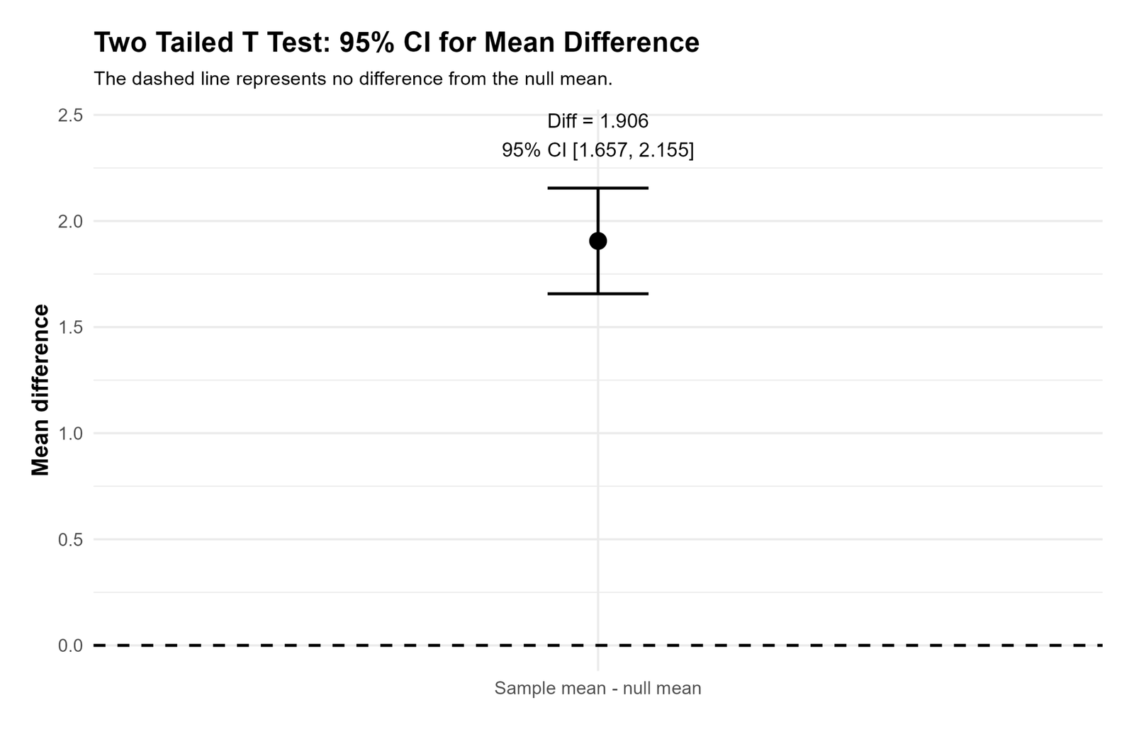
This chart validates that the mean difference is positive and statistically significant. The interval is above zero.
The chart is especially useful for reporting because it shows the direction and uncertainty of the difference.
R Chart 6: Mean G3 by School Context
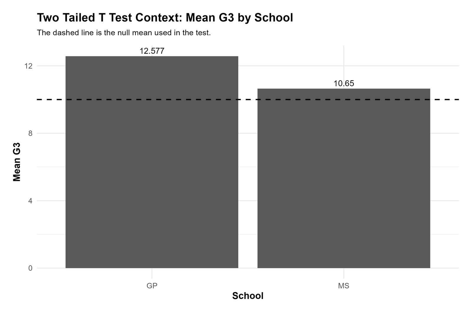
This chart shows descriptive differences in G3 by school. It helps explain the dataset but does not replace the one-sample t-test result.
The chart is included as a context visual for the tested outcome.
R Chart 7: Mean G3 by Studytime Context
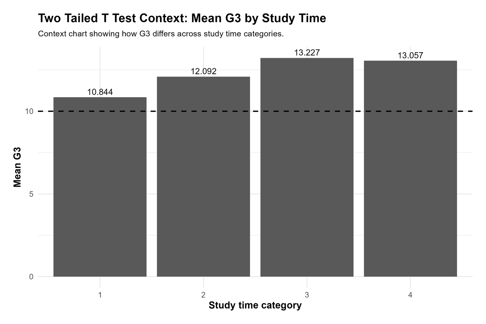
This chart validates the studytime context pattern. It gives additional interpretation for the G3 variable.
The formal two tailed decision remains based on the overall G3 mean compared with 10.
R Chart 8: Two Tailed T Test Main Result Table
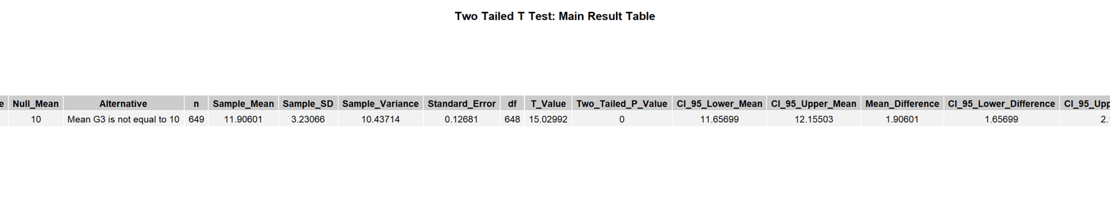
This table gives the R result summary: t statistic, degrees of freedom, p value, confidence interval and decision.
The R result confirms the same conclusion as SPSS and Python: reject the null hypothesis.
R Chart 9: Tail Decision Table
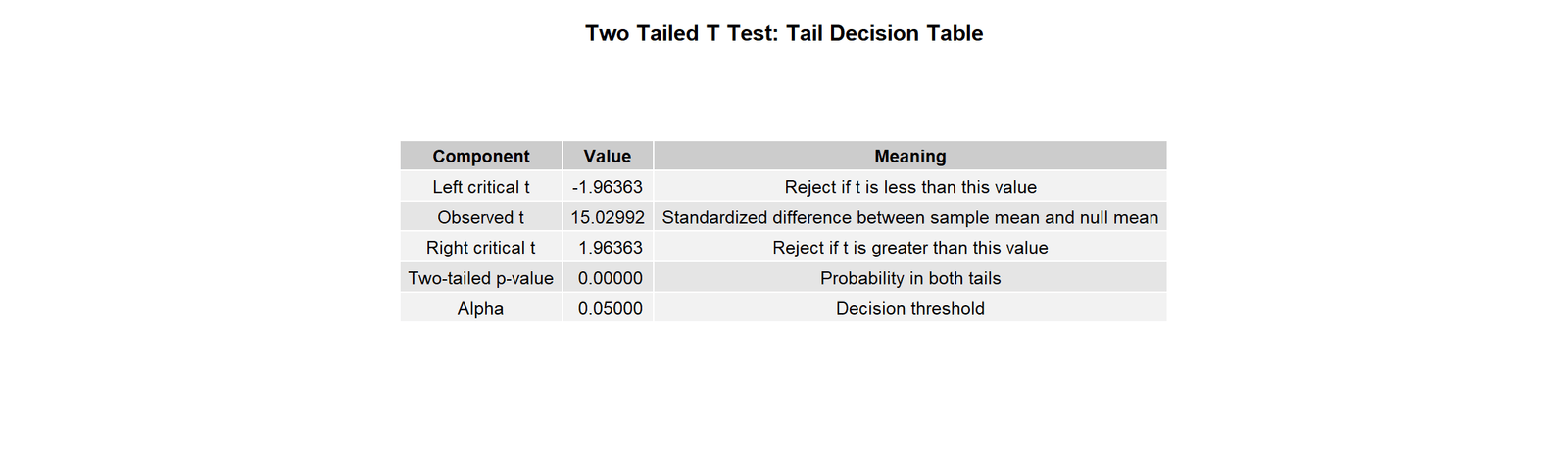
This table validates the decision logic. If p is below .05, reject the null hypothesis. If the confidence interval excludes the null value, the same decision is supported.
Both rules support rejection in this example.
R Chart 10: School Context Table

This table gives school-level descriptive summaries for G3. It helps readers understand the data context.
The formal hypothesis decision remains the one-sample two tailed t test comparing G3 with 10.
SPSS, R, Python and Excel Workflows for Two Tailed T Test
The same Two Tailed T Test can be reproduced in SPSS, R, Python and Excel. The software interface changes, but the statistical decision remains the same when the same variable, null mean, alpha level and two-tailed alternative are used.
SPSS Workflow
| Step | SPSS Action | Purpose |
|---|---|---|
| Open data | File > Open > Data | Load the dataset containing G3. |
| Choose test | Analyze > Compare Means > One-Sample T Test | Open the correct t-test dialog. |
| Select variable | Move G3 into Test Variable(s) | Set the numeric variable being tested. |
| Set test value | Enter 10 as Test Value | Define the null mean. |
| Read result | Sig. (2-tailed), t, df and CI | Make the final decision. |
| Export output | OUTPUT EXPORT | Save a PDF for reporting. |
R Workflow
| Step | R Action | Purpose |
|---|---|---|
| Read data | read.csv("dataset.csv") | Load the dataset. |
| Clean variable | g3 <- na.omit(df$G3) | Remove missing values. |
| Run test | t.test(g3, mu = 10, alternative = "two.sided") | Run the two tailed t test. |
| Read p value | result$p.value | Determine significance. |
| Read CI | result$conf.int | Interpret the plausible mean range. |
Python Workflow
| Step | Python Action | Purpose |
|---|---|---|
| Read data | pandas.read_csv() | Load the dataset into a DataFrame. |
| Clean variable | dropna() | Keep valid G3 cases. |
| Run test | stats.ttest_1samp(g3, popmean=10) | Calculate t statistic and two-sided p value. |
| Calculate CI | stats.t.ppf() | Build 95% confidence interval. |
| Plot decision | matplotlib | Show two rejection regions and mean comparison. |
Excel Workflow
| Excel Task | Formula or Tool | Purpose |
|---|---|---|
| Count sample size | =COUNT(range) | Get n. |
| Calculate mean | =AVERAGE(range) | Get sample mean. |
| Calculate standard deviation | =STDEV.S(range) | Get sample standard deviation. |
| Calculate standard error | =STDEV.S(range)/SQRT(COUNT(range)) | Get standard error. |
| Calculate t statistic | =(AVERAGE(range)-10)/SE | Calculate t. |
| Calculate two-tailed p value | =T.DIST.2T(ABS(t),df) | Make the p-value decision. |
Code Blocks for Two Tailed T Test
SPSS Syntax for Two Tailed T Test
* Two tailed one-sample t test in SPSS.
* Test variable: G3.
* Null mean: 10.

TITLE "Two Tailed T Test for G3 Against Null Mean 10".

T-TEST
  /TESTVAL=10
  /VARIABLES=G3
  /MISSING=ANALYSIS
  /CRITERIA=CI(.95).

EXAMINE VARIABLES=G3
  /PLOT BOXPLOT HISTOGRAM NPPLOT
  /STATISTICS DESCRIPTIVES
  /CINTERVAL 95
  /MISSING LISTWISE
  /NOTOTAL.

MEANS TABLES=G3 BY school
  /CELLS MEAN COUNT STDDEV SEMEAN.

MEANS TABLES=G3 BY studytime
  /CELLS MEAN COUNT STDDEV SEMEAN.

OUTPUT EXPORT
  /CONTENTS EXPORT=VISIBLE
  /PDF DOCUMENTFILE="Two-Tailed-T-Test-SPSS-Output.pdf".
Python Code for Two Tailed T Test
import pandas as pd
import numpy as np
from scipy import stats

df = pd.read_csv("dataset.csv")

df["G3"] = pd.to_numeric(df["G3"], errors="coerce")
g3 = df["G3"].dropna()

mu0 = 10
alpha = 0.05

result = stats.ttest_1samp(g3, popmean=mu0)

n = len(g3)
mean_g3 = g3.mean()
sd_g3 = g3.std(ddof=1)
se_g3 = sd_g3 / np.sqrt(n)
dfree = n - 1

t_crit = stats.t.ppf(1 - alpha / 2, dfree)
ci_low = mean_g3 - t_crit * se_g3
ci_high = mean_g3 + t_crit * se_g3
mean_diff = mean_g3 - mu0

decision = "Reject H0" if result.pvalue < alpha else "Fail to reject H0"

print("Two Tailed T Test")
print("n:", n)
print("sample mean:", mean_g3)
print("null mean:", mu0)
print("mean difference:", mean_diff)
print("t statistic:", result.statistic)
print("df:", dfree)
print("two-tailed p value:", result.pvalue)
print("95% CI:", ci_low, ci_high)
print("decision:", decision)
R Code for Two Tailed T Test
# Two tailed one-sample t test in R

df <- read.csv("dataset.csv")

df$G3 <- as.numeric(df$G3)
g3 <- na.omit(df$G3)

result <- t.test(
  g3,
  mu = 10,
  alternative = "two.sided",
  conf.level = 0.95
)

print(result)

# Extract values
result$statistic
result$parameter
result$p.value
result$conf.int
result$estimate

# Descriptive values
n <- length(g3)
mean_g3 <- mean(g3)
sd_g3 <- sd(g3)
se_g3 <- sd_g3 / sqrt(n)
mean_diff <- mean_g3 - 10

data.frame(
  n = n,
  mean = mean_g3,
  sd = sd_g3,
  se = se_g3,
  mean_difference = mean_diff,
  t = as.numeric(result$statistic),
  df = as.numeric(result$parameter),
  p_value = result$p.value,
  ci_low = result$conf.int[1],
  ci_high = result$conf.int[2]
)
Excel Formulas for Two Tailed T Test
Sample size:
=COUNT(sample_range)

Sample mean:
=AVERAGE(sample_range)

Sample standard deviation:
=STDEV.S(sample_range)

Standard error:
=STDEV.S(sample_range)/SQRT(COUNT(sample_range))

Mean difference:
=AVERAGE(sample_range)-10

t statistic:
=(AVERAGE(sample_range)-10)/(STDEV.S(sample_range)/SQRT(COUNT(sample_range)))

Degrees of freedom:
=COUNT(sample_range)-1

Two-tailed critical value:
=T.INV.2T(0.05,df_cell)

Two-tailed p value:
=T.DIST.2T(ABS(t_cell),df_cell)

Decision:
=IF(p_value_cell<0.05,"Reject H0","Fail to reject H0")
APA Reporting Wording
When reporting a Two Tailed T Test, include the test type, sample size or degrees of freedom, sample mean, null mean, t statistic, p value, confidence interval and final interpretation. The wording should make clear that the alternative hypothesis was non-directional.
APA-style report: A two-tailed one-sample t test was conducted to determine whether the mean G3 final grade differed from 10. The sample mean was significantly higher than the null value, M = 11.91, t(648) = 15.03, p < .001, 95% CI [11.66, 12.16]. Therefore, the null hypothesis was rejected.
Short reporting version: The two tailed t test showed that mean G3 was significantly different from 10, t(648) = 15.03, p < .001. The observed mean was higher than the null mean.
Common Mistakes
| Mistake | Why It Is Wrong | Correct Practice |
|---|---|---|
| Changing from two tailed to one tailed after seeing the result | This inflates the chance of a false positive. | Choose the tail direction before analysis. |
| Forgetting to double the one-tail probability | A two-tailed p value includes both tails. | Use p = 2 × P(T ≥ |t|). |
| Using the wrong critical value | Two-tailed tests split alpha across two tails. | Use tα/2,df or Excel T.INV.2T. |
| Reporting only p value | The p value does not show the estimated mean range. | Report mean, t, df, p value and confidence interval. |
| Calling the result “greater than” without explaining the hypothesis | The two-tailed hypothesis is non-directional. | Say the mean was significantly different, then describe the observed direction. |
| Ignoring assumptions | T tests assume numeric outcome, independent observations and approximate normality of the sampling distribution. | Check descriptive statistics, plots and sample size before reporting. |
When to Use Two Tailed T Test
Use a Two Tailed T Test when the research question is about whether a mean is different from a value, and a difference in either direction would matter.
| Research Question | Correct Tail | Example Hypothesis |
|---|---|---|
| Is the mean different from 10? | Two tailed | H1: μ ≠ 10 |
| Is the mean greater than 10? | Right tailed | H1: μ > 10 |
| Is the mean less than 10? | Left tailed | H1: μ < 10 |
| Would both lower and higher values matter? | Two tailed | Use two rejection regions. |
Best practice: Use a two tailed t test unless there is a strong theoretical, practical or preregistered reason to use a one tailed test.
Downloads and Resources
Use these resources to reproduce the Two Tailed T Test workflow. Replace the placeholder links with final hosted file URLs after uploading the dataset, scripts, syntax files, workbook and output PDFs to WordPress Media Library.
Download Dataset
Practice dataset with G3 final grade and context variables.
Download SPSS Syntax and Output PDF
SPSS one-sample two tailed t test syntax with PDF export.
Download Python Script
Python code for two tailed t test, p value, confidence interval and charts.
Download R Script and Excel Workbook
R validation code and Excel formulas for two-tailed p value and critical value.
FAQs About Two Tailed T Test
What is a two tailed t test?
A two tailed t test checks whether a sample mean is significantly different from a null mean in either direction, lower or higher.
When should I use a two tailed t test?
Use a two tailed t test when the alternative hypothesis is non-directional, such as μ ≠ μ0, and a difference in either direction would be meaningful.
What is the two tailed t test formula?
The one-sample formula is t = (sample mean - null mean) / (sample standard deviation / square root of n).
How do I calculate p value for two tailed t test?
Calculate the t statistic, take its absolute value, find the upper-tail probability, and multiply by 2. In software, use the two-sided or two-tailed option.
What is the difference between one tailed and two tailed t test?
A one tailed t test checks only one direction. A two tailed t test checks both directions and splits the alpha level across both tails.
What is the rejection region for a two tailed t test?
The rejection region is split between the left tail and right tail of the t distribution. For alpha = .05, each tail contains .025.
How do I report a two tailed t test?
Report the sample mean, null value, t statistic, degrees of freedom, two-tailed p value, confidence interval and conclusion.
What does Sig. (2-tailed) mean in SPSS?
Sig. (2-tailed) is the two-tailed p value. If it is below .05, the test result is statistically significant at the 5% level.

