Repeated-Measures ANOVA Assumption Test
Mauchly’s Test of Sphericity is used in repeated-measures ANOVA to check whether the sphericity assumption is reasonable before interpreting the ordinary within-subjects F-test. This complete guide explains the Mauchly test formula, null hypothesis, interpretation, SPSS output, R workflow, Python validation, Excel checking method, charts and APA-style reporting using the student-por.csv dataset with repeated grade measurements G1, G2 and G3.
Google AdSense top placement reserved here
Quick Answer: Mauchly’s Test of Sphericity Result
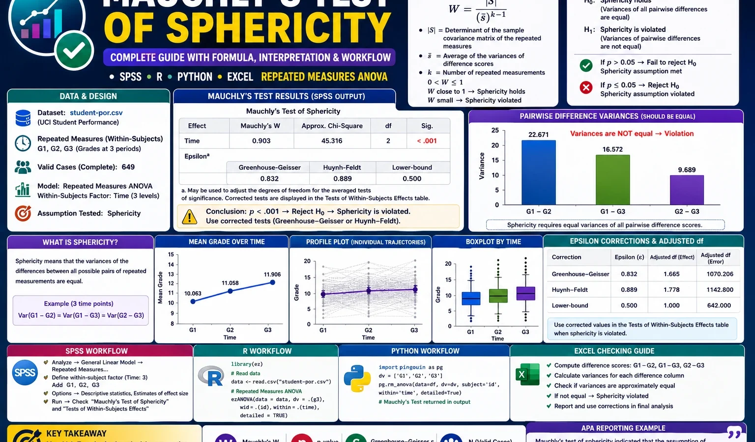
The Mauchly’s Test of Sphericity result for the repeated grade measurements G1, G2 and G3 was significant. The test produced Mauchly’s W = .827, χ²(2) = 122.814 and p < .001. Therefore, the assumption of sphericity was violated. Because of this violation, the repeated-measures ANOVA should be interpreted with a corrected row such as Greenhouse-Geisser or Huynh-Feldt, instead of relying only on the sphericity-assumed row.
Final report sentence: Mauchly’s Test indicated that the assumption of sphericity was violated, W = .827, χ²(2) = 122.814, p < .001. Therefore, a corrected repeated-measures ANOVA row was used. The Huynh-Feldt corrected result remained significant, F(1.709, 1107.581) = 36.287, p < .001, partial η² = .053, showing that mean grades changed significantly across G1, G2 and G3.
Important SPSS note: SPSS displays very small p-values as .000. In a thesis, assignment, research article or APA-style report, do not write p = .000. Write p < .001.
What Is Mauchly’s Test of Sphericity?
Mauchly’s Test of Sphericity is an assumption test used mainly with repeated-measures ANOVA. Repeated-measures ANOVA is used when the same subjects are measured more than two times, or when the same person contributes scores under three or more related conditions. In this worked example, each student has three related grade measurements: G1, G2 and G3.
The sphericity assumption concerns the pattern of variances among the pairwise difference scores. In simple words, repeated-measures ANOVA expects the differences between repeated measurements to have similar variances. For three grade measurements, the relevant differences are G2 − G1, G3 − G2 and G3 − G1. If these difference-score variances are too unequal, the standard repeated-measures ANOVA degrees of freedom can become too optimistic. That can make a test appear more precise than it really is.
Mauchly’s Test checks this assumption statistically. If Mauchly’s Test is not significant, the sphericity assumption is usually treated as acceptable. If Mauchly’s Test is significant, sphericity is considered violated and a correction should be used. Common corrections include the Greenhouse-Geisser Correction, the Huynh-Feldt Correction and the lower-bound correction.
Plain-language meaning: Mauchly’s Test of Sphericity asks whether the repeated-measures ANOVA can safely use the ordinary sphericity-assumed degrees of freedom. In this example, the answer is no, because p < .001. The analysis should therefore report a corrected row.
When Should You Use Mauchly’s Test of Sphericity?
Use Mauchly’s Test of Sphericity when the design has a within-subject factor with at least three levels. It is not needed for a simple paired-samples t-test because with only two repeated measurements, the sphericity assumption is automatically satisfied. It is most relevant in education, psychology, medical trials, training evaluation, longitudinal measurement and experimental designs where the same people are measured repeatedly.
| Research situation | Use Mauchly’s Test? | Reason |
|---|---|---|
| Three exam scores from the same students | Yes | There are three related measurements, so repeated-measures ANOVA needs a sphericity check. |
| Pre-test, post-test and follow-up score | Yes | The same subjects are measured at three time points. |
| Four repeated treatment conditions | Yes | There are more than two within-subject levels. |
| Only two paired measurements | No | Sphericity is automatically met with two repeated levels. |
| Independent groups ANOVA | No | Use variance-related tests such as Brown-Forsythe Test, Levene’s test or related independent-group assumption checks. |
Mauchly’s Test of Sphericity Formula and Logic
The full mathematical calculation of Mauchly’s Test of Sphericity is based on the covariance matrix of the orthonormalized transformed repeated measures. In applied data analysis, most students and researchers do not calculate Mauchly’s W by hand. SPSS, R and Python calculate it from the repeated-measures covariance structure.
The practical idea can be understood through the pairwise difference scores. If the variances of the pairwise differences are similar, sphericity is more plausible. If those variances are quite different, sphericity becomes doubtful. In this dataset, the difference variances were not equal:
| Difference score | Mean difference | Standard deviation | Variance | Interpretation |
|---|---|---|---|---|
| G2 − G1 | .1710 | 1.47929 | 2.188 | Small average increase from first to second grade measurement. |
| G3 − G2 | .3359 | 1.27824 | 1.634 | Average increase from second grade measurement to final grade. |
| G3 − G1 | .5069 | 1.82076 | 3.315 | Largest total average increase from first grade measurement to final grade. |
The difference variance for G3 − G1 is much larger than the variance for G3 − G2. This unequal pattern explains why Mauchly’s Test became significant in the SPSS, R and Python workflows.
Null Hypothesis and Alternative Hypothesis
| Hypothesis | Meaning | Decision in this example |
|---|---|---|
| H0 | The sphericity assumption is satisfied. The covariance pattern is suitable for the ordinary repeated-measures ANOVA row. | Rejected because p < .001. |
| H1 | The sphericity assumption is violated. A correction should be used for the repeated-measures ANOVA. | Supported by the significant Mauchly’s Test result. |
Google AdSense middle placement reserved here
Dataset and Repeated-Measures Model Used
This tutorial uses the student-por.csv student performance dataset. The repeated measures are G1, G2 and G3. These are grade measurements recorded for the same students, so the design is a within-subject repeated-measures design.
| Item | Value used | Explanation |
|---|---|---|
| Dataset | student-por.csv | Student performance dataset used for R, Python and SPSS verification. |
| Sample size | 649 | All 649 students had valid G1, G2 and G3 values. |
| Repeated measures | G1, G2, G3 | Three grade measurements from the same students. |
| Within-subject factor | GradeTime | Repeated factor with three levels. |
| Assumption test | Mauchly’s Test of Sphericity | Tests whether the sphericity assumption is satisfied. |
| Main repeated-measures test | Repeated-measures ANOVA | Tests whether mean grade changes across G1, G2 and G3. |
External dataset source: UCI Machine Learning Repository: Student Performance dataset.
Verified Results in SPSS, R and Python
The analysis was reproduced in SPSS, R and Python. The three workflows confirmed the same conclusion: Mauchly’s Test of Sphericity is significant, meaning the sphericity assumption is violated for the repeated grade measurements.
Descriptive Statistics for G1, G2 and G3
| Repeated measure | N | Minimum | Maximum | Mean | Standard deviation | Short interpretation |
|---|---|---|---|---|---|---|
| G1 | 649 | 0 | 19 | 11.40 | 2.745 | First grade measurement; lowest mean among the three repeated scores. |
| G2 | 649 | 0 | 19 | 11.57 | 2.914 | Second grade measurement; slightly higher than G1. |
| G3 | 649 | 0 | 19 | 11.91 | 3.231 | Final grade measurement; highest mean and largest spread. |
Mauchly’s Test of Sphericity Table
| Statistic | Verified value | Interpretation |
|---|---|---|
| Mauchly’s W | .827 | The covariance pattern is not perfectly spherical. |
| Approx. Chi-square | 122.814 | Large chi-square statistic for the sphericity test. |
| df | 2 | Degrees of freedom for the Mauchly test with three repeated measures. |
| Sig. | .000 | Report as p < .001; sphericity is violated. |
Epsilon Correction Values
| Correction | Epsilon value | Meaning |
|---|---|---|
| Greenhouse-Geisser | .853 | A conservative correction used after sphericity violation. |
| Huynh-Feldt | .855 | A slightly less conservative correction; very close to Greenhouse-Geisser in this example. |
| Lower-bound | .500 | The strictest correction for three repeated measurements. |
Tests of Within-Subjects Effects
| Correction row | Effect df | Error df | F | p-value | Partial η² | Decision |
|---|---|---|---|---|---|---|
| Sphericity assumed | 2.000 | 1296.000 | 36.287 | < .001 | .053 | Significant, but not preferred because Mauchly’s Test is significant. |
| Greenhouse-Geisser | 1.705 | 1104.961 | 36.287 | < .001 | .053 | Significant corrected result. |
| Huynh-Feldt | 1.709 | 1107.581 | 36.287 | < .001 | .053 | Significant corrected result; used in the main reporting sentence here. |
| Lower-bound | 1.000 | 648.000 | 36.287 | < .001 | .053 | Still significant even with the strictest correction. |
Main interpretation: The repeated grade means changed significantly across G1, G2 and G3. However, because Mauchly’s Test of Sphericity was significant, the corrected repeated-measures ANOVA row should be used. The conclusion remains statistically significant under Greenhouse-Geisser, Huynh-Feldt and lower-bound corrections.
R Charts for Mauchly’s Test of Sphericity
The R workflow produced eight charts that explain the repeated-measures pattern, the sphericity issue and the correction values. These charts are useful for teaching because Mauchly’s Test is easier to understand when the repeated grade pattern and pairwise difference variances are visible.
1. Mean Grade Profile Across G1, G2 and G3

The mean profile shows a steady increase from G1 = 11.40 to G2 = 11.57 and then to G3 = 11.91. This upward trend explains why the repeated-measures ANOVA found a significant within-subject effect. Mauchly’s Test does not test whether the means are different; it checks whether the repeated-measures covariance structure is suitable for the ordinary ANOVA row.
2. Grade Distribution Boxplot

The boxplot shows that the final grade measurement has a slightly higher center and a wider spread. The lower outliers around zero are visible, especially in G3. These distributional features are not the same as sphericity, but they help explain why the repeated grade measurements are not perfectly uniform across time.
3. Pairwise Difference Variances for Sphericity Check

This is the most important explanatory chart for Mauchly’s Test of Sphericity. The variance for G3 − G1 is 3.315, while the variance for G3 − G2 is only 1.634. This unequal pattern supports the significant Mauchly result and explains why a corrected ANOVA row is needed.
4. Mauchly’s Test Summary

The summary chart highlights the main result: W = .827, χ² = 122.814 and p < .001. Since the p-value is below .05, the null hypothesis of sphericity is rejected.
5. Sphericity Correction Epsilon Values

The epsilon chart shows that Greenhouse-Geisser = .853 and Huynh-Feldt = .855. These values are very close, so both corrected rows lead to the same practical conclusion. The lower-bound correction is .500, which is the most conservative option for three repeated measures.
6. Sample Student Grade Trajectories

The trajectory chart shows that not every student follows the same pattern. Some students improve, some remain stable and some decline. The bold average line still rises across G1, G2 and G3. This is why the repeated-measures effect is significant even though individual trajectories vary.
7. Histograms of G1, G2 and G3

The histograms show that the three grade measurements have broadly similar score ranges but not identical distribution shapes. G3 has more spread and visible low-end values. The histograms help readers understand the raw score pattern before interpreting the Mauchly and ANOVA tables.
8. Pairwise Difference Score Distributions

The difference-score histograms provide a direct visual explanation of sphericity. Mauchly’s Test is related to how these difference scores vary. Since the difference distributions do not have equal variance, the test detects a sphericity violation.
Python Validation Charts for Mauchly’s Test of Sphericity
The Python workflow independently reproduced the Mauchly result, epsilon values, corrected degrees of freedom and repeated-measures ANOVA effect. This validation is useful because it shows that the result does not depend on only one software package.
1. Python Mean Grade Profile

The Python mean profile confirms the same increasing pattern found in R and SPSS. The final grade mean is highest, and the error bars show uncertainty around each mean estimate.
2. Python Grade Distribution Boxplot

The Python boxplot confirms that G3 has a higher center and wider spread than the earlier grade measurements. This supports the descriptive interpretation of the repeated-measures model.
3. Python Pairwise Difference Variances

The Python variance chart matches the R chart: 2.188, 3.315 and 1.634. This repeated confirmation is important because the pairwise difference variance pattern is the most intuitive way to understand the sphericity violation.
4. Python Mauchly Test Summary

The Python result confirms the SPSS and R conclusion: the sphericity assumption is violated. Since p < .001, corrected repeated-measures ANOVA degrees of freedom are required.
5. Python Epsilon Values

The Python epsilon chart confirms the same correction values: Greenhouse-Geisser = .853, Huynh-Feldt = .855 and Lower-bound = .500.
6. Python Sample Student Trajectories

The trajectory chart shows strong individual variation. This is normal in educational data. Repeated-measures ANOVA tests the average pattern while accounting for the fact that the same students are measured repeatedly.
7. Python Histograms of G1, G2 and G3

The Python histograms confirm that the grade distributions are concentrated around the middle of the scale but include low outlying values. These charts are useful for describing the dataset before presenting the assumption test.
8. Python Pairwise Difference Score Histograms

The pairwise difference histograms show that the differences are centered near small positive values, but their spreads are not the same. This supports the significant Mauchly’s Test result.
9. Python Corrected Degrees of Freedom Comparison

This chart explains what the correction actually does. The F statistic remains the same, but the degrees of freedom are reduced. The Huynh-Feldt effect df becomes 1.709 and the error df becomes 1107.581.
10. Python Repeated-Measures ANOVA Effect Summary

The Python ANOVA summary confirms F = 36.287. Since the corrected p-value remains below .001, the repeated grade effect is statistically significant even after the sphericity correction.
How to Run Mauchly’s Test of Sphericity in SPSS, R, Python and Excel
Mauchly’s Test of Sphericity in SPSS
SPSS reports Mauchly’s Test automatically when repeated-measures ANOVA is run through the General Linear Model repeated-measures procedure. The key output tables are Mauchly’s Test of Sphericity, Tests of Within-Subjects Effects and the epsilon correction values.
* Mauchly's Test of Sphericity in SPSS.

GET DATA
 /TYPE=TXT
 /FILE='D:\low kda score priority basis posts\first post\Mauchly Test of Sphericity\student-por.csv'
 /ENCODING='UTF8'
 /DELCASE=LINE
 /DELIMITERS=","
 /QUALIFIER='"'
 /ARRANGEMENT=DELIMITED
 /FIRSTCASE=2
 /VARIABLES=
 school A40
 sex A20
 age F8.0
 address A20
 famsize A20
 Pstatus A20
 Medu F8.0
 Fedu F8.0
 Mjob A40
 Fjob A40
 reason A40
 guardian A40
 traveltime F8.0
 studytime F8.0
 failures F8.0
 schoolsup A40
 famsup A40
 paid A40
 activities A40
 nursery A40
 higher A40
 internet A40
 romantic A40
 famrel F8.0
 freetime F8.0
 goout F8.0
 Dalc F8.0
 Walc F8.0
 health F8.0
 absences F8.0
 G1 F8.0
 G2 F8.0
 G3 F8.0.
CACHE.
EXECUTE.

GLM G1 G2 G3
 /WSFACTOR=GradeTime 3 Polynomial
 /MEASURE=Grade
 /METHOD=SSTYPE(3)
 /PRINT=DESCRIPTIVE ETASQ
 /CRITERIA=ALPHA(.05)
 /WSDESIGN=GradeTime.
Mauchly’s Test of Sphericity in R
In R, the workflow is to read the dataset, reshape the data from wide to long format and run a repeated-measures ANOVA function that reports Mauchly’s Test and sphericity corrections.
install.packages(c("tidyverse", "ez"))

library(tidyverse)
library(ez)

base_dir <- "D:/low kda score priority basis posts/first post/Mauchly Test of Sphericity"
student <- read.csv(file.path(base_dir, "student-por.csv"), sep = ",")

clean_data <- student %>%
  mutate(subject_id = row_number()) %>%
  filter(!is.na(G1), !is.na(G2), !is.na(G3))

long_data <- clean_data %>%
  select(subject_id, G1, G2, G3) %>%
  pivot_longer(cols = c(G1, G2, G3),
               names_to = "GradeTime",
               values_to = "Grade") %>%
  mutate(
    subject_id = factor(subject_id),
    GradeTime = factor(GradeTime, levels = c("G1", "G2", "G3"))
  )

mauchly_result <- ezANOVA(
  data = long_data,
  dv = Grade,
  wid = subject_id,
  within = GradeTime,
  detailed = TRUE,
  type = 3
)

print(mauchly_result)
Mauchly’s Test of Sphericity in Python
Python can reproduce the same logic by calculating the repeated-measures covariance structure and sphericity-related correction values. The validation workflow used NumPy, pandas, SciPy and Matplotlib to reproduce the Mauchly W value, chi-square approximation, epsilon values and charts.
import numpy as np
import pandas as pd
from scipy.stats import chi2

data = pd.read_csv(
    r"D:\low kda score priority basis posts\first post\Mauchly Test of Sphericity\student-por.csv"
)

X = data[["G1", "G2", "G3"]].dropna().to_numpy(dtype=float)
n, k = X.shape
p = k - 1

cov_matrix = np.cov(X, rowvar=False, ddof=1)

C = np.array([
    [1 / np.sqrt(2),  1 / np.sqrt(6)],
    [-1 / np.sqrt(2), 1 / np.sqrt(6)],
    [0,              -2 / np.sqrt(6)]
])

contrast_cov = C.T @ cov_matrix @ C

mauchly_w = np.linalg.det(contrast_cov) / ((np.trace(contrast_cov) / p) ** p)

correction_factor = 1 - ((2 * p**2 + p + 2) / (6 * p * (n - 1)))
chi_square_value = -((n - 1) * correction_factor * np.log(mauchly_w))
df = int((p * (p + 1) / 2) - 1)
p_value = chi2.sf(chi_square_value, df)

print(mauchly_w, chi_square_value, df, p_value)
Mauchly’s Test of Sphericity in Excel
Excel is useful for checking repeated-measure means and pairwise difference variances. It is not the best tool for producing the final Mauchly W table because the full calculation uses a transformed covariance matrix. For final reporting, SPSS, R or Python is preferred. Still, Excel can help students understand the assumption visually and numerically.
| Excel column | Content | Example formula |
|---|---|---|
| A | subject_id | 1, 2, 3, … |
| B | G1 | First grade measurement |
| C | G2 | Second grade measurement |
| D | G3 | Final grade measurement |
| E | G2 − G1 | =C2-B2 |
| F | G3 − G2 | =D2-C2 |
| G | G3 − G1 | =D2-B2 |
Mean of G1:
=AVERAGE(B2:B650)

Mean of G2:
=AVERAGE(C2:C650)

Mean of G3:
=AVERAGE(D2:D650)

Variance of G2 - G1:
=VAR.S(E2:E650)

Variance of G3 - G2:
=VAR.S(F2:F650)

Variance of G3 - G1:
=VAR.S(G2:G650)
If the pairwise difference variances are not similar, sphericity may be violated. In this dataset, Excel would show the same practical warning pattern because the difference variances are 2.188, 1.634 and 3.315.
How to Report Mauchly’s Test of Sphericity
A complete report should include Mauchly’s W, chi-square, degrees of freedom, p-value, the decision about sphericity and the corrected repeated-measures ANOVA result. If sphericity is violated, do not report only the sphericity-assumed row as the main result.
APA-style reporting: Mauchly’s Test indicated that the assumption of sphericity was violated, W = .827, χ²(2) = 122.814, p < .001. Therefore, the Huynh-Feldt correction was applied. The repeated-measures ANOVA showed a significant effect of grade time, F(1.709, 1107.581) = 36.287, p < .001, partial η² = .053. Mean grades increased from G1 (M = 11.40) to G2 (M = 11.57) and G3 (M = 11.91).
Plain-language reporting: The students’ grades changed significantly across the three repeated measurements. However, Mauchly’s Test showed that the sphericity assumption was violated, so a corrected repeated-measures ANOVA row was used. The corrected result remained statistically significant.
Should You Use Greenhouse-Geisser or Huynh-Feldt?
In many applied workflows, Greenhouse-Geisser is treated as more conservative and Huynh-Feldt as slightly less conservative when epsilon is relatively high. In this example, the two values are almost the same: .853 and .855. Therefore, the interpretation does not materially change. Both corrected rows remain significant at p < .001.
Common Mistakes in Mauchly’s Test of Sphericity
1. Reporting p = .000
SPSS prints .000 when the p-value is very small. This should be written as p < .001 in formal reporting.
2. Ignoring a significant Mauchly’s Test
If Mauchly’s Test is significant, the sphericity-assumed row should not be the main row. Use Greenhouse-Geisser, Huynh-Feldt or another appropriate correction.
3. Thinking Mauchly’s Test compares means
Mauchly’s Test does not test whether G1, G2 and G3 means are equal. It tests the sphericity assumption. The repeated-measures ANOVA tests whether the means differ.
4. Using the test for only two repeated measures
Mauchly’s Test is not needed when there are only two repeated measurements because sphericity is automatically satisfied.
5. Confusing sphericity with normality
Sphericity is about the covariance pattern and difference-score variances in repeated-measures ANOVA. Normality is a different assumption. If you need normality tests, see the Lilliefors Test, Kolmogorov-Smirnov Test and DAgostino Pearson Test.
Download SPSS Output and Verification Files
The SPSS output PDF verifies the dataset import, descriptive statistics, pairwise difference variances, Mauchly’s Test of Sphericity, epsilon values, corrected within-subjects effects and repeated-measures ANOVA interpretation.
External References for Mauchly’s Test of Sphericity
This guide uses verified SPSS, R and Python outputs together with standard statistical documentation and software references. These resources help readers check the background of repeated-measures ANOVA, sphericity, Mauchly’s Test and correction methods.
FAQs About Mauchly’s Test of Sphericity
What does Mauchly’s Test of Sphericity test?
It tests whether the sphericity assumption is satisfied in repeated-measures ANOVA. Sphericity concerns the covariance pattern and the variances of pairwise differences among repeated measures.
When should I use Mauchly’s Test of Sphericity?
Use it when you have a within-subject repeated-measures factor with three or more levels, such as G1, G2 and G3 scores from the same students.
What was the Mauchly’s Test result in this example?
The result was W = .827, χ²(2) = 122.814, p < .001. This means the sphericity assumption was violated.
What should I do if Mauchly’s Test is significant?
If Mauchly’s Test is significant, report a corrected repeated-measures ANOVA row such as Greenhouse-Geisser or Huynh-Feldt.
What does SPSS Sig. = .000 mean?
It means the p-value is very small. In final reporting, write p < .001 instead of p = .000.
What was the Greenhouse-Geisser epsilon in this example?
The Greenhouse-Geisser epsilon was .853.
What was the Huynh-Feldt epsilon in this example?
The Huynh-Feldt epsilon was .855.
What corrected result should be reported?
A suitable report is the Huynh-Feldt corrected result: F(1.709, 1107.581) = 36.287, p < .001, partial η² = .053.
Is Mauchly’s Test the same as a normality test?
No. Mauchly’s Test checks sphericity in repeated-measures ANOVA. Normality tests check whether a variable follows a normal distribution.
Can Mauchly’s Test be run in Excel?
Excel can calculate repeated-measure means and pairwise difference variances, but SPSS, R or Python is better for the final Mauchly W, chi-square and corrected ANOVA output.
Why are pairwise difference variances important?
Sphericity is related to whether the pairwise difference variances are similar. In this example, the difference variances were 2.188, 1.634 and 3.315, which supports the sphericity violation.
Does a significant Mauchly’s Test mean the repeated-measures ANOVA is unusable?
No. It means the ordinary sphericity-assumed row should not be the main result. You can still report corrected rows such as Greenhouse-Geisser or Huynh-Feldt.
Google AdSense bottom placement reserved here