
Reliability Analysis in Python: 7 Essential Steps, Cronbach’s Alpha and Bootstrap CI
Reliability analysis in Python evaluates whether a set of measurements behaves consistently enough to support a defensible scale score or repeated-measure summary. This complete worked guide uses G1, G2, and G3 grades for 649 students, calculates Cronbach’s alpha, verifies uncertainty with 2,000 case-resampling bootstrap samples, reviews item behavior, and explains every Python chart in practical research language.
The three grade measurements showed excellent internal consistency, and the bootstrap interval confirmed that the estimate was stable.
The worked reliability analysis in Python treated G1, G2, and G3 as three related score components. Across 649 complete student records, raw Cronbach’s alpha was α = 0.950607. A nonparametric bootstrap that resampled complete student rows 2,000 times produced a mean alpha of 0.950666, a bootstrap standard deviation of 0.004977, and a percentile 95% confidence interval from 0.940928 to 0.959780.
What does reliability analysis in Python measure?
A score-consistency analysis that must be connected to a defined item set and intended interpretation.
Reliability analysis in Python examines how consistently a collection of variables behaves when those variables are intended to represent a common construct, repeated measurement process, rating domain, or composite score. The most familiar coefficient is Cronbach’s alpha, which compares the variance of each item with the variance of the sum of all items. When items move together, the total score varies much more than would be expected from unrelated components, and alpha becomes larger.
Consistency within a multi-item score
In a questionnaire, several items may be written to assess the same underlying attribute. A reliability analysis asks whether respondents who score relatively high on one item also tend to score relatively high on the other items. The analysis does not require identical item means, but it does require enough shared covariance to justify combining the items.
In the present grade example, G1, G2, and G3 are successive academic measurements. They are not interchangeable survey statements, yet they represent closely related observations of student performance. The very high correlations among the grades produce a high alpha, showing that students’ relative performance is strongly preserved across the three periods.
Reliability is different from validity
A scale can be highly reliable while measuring the wrong thing. Reliability tells whether scores are consistent; validity asks whether the score supports the intended interpretation and use. A bathroom scale that adds the same five pounds every time can be consistent but inaccurate. Similarly, a questionnaire can produce a high alpha because several items repeat the same wording without covering the full construct.
Therefore, reliability analysis in Python should be part of a broader measurement workflow that also considers content coverage, dimensional structure, criterion evidence, fairness, and practical consequences. Explore related concepts in the guides to Cronbach’s alpha, corrected item-total correlation, and McDonald’s omega.
The practical value of reliability analysis in Python is that every conclusion can be connected to the underlying item matrix. A careful reliability analysis in Python explains why the items belong together before interpreting a coefficient. Used this way, reliability analysis in Python becomes a measurement-quality review rather than a threshold-checking exercise.
When should you use reliability analysis in Python?
Use the method when several related measurements are intended to support one composite or repeated-score interpretation.
A practical reliability analysis in Python begins with the measurement purpose. Cronbach’s alpha is suitable when the variables are scored numerically, the observations are independent across cases, and the items are intended to reflect a common domain. The coefficient is especially common for Likert-type questionnaires, educational tests, rating scales, repeated grade components, and composite indices.
Define the score
State what the combined items are supposed to represent and why a total or mean score is useful.
Check item direction
Ensure higher values have a consistent meaning; reverse-score negatively keyed items before calculation.
Inspect relationships
Review correlations, item variance, item-total relationships, and possible duplication.
Estimate reliability
Calculate alpha and, when possible, a complementary coefficient such as omega or split-half reliability.
Quantify uncertainty
Use bootstrap resampling or another defensible interval method rather than reporting only a point estimate.
Appropriate uses
Situations needing another method
Before running reliability analysis in Python, define the score that will actually be used in research or practice. The same variables may support reliability analysis in Python for one composite purpose but remain separate for a change-score purpose. This decision-first approach prevents reliability analysis in Python from being applied merely because several numeric columns are available.
Reliability analysis in Python assumptions and data requirements
Internal consistency is easy to calculate, but defensible interpretation depends on the measurement design and data structure.
The assumptions behind reliability analysis in Python are often oversimplified. Alpha does not require normally distributed item scores for its arithmetic definition, but normality can matter for some classical confidence intervals and significance procedures. More important requirements involve item coding, covariance structure, independence of cases, meaningful score direction, and the relationship between alpha and the intended measurement model.
Common construct or domain
The items should have a substantive reason to be combined. A high coefficient cannot rescue a conceptually incoherent set of variables.
Independent cases
One person or observational unit should not be duplicated as if it were independent. Clustered samples need design-aware analysis.
Consistent direction
All items must be coded so that larger values represent the same general direction before the covariance matrix is calculated.
Useful item variance
An item with nearly no variation contributes little information and can distort item-total diagnostics.
Approximately unidimensional use
A single alpha is easiest to interpret when one dominant score dimension is scientifically defensible.
Transparent missing-data rule
Listwise deletion, pairwise covariance, and imputation can produce different coefficients and must not be mixed silently.
For ordinal items with few categories, Pearson covariances may understate or distort relationships, particularly when distributions are skewed. An ordinal reliability analysis based on polychoric correlations may be more appropriate. For continuous grade variables such as G1, G2, and G3, the raw covariance-based alpha used here is straightforward and preserves their original score scale.
Sample size also affects stability. There is no universal minimum that guarantees a good estimate, because stability depends on the number of items, correlation strength, score distribution, and sampling design. The current sample of 649 complete cases provides considerable information for a three-item estimate, and the narrow bootstrap interval offers direct evidence about precision rather than relying on a generic sample-size rule.
Assumption review should be documented alongside reliability analysis in Python, not treated as an optional appendix. Coding direction, dimensionality, missingness, and item variance can change the meaning of reliability analysis in Python. When those conditions are transparent, reliability analysis in Python provides a much stronger basis for score interpretation.
Reliability hypotheses, scale design and interpretation boundaries
Define the score, the item set and the evidence required before treating a coefficient as meaningful.
Research question for the worked analysis
The central question is: How consistently do G1, G2, and G3 represent students’ relative academic performance in this sample? The analysis treats the three grades as related score components and asks whether their covariance is strong enough to support a combined performance index.
This is a consistency interpretation. It does not claim that the three periods are identical, that no learning occurred, or that all score differences are measurement error. Mean changes can coexist with high reliability because alpha focuses on covariance and relative ordering rather than equality of means.
Questions that alpha does and does not answer
Do the three grades vary together strongly enough to form a coherent score?
How stable is the estimated alpha under repeated sampling from similar cases?
Does any item show weak item-total association or unusual influence?
Alpha does not test a null hypothesis that the items are valid. It does not identify causal relationships among G1, G2, and G3. It does not separate systematic change from measurement error, and it does not establish agreement in absolute score values. Those questions require additional models.
Why the phrase “reliability analysis in Python” covers more than one command
A publishable analysis includes data validation, item selection, coding checks, descriptive statistics, inter-item relationships, the reliability coefficient, uncertainty, item influence, sensitivity analysis, and a clear narrative. The coefficient itself is one line of arithmetic; the scientific work lies in deciding what the coefficient means and whether the score is defensible.
A well-framed reliability analysis in Python starts with the unit of analysis and the intended composite. The worked reliability analysis in Python preserves each student as one complete row because the three grades belong together. That design choice allows reliability analysis in Python to summarize within-student item relationships without breaking their natural dependence.
Cronbach’s alpha formula for reliability analysis in Python
The coefficient compares the sum of item variances with the variance of the total score.
For k items, raw Cronbach’s alpha can be calculated directly from the item variances and the variance of the summed score. This makes reliability analysis in Python reproducible with ordinary numeric arrays or data frames; a specialized package is convenient but not mathematically necessary.
Here, k is the number of items, σ²i is the sample variance of item i, and σ²T is the sample variance of the total score formed by summing all k items. The same degrees-of-freedom convention must be used for all variances.
Why covariance raises alpha
The total-score variance contains every item variance plus twice every pairwise covariance. When items share substantial positive covariance, the total-score variance grows relative to the sum of the separate variances. That relationship drives alpha upward. In this dataset, the grade covariances range from about 6.919 to 8.646, so the summed score is much more stable than any isolated grade.
The inter-item correlations reinforce the same conclusion: G1 with G2 is approximately 0.865, G1 with G3 is 0.826, and G2 with G3 is 0.919. These are strong positive relationships, especially for adjacent later grades.
Raw alpha versus standardized alpha
Raw alpha uses the covariance matrix and therefore retains differences in item variances. Standardized alpha uses the correlation matrix, effectively placing every item on a common variance scale. When all items share the same units and have similar variability, the values are often close.
Because G1, G2, and G3 all use the same grade scale and their standard deviations are reasonably similar, raw alpha is directly interpretable. Standardized alpha can still be reported as a sensitivity check, but replacing raw alpha automatically is unnecessary.
The formula makes reliability analysis in Python auditable because every component can be recalculated from the covariance matrix. Package output for reliability analysis in Python should agree with the direct variance formula. When both routes match, reliability analysis in Python is less vulnerable to hidden defaults or accidental use of the wrong columns.
Reliability analysis in Python worked example: G1, G2 and G3
The complete example uses three related grade measurements from 649 student records.
The dataset contains student background, study, family, attendance, and academic variables. The present reliability analysis in Python uses only the three grade columns because they share a common 0-to-20 score scale and provide repeated indicators of academic performance. Each row represents one student, and all 649 rows contain valid values for the selected grades.
| Variable | Role in analysis | Meaning | Observed summary | Reliability relevance |
|---|---|---|---|---|
| G1 | Item 1 | First-period grade | Mean 11.399; SD 2.745; variance 7.536 | Earliest academic indicator; strongly related to G2 and G3. |
| G2 | Item 2 | Second-period grade | Mean 11.570; SD 2.914; variance 8.489 | Central repeated measure; has the strongest corrected item-rest relationship. |
| G3 | Item 3 | Final grade | Mean 11.906; SD 3.231; variance 10.437 | Final academic indicator; has the largest mean and variance. |
| Total | Composite | G1 + G2 + G3 | Mean 34.875; SD 8.500 | Total-score variance supplies the denominator component in alpha. |
| Student row | Resampling unit | One complete observational case | n = 649 | Bootstrap sampling preserves the three-item pattern within each student. |
Why the student row is the bootstrap unit
The three grades belonging to one student form a dependent item vector. Bootstrap resampling therefore selects whole rows with replacement. Resampling each column separately would destroy the inter-item covariance that alpha is designed to summarize and would answer a different, invalid question.
Every bootstrap sample contains 649 row selections. Some students appear more than once and others do not appear in a particular replication, reproducing the sampling variation expected if similar student samples were repeatedly observed.
Why no grouping variable appears in the main coefficient
The overall analysis combines all complete students because the goal is one sample-wide estimate. Reliability can differ by school, age group, instructional setting, or other subgroup, but subgroup comparisons should be planned and supported by adequate sample sizes. A high overall alpha does not guarantee equal reliability across every population segment.
When comparing groups, report each group’s coefficient and uncertainty rather than interpreting a small numerical difference without considering sampling error.
Data preparation is part of reliability analysis in Python, not a separate clerical step. The result of reliability analysis in Python depends on the exact rows, score coding, and selected variables. Recording those details ensures that a later reliability analysis in Python reproduces the same 649-case, three-item measurement design.
Exact reliability analysis in Python results and interpretation
Every chart, table and narrative statement must reconcile to the same verified coefficient and bootstrap interval.
Primary reliability conclusion
Excellent internal consistency
The grade indicators are strongly coherent in this sample. Students who perform well at one period generally perform well at the others, and the three-item total is substantially more stable than any single grade.
Inter-item relationship matrix
| Pair | Correlation | Interpretation |
|---|---|---|
| G1–G2 | 0.864982 | Very strong positive relationship. |
| G1–G3 | 0.826387 | Strong positive relationship across the longest interval. |
| G2–G3 | 0.918548 | Extremely strong relationship between adjacent later grades. |
The coefficient is high partly because the average relationship among only three items is exceptionally strong. With a short scale, alpha cannot become large merely through item count; the items themselves must correlate strongly. This distinguishes the present result from a long questionnaire in which a moderate average inter-item correlation can still yield a high alpha because dozens of items accumulate.
The differences among item means do not invalidate the coefficient. G3 has a slightly larger mean and noticeably larger variance than G1, but alpha does not require equal means. The key consistency evidence is that score differences between students are preserved across periods. Mean growth and individual rank-order stability can occur simultaneously.
The exact-value table is the numerical center of reliability analysis in Python. It lets readers distinguish the headline coefficient from supporting correlations and score summaries. In this example, reliability analysis in Python is convincing because every diagnostic supports the same conclusion, while the interpretation of reliability analysis in Python remains limited to score consistency.
How to interpret Cronbach’s alpha without relying on a single cutoff
The coefficient is strong, but its meaning comes from the score purpose, item content and uncertainty evidence.
The central result from this reliability analysis in Python is raw Cronbach’s alpha of 0.950607. A value near .95 is commonly described as excellent internal consistency, but a professional interpretation must go beyond a threshold label. The coefficient should be read together with the three-item design, the inter-item relationships, item-rest correlations, alpha-if-deleted values, score content and bootstrap confidence interval.
What the high coefficient supports
G1, G2 and G3 preserve students’ relative standing strongly across the three grade periods. Their covariances are large relative to the individual item variances, so the combined total behaves consistently in this sample. The bootstrap interval from 0.940928 to 0.959780 shows that plausible resamples of the 649 students continue to produce a high coefficient.
The result therefore supports using the three grades as a highly consistent repeated-performance composite when that composite is substantively appropriate. It also supports the practical conclusion that the observed alpha is not the product of one unusual set of cases.
What the coefficient does not establish
Alpha does not prove that all three grades measure one perfectly unidimensional construct. It does not demonstrate content validity, predictive validity, absence of bias, measurement invariance or causal relationships. A coefficient can be high because items are genuinely coherent, because they are redundant, or because the sample contains wide between-person differences.
For that reason, reliability analysis in Python should be integrated with substantive review, dimensionality analysis and evidence about how the resulting score will be used.
| Observed evidence | Verified value | Interpretive role |
|---|---|---|
| Raw Cronbach’s alpha | 0.950607 | Indicates very strong covariance-based internal consistency. |
| Bootstrap 95% interval | 0.940928–0.959780 | Shows that the reliability estimate remains high across case resampling. |
| Bootstrap mean | 0.950666 | Nearly identical to the observed coefficient, supporting stability. |
| Items | G1, G2 and G3 | Defines the exact measurement set to which the coefficient applies. |
| Complete cases | 649 | Defines the analyzed sample after the stated data rule. |
| Item-rest correlations | Approximately 0.862–0.935 | Shows that every grade contributes strongly to the remaining-item composite. |
For research reporting
Report alpha to three decimal places, identify the items, provide the analyzed n, and include the interval method and limits. Explain why the items were combined.
For scale development
Inspect item-rest correlations, alpha if deleted, content coverage and dimensionality. Do not delete an item solely because a coefficient increases slightly.
For operational decisions
Reliability requirements should reflect the consequences of score use. High-stakes individual decisions generally need stronger evidence than exploratory group comparisons.
In this worked analysis, every main indicator points in the same direction: the observed coefficient is high, the bootstrap distribution is narrow, the lower confidence limit remains high, and each grade has a strong relationship with the other grades. The conclusion is therefore stronger than a threshold-only statement, while remaining properly limited to internal consistency of this defined three-grade composite.
Bootstrap confidence interval for reliability analysis in Python
Case-resampling quantifies how much Cronbach’s alpha changes across plausible samples drawn from the observed data.
A point estimate from reliability analysis in Python should be accompanied by uncertainty. The case-resampling bootstrap repeatedly draws 649 complete student rows with replacement, recalculates alpha for each resample, and uses the resulting empirical distribution to describe sampling variability.
| Bootstrap statistic | Value | Meaning |
|---|---|---|
| Replications | 2,000 | Number of independently generated bootstrap samples. |
| Mean alpha | 0.950666 | Average coefficient across the resampled datasets. |
| Median alpha | 0.950868 | Middle bootstrap coefficient. |
| Bootstrap SD | 0.004977 | Empirical standard error-like measure of sampling spread. |
| Minimum | 0.929378 | Smallest coefficient among the 2,000 replications. |
| 2.5th percentile | 0.940928 | Lower endpoint of the percentile 95% interval. |
| 97.5th percentile | 0.959780 | Upper endpoint of the percentile 95% interval. |
| Maximum | 0.967438 | Largest coefficient among the replications. |
What the narrow interval shows
The interval width is approximately 0.01885. Every value within the central 95% of the bootstrap distribution remains in a high-reliability region. The observed alpha is also almost identical to the bootstrap mean, indicating little visible bootstrap bias in the point estimate.
The interval supports a stronger statement than “alpha exceeded 0.90.” It shows that plausible sampling variation around the observed dataset is unlikely to reduce the coefficient to a moderate or poor level.
What the interval does not show
The bootstrap captures case-sampling uncertainty under the observed measurement design. It does not account for uncertainty from changing item wording, changing raters, changing administration conditions, population drift, or model misspecification. It also does not prove that the selected items cover the intended construct.
Because the bootstrap samples from the empirical rows, it inherits the dataset’s score distribution, dependencies, and potential biases. Precision is not the same as validity.
Uncertainty turns reliability analysis in Python from a single-sample description into a sampling-aware result. The bootstrap used in this reliability analysis in Python keeps item vectors intact and evaluates variation across comparable case samples. Reporting its center, spread, and percentiles makes reliability analysis in Python more informative than an isolated alpha value.
Reliability analysis in Python: complete calculation and five charts
The Python-only result section follows the master layout: one overview chart followed by two paired chart rows.
A complete reliability analysis in Python should make the coefficient auditable. The workflow below validates G1, G2 and G3, calculates raw Cronbach’s alpha, resamples complete rows for the bootstrap, preserves the item covariance structure and presents five charts in the required one-wide-plus-two-pairs arrangement.
import numpy as np
import pandas as pditems = df[["G1", "G2", "G3"]].apply(pd.to_numeric, errors="coerce").dropna()
def cronbach_alpha(frame):
k = frame.shape[1]
item_variances = frame.var(axis=0, ddof=1).sum()
total_variance = frame.sum(axis=1).var(ddof=1)
return (k / (k - 1)) * (1 - item_variances / total_variance)
alpha = cronbach_alpha(items)
print(f"Cronbach alpha = {alpha:.6f}")
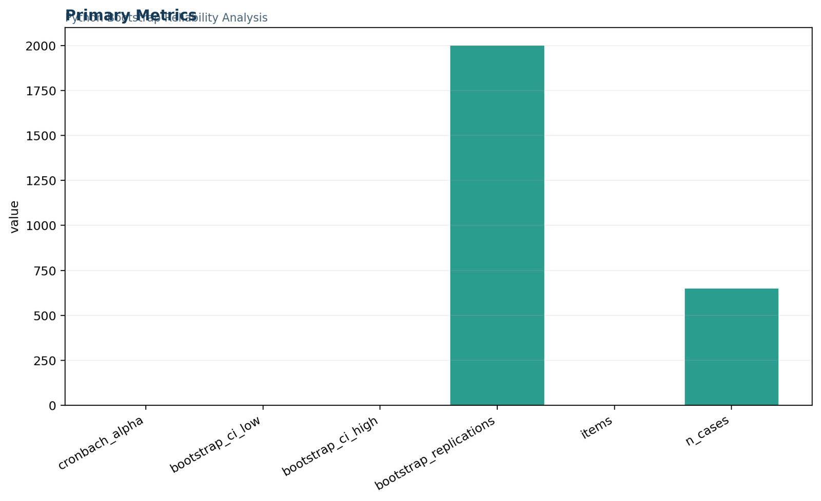
Primary metrics for reliability analysis in Python
The overview chart brings together the observed alpha, confidence limits, number of items, sample size, and bootstrap replication count. Because the metrics use very different numeric scales, the case count and replication count visually dominate the coefficient bars; exact labels are therefore essential.
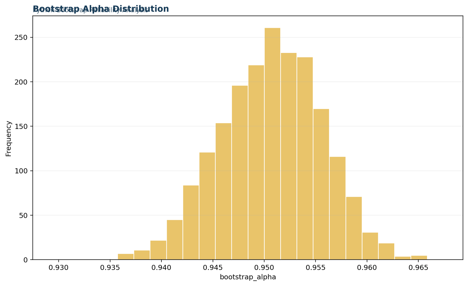
Bootstrap alpha distribution
The histogram concentrates near 0.951, with most replications falling inside the narrow percentile interval. The distribution is smooth and approximately centered on the observed coefficient.
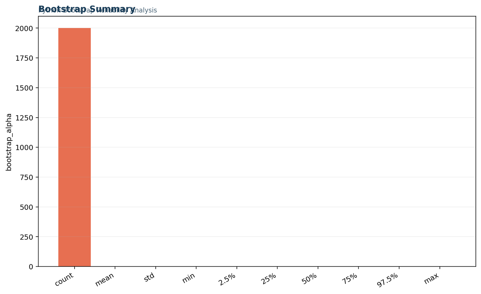
Bootstrap summary metrics
The summary chart records the bootstrap mean, median, spread, percentile limits, and replication count. Exact labels matter because 2,000 replications share an axis with coefficients close to one.
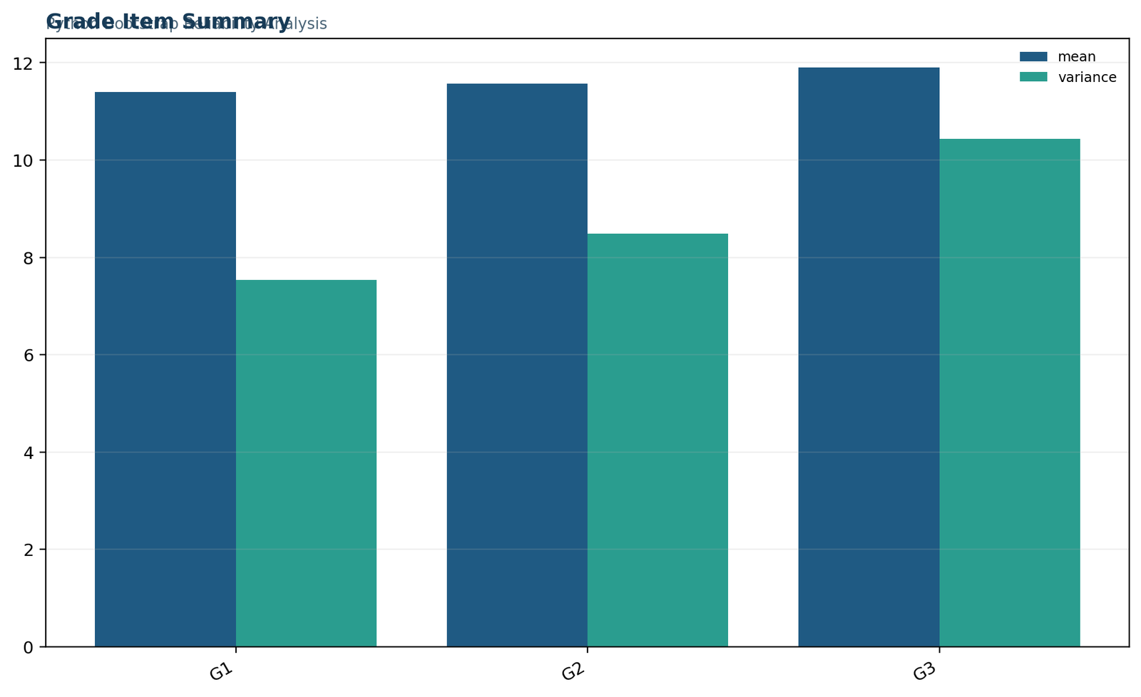
Grade-item means and variances
G1, G2, and G3 have similar means on the same grade scale, while variability rises from G1 to G3. The chart establishes the descriptive context for the covariance-based coefficient.
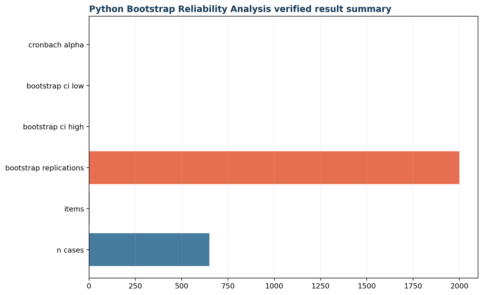
Verified result summary
The final chart restates the key coefficient, uncertainty limits, sample size, item count, and replication count as a compact verification panel.
How to read the coefficient bars
The alpha estimate of 0.950607 lies between the bootstrap limits of 0.940928 and 0.959780. Their close spacing communicates precision. The observed coefficient is near the center of the interval and almost identical to the bootstrap mean, which is reassuring for the stability of the result.
The lower limit is the most conservative value shown. Even that endpoint indicates that the three grade items remain highly consistent under plausible case resampling.
How to read the count bars
The chart also records three structural facts: the scale has three items, the analysis includes 649 cases, and the uncertainty estimate uses 2,000 bootstrap samples. These counts are not reliability coefficients and should not be compared by bar height with alpha.
Mixed-scale dashboards are useful summaries, but the viewer should rely on labels rather than visual length whenever coefficients and counts appear on one axis.
For public reporting, this chart works best as a compact audit trail. It shows that the result is not a single unsupported number: the coefficient is connected to a defined item set, a known sample size, and a documented uncertainty procedure. That combination is a central strength of the worked reliability analysis in Python.
Distribution shape
The histogram does not show a broad or multimodal pattern. Instead, the estimates cluster tightly around the observed value. The mean of 0.950666 and median of 0.950868 differ by only about 0.000202, so there is no practically important separation between the two centers.
The lower tail reaches 0.929378 and the upper tail reaches 0.967438, but those extrema are individual replications rather than interval endpoints. The central 95% interval excludes the most unusual 2.5% of estimates on each side.
Bootstrap spread
The bootstrap SD of 0.004977 is small relative to the coefficient. It measures how much alpha changes when student rows are repeatedly resampled from the observed empirical distribution. A small spread is expected when the sample is large and the inter-item relationships are strong.
The chart’s count bar should not be interpreted as a measure of precision by itself. More replications reduce Monte Carlo noise in the estimated percentiles, but they cannot compensate for an unrepresentative original sample or a poorly designed scale.
Together, the two charts make the uncertainty analysis transparent. The histogram answers “What did the resampled coefficients look like?” while the summary chart answers “Where were the key landmarks?” This pairing is more informative than reporting a confidence interval alone because readers can see whether the interval is supported by a stable, coherent distribution.
Why unequal variances are acceptable here
Raw alpha does not require all items to have identical variance. It uses each variance and covariance directly. Because all three grades use the same substantive scale, their variance differences are meaningful rather than artifacts of incompatible units.
The rise in variance toward G3 may reflect broader differentiation in final performance. It does not weaken reliability because G3 remains strongly correlated with G1 and especially G2.
What the verified summary adds
The verification chart repeats the result in one place so readers can reconcile the narrative, bootstrap output, and item description. Repetition of the exact values is valuable in a statistical report because transcription errors often occur when numbers are copied across sections.
The observed alpha, interval limits, case count, item count, and bootstrap count should match everywhere. Any mismatch should trigger a review of filtering, missing-data handling, random seed, or file version.
Item diagnostics: corrected item-total correlations and alpha if deleted
Item-level evidence shows whether each variable contributes meaningfully to the intended composite.
Item diagnostics extend reliability analysis in Python beyond the headline alpha. Corrected item-total correlation relates each item to the sum of the remaining items, preventing the item from correlating partly with itself. Alpha if deleted recalculates reliability after removing one item. These statistics identify unusual influence, but deletion decisions must remain substantive rather than mechanical.
| Item | Mean | Variance | Standard deviation | Interpretive note |
|---|---|---|---|---|
| G1 | 11.3991 | 7.5365 | 2.7453 | Lowest mean and smallest variance of the three grades. |
| G2 | 11.5701 | 8.4893 | 2.9136 | Intermediate mean and variability; strongest item-rest relationship. |
| G3 | 11.9060 | 10.4371 | 3.2307 | Highest mean and largest variance; still strongly aligned with earlier grades. |
| Item | Corrected item-rest correlation | Alpha if deleted | Interpretation |
|---|---|---|---|
| G1 | 0.862384 | 0.954888 | Very strong relationship with G2 + G3. Removing G1 raises alpha slightly, largely because G2 and G3 are exceptionally close. |
| G2 | 0.935171 | 0.898408 | Strongest item-rest relationship. Removing G2 substantially reduces consistency. |
| G3 | 0.904888 | 0.926723 | Very strong relationship with G1 + G2. Removing G3 reduces alpha. |
Why G1 should not be deleted automatically
Alpha rises from 0.950607 to 0.954888 when G1 is removed, an increase of only about 0.00428. That small change is not enough to justify deleting the first-period grade. A two-item coefficient for G2 and G3 benefits from their extremely high correlation, but it also narrows the time coverage of the composite.
If the intended score represents performance across the full academic sequence, retaining G1 improves content coverage even though the coefficient is fractionally lower. Reliability optimization is not the same as measurement quality optimization.
Why G2 is central to the scale
G2 has the strongest corrected relationship with the other grades. Removing it drops alpha to approximately 0.8984, the largest reduction among the three deletion checks. This pattern is consistent with G2 acting as a bridge between early and final performance.
The statistic does not prove that G2 is causally important. It shows that, within the covariance structure, G2 aligns especially well with the common score represented by G1 and G3.
Item-level evidence is essential when reliability analysis in Python is used to guide scale revision. Corrected item-rest correlations explain how each variable participates in reliability analysis in Python, while deletion coefficients show sensitivity. Neither statistic should turn reliability analysis in Python into an automatic item-removal algorithm.
Complete reliability analysis in Python workflow
A defensible workflow separates validation, estimation, uncertainty analysis, item review and reporting.
The following workflow describes how to conduct reliability analysis in Python without presenting a wall of code. It can be implemented with pandas and NumPy, supplemented by a statistical package for convenience. The crucial requirement is that every computational choice is explicit and checked.
Load and validate
Confirm row count, variable names, numeric conversion, score ranges, and duplicate cases.
Select and recode
Choose the intended items, reverse-score where needed, and define one missing-data rule.
Describe items
Calculate means, variances, standard deviations, ranges, and the inter-item matrix.
Estimate and diagnose
Calculate alpha, item-rest correlations, alpha if deleted, and complementary reliability measures.
Bootstrap and report
Resample complete rows, calculate the interval, verify outputs, and write an interpretation tied to the score purpose.
Data validation checklist
Computation checklist
Interpretation checklist
State the coefficient, item count, case count, interval, interval method, and resampling count. Describe the intended score rather than relying only on labels such as “good” or “excellent.” Discuss whether item diagnostics support retention and whether dimensionality has been examined.
Avoid causal language. Reliability concerns reproducibility or consistency of scores under a specified design; it does not show that one item causes another or that the scale predicts an outcome.
Output verification checklist
Reconcile every chart with the result table. Confirm that alpha equals 0.950607, the lower and upper percentile limits are 0.940928 and 0.959780, the case count is 649, and the bootstrap count is 2,000. Verify that item means and variances match the data used for the coefficient.
This final reconciliation is especially important when images, tables, and narrative text are created by different scripts or exported at different times.
Reproducible reliability analysis in Python separates validation, computation, and reporting so each stage can be checked. Saving the cleaned item matrix and result tables makes reliability analysis in Python easier to audit. Matching those files to every chart ensures that reliability analysis in Python remains consistent across publication formats.
Cronbach’s alpha compared with related reliability coefficients
Choose a coefficient that matches the measurement model, design and intended score interpretation.
| Method | Main question | Best use | Important distinction |
|---|---|---|---|
| Cronbach’s alpha | How consistently do items contribute to a common score? | Continuous or approximately continuous multi-item scales. | Strongest interpretation under tau-equivalence and approximate unidimensionality. |
| McDonald’s omega | How reliable is a factor-based composite when item loadings differ? | Scales with a defensible latent-variable model. | Requires a fitted factor model but relaxes equal-loading assumptions. |
| Split-half reliability | How consistent are two parts of a test? | Educational tests and internal replication checks. | Depends on how the items are split; the Spearman–Brown formula adjusts length. |
| Spearman–Brown coefficient | How does reliability change after test length changes? | Split-half correction and planning additional parallel items. | Assumes the added or removed items behave like the existing items. |
| Test-retest reliability | Are scores stable across occasions? | Temporal stability of a measure. | Can be reduced by true change, not only measurement error. |
| Intraclass correlation | How strongly do ratings or measurements agree? | Rater agreement, repeated measurements, and absolute agreement. | Several ICC models answer different consistency and agreement questions. |
| KR-20 | How consistent are dichotomously scored test items? | Correct/incorrect item sets. | Equivalent to alpha under binary scoring when computed from the same covariance structure. |
| Guttman coefficients | What lower-bound reliability estimates are supported by the score structure? | Alternative internal-consistency assessment. | Different lambda coefficients use different variance and split information. |
No single coefficient is universally best. A strong analysis chooses the statistic according to the data-generating process and intended claim. For the three continuous grade variables, raw alpha with a case bootstrap provides a clear internal-consistency summary. If the aim were absolute agreement among graders, an ICC would be more appropriate. If the aim were a latent academic-performance factor with unequal loadings, omega would provide a useful model-based companion.
Method choice determines what reliability analysis in Python can legitimately claim. Alpha-based reliability analysis in Python answers an internal-consistency question, whereas ICC, omega, and test-retest procedures address related but different designs. A strong reliability analysis in Python names those distinctions instead of treating all reliability coefficients as interchangeable.
Diagnostics, missing data, reverse scoring and common mistakes
A reliable coefficient requires a verified item matrix and a transparent analysis rule.
Missing-data inconsistency
Listwise deletion uses the same cases for every covariance and yields a coherent matrix. Pairwise deletion can use different case sets for different item pairs, sometimes producing a matrix that is difficult to interpret. Imputation introduces model assumptions. State the selected rule and resulting n.
Unreversed negative items
A negatively keyed item left in its original direction can create negative correlations and a low or even negative alpha. Reverse scoring must use the correct scale endpoints, and the recoded variable should be checked against the original.
Mixing incompatible scales
Raw alpha is sensitive to item units. Combining a 0-to-100 score with a 1-to-5 item can let the high-variance variable dominate. Standardization may be appropriate, but a conceptual review is required first.
Redundancy mistaken for quality
Very similar items can inflate alpha while adding little information. Review wording and content overlap when correlations approach one or the scale feels repetitive.
Ignoring multidimensionality
A high overall alpha can emerge from several correlated subscales. Factor analysis, theory, and subscale-specific reliability are needed before treating the total as one dimension.
Alpha fishing
Repeatedly deleting items until alpha rises capitalizes on sample-specific noise. Item retention should be guided by theory, validity, and cross-sample confirmation.
Negative alpha
A negative coefficient means the average covariance is negative or the item coding is severely inconsistent. Common causes are unreversed items, data-entry errors, mixed constructs with opposite directions, or selecting variables that should not form a scale. It is not a low but usable reliability estimate; it is a diagnostic alarm.
Alpha greater than one
A correctly computed alpha from a valid positive-semidefinite covariance matrix should not exceed one. Values above one usually indicate a formula error, inconsistent variance conventions, corrupted covariance input, or numerical issues. Recalculate from the cleaned item matrix and verify the total-score variance.
For the grade example, the main diagnostics are favorable: all pairwise correlations are strong and positive, every corrected item-rest correlation is high, no item has trivial variance, and the bootstrap distribution is narrow. The only caution is interpretive: three repeated grades are temporally ordered measurements, so a high alpha should not erase meaningful change across periods.
Quality control protects reliability analysis in Python from silent coding and selection errors. Negative covariances, impossible values, duplicated rows, and mixed scoring directions can invalidate reliability analysis in Python even when the software runs successfully. Reviewing these conditions makes reliability analysis in Python a defensible analytical process rather than a button-click result.
How to report reliability analysis in Python in APA style
Report the coefficient, item set, sample size, uncertainty method and interpretation in one coherent result statement.
APA-style result paragraph
A reliability analysis was conducted in Python for the three grade indicators G1, G2, and G3 using 649 complete student records. The scale demonstrated excellent internal consistency, Cronbach’s α = .951. A nonparametric case-resampling bootstrap with 2,000 replications produced a percentile 95% confidence interval from .941 to .960, with a bootstrap mean of .951 and bootstrap SD of .005. Corrected item-rest correlations ranged from .862 to .935. These results indicate that the grade measurements share substantial common variation and support a highly consistent composite score, although the coefficient alone does not establish unidimensionality or validity.
Expanded methods statement
Reliability was evaluated using raw covariance-based Cronbach’s alpha. G1, G2, and G3 were retained on their original common grade scale. Complete student rows were used, resulting in n = 649. Sampling uncertainty was estimated by resampling complete rows with replacement 2,000 times and taking the 2.5th and 97.5th percentiles of the bootstrap alpha distribution as the 95% confidence limits.
Expanded interpretation statement
The coefficient and its narrow interval provide strong evidence of stable internal consistency in this sample. G2 showed the strongest corrected association with the remaining grades. Deleting G1 increased alpha only slightly and would reduce coverage of the full grade sequence, so item deletion is not supported by reliability optimization alone.
| Reporting element | What to include | Worked example |
|---|---|---|
| Scale definition | Names and interpretation of included items | G1, G2, and G3 as repeated academic-performance indicators |
| Estimator | Raw or standardized alpha and software environment | Raw Cronbach’s alpha in Python |
| Sample | Final case count and missing-data rule | 649 complete rows |
| Point estimate | Coefficient with sensible rounding | α = .951 |
| Uncertainty | Interval type, level, and replication count | Percentile bootstrap 95% CI [.941, .960], 2,000 resamples |
| Item evidence | Item-rest range and influential deletion results | Corrected item-rest r = .862 to .935 |
| Boundary statement | What the result does not establish | Does not by itself prove validity or unidimensionality |
Clear reporting allows another analyst to reconstruct reliability analysis in Python from the stated design. The coefficient, confidence interval, item count, case count, bootstrap method, and item diagnostics are all part of reliability analysis in Python. Including interpretation limits ensures that reliability analysis in Python is not presented as evidence for claims it cannot support.
Reliability analysis in Python PDF, workbook and guide downloads
Open the verified Python report and worked files used to audit the published result.
Worked Excel analysisCalculation audit and tabular review of the reliability results.Open workbook →
Cronbach’s alpha guideFormula, interpretation, assumptions, and common reporting issues.Read guide →
McDonald’s omega guideFactor-model reliability when item loadings are not assumed equal.Read guide →
The downloadable files extend reliability analysis in Python from a narrative into a verifiable record. The report preserves exact output from reliability analysis in Python, and the workbook supports independent checking. Keeping those resources beside the article makes future reliability analysis in Python updates easier to reconcile with the published result.
Reliability analysis in Python verification references
Technical sources and internal guides used to check the coefficient, bootstrap design and item diagnostics.
The formulas and workflow in this reliability analysis in Python were checked against established covariance-based reliability definitions and the documented behavior of the Python tools used for data handling and resampling. The published numbers were also reconciled across the report, workbook, tables and five chart files.
Python numerical stack
pandas is used for column selection, numeric validation and complete-case handling. NumPy supports reproducible row resampling and matrix calculations. The coefficient is calculated directly from sample item variances and total-score variance so every step remains visible.
Reliability definitions
The interpretation follows the covariance-based definition of raw Cronbach’s alpha and distinguishes internal consistency from dimensionality and validity. See the internal Cronbach’s alpha guide and McDonald’s omega guide.
Uncertainty and item checks
The percentile interval is based on 2,000 complete-row bootstrap samples. Item contribution is reviewed with corrected item-total correlations and alpha if deleted. Continue with corrected item-total correlation and confidence intervals.
Reliability analysis in Python FAQs
Answers to the most common questions about Cronbach’s alpha, bootstrap intervals and item diagnostics.
What is reliability analysis in Python?
It is a reproducible workflow for evaluating score consistency with Python data tools. A complete analysis includes item validation, descriptive statistics, inter-item relationships, a coefficient such as Cronbach’s alpha, uncertainty, item diagnostics, and a written interpretation.
What was Cronbach’s alpha in the worked example?
Raw Cronbach’s alpha for G1, G2, and G3 was 0.950607 using 649 complete student records.
What does an alpha of 0.951 mean?
It indicates that the three grade measurements have excellent internal consistency in this sample. Students’ relative performance is strongly preserved across the three grade periods.
Does alpha of 0.951 prove the scale is valid?
No. Alpha describes consistency, not whether the score measures the intended construct or supports a particular decision. Validity requires additional substantive and empirical evidence.
How many bootstrap samples were used?
The analysis used 2,000 case-resampling bootstrap replications. Each replication sampled complete student rows with replacement and recalculated alpha.
What was the bootstrap confidence interval?
The percentile 95% bootstrap interval extended from 0.940928 to 0.959780. The entire interval indicates high consistency.
Why bootstrap Cronbach’s alpha?
Bootstrapping estimates sampling uncertainty without relying entirely on a closed-form normal-theory interval. It also reveals the shape, center, and spread of plausible coefficients under repeated case sampling.
Should bootstrap sampling be done by row or by item?
By row. Each row contains the related item scores for one case. Sampling columns independently would destroy the covariance structure that alpha measures.
What is the difference between raw and standardized alpha?
Raw alpha uses the covariance matrix and retains item variance differences. Standardized alpha uses the correlation matrix and places items on equal variance scales. Raw alpha is natural when items share meaningful units.
Does Cronbach’s alpha require normal data?
The coefficient can be calculated without normality. However, distributional assumptions can affect some confidence intervals and inferential procedures. Bootstrap intervals are useful when normal-theory assumptions are doubtful.
Does high alpha prove unidimensionality?
No. Several correlated dimensions or redundant items can produce a high coefficient. Dimensionality should be evaluated with theory and factor-analytic evidence.
Can alpha be high with only three items?
Yes, but the average inter-item relationships must be very strong. In this example, pairwise correlations range from approximately 0.826 to 0.919.
Which grade item was most strongly related to the scale?
G2 had the largest corrected item-rest correlation, approximately 0.935. It aligned particularly strongly with the combined information in G1 and G3.
Should G1 be deleted because alpha rises slightly?
No automatic deletion is justified. Removing G1 raises alpha only from 0.950607 to 0.954888 and reduces coverage of the full grade sequence. Content and purpose matter more than maximizing the coefficient.
What is alpha if G2 is deleted?
Alpha falls to approximately 0.898408, showing that G2 contributes strongly to the consistency of the three-grade composite.
What is alpha if G3 is deleted?
Alpha becomes approximately 0.926723. The remaining G1 and G2 pair is still highly consistent, but the coefficient is lower than the full three-item result.
What corrected item-total correlation is acceptable?
Rules such as 0.30 are only rough screening guides. Interpretation should consider construct breadth, item count, sample, and purpose. The present values above 0.86 are exceptionally strong.
Can Cronbach’s alpha be negative?
Yes, when average item covariance is negative. This usually signals reverse-coding errors, incompatible items, data problems, or a scale that should not be combined.
Can Cronbach’s alpha exceed one?
Not in a valid calculation from a proper covariance matrix. A value above one indicates an implementation, data, or numerical error that should be investigated.
How does alpha differ from an ICC?
Alpha usually addresses internal consistency among items. An ICC addresses reliability or agreement among measurements or raters under a specified variance-components model. The correct ICC form depends on the design and whether consistency or absolute agreement is required.
When should McDonald’s omega be reported?
Omega is useful when a factor model is defensible and item loadings differ. Reporting omega beside alpha provides a more flexible view of composite reliability.
How should missing data be handled?
Choose a defensible rule before estimation and report it. Complete-case analysis, pairwise covariance, and imputation can produce different results. The worked example uses complete cases for all three selected grades.
What random seed should be used for bootstrapping?
Any fixed, documented seed is acceptable. The purpose is reproducibility, not selecting a seed that produces a preferred interval.
Are 2,000 bootstrap replications enough?
Two thousand replications are generally adequate for a stable teaching and reporting example. More replications can reduce Monte Carlo noise in percentile endpoints, especially when very precise tail estimates are needed.
Can reliability differ across groups?
Yes. A scale can be more or less reliable across schools, languages, age groups, or other populations. Group-specific coefficients and intervals should be evaluated when comparability is important.
Why can means change while alpha remains high?
Alpha reflects covariance and relative ordering, not equality of means. Students can improve on average while maintaining similar rank positions, producing both mean change and high consistency.
What is the main conclusion from this reliability analysis in Python?
G1, G2, and G3 form a highly consistent three-item composite in the 649-student sample. The observed alpha is 0.950607, and the bootstrap evidence shows that the estimate is precise and stable, while validity and dimensionality still require separate evidence.
The questions below summarize the decisions that most often affect reliability analysis in Python. They reinforce that reliability analysis in Python includes score design, uncertainty, diagnostics, and interpretation—not only alpha. Used as a final checklist, they help readers apply reliability analysis in Python without repeating common measurement errors.
Related reliability and measurement guides
Continue with the coefficients, diagnostics and interpretation concepts most closely connected to reliability analysis in Python.