
Limits of Agreement: 7 Essential Steps, Formula, Confidence Intervals and Worked Example
The limits of agreement method estimates how far two paired measurements can differ for an individual. This complete guide explains the Bland–Altman limits of agreement formula, confidence intervals for the mean bias and both limits, assumptions, interpretation, a verified G3 minus G2 example, and reproducible workflows in Python, R, SPSS and Excel.
G3 is about 0.34 points higher than G2 on average, but individual differences are much wider.
For 649 complete G2–G3 pairs, the difference was defined as G3 − G2. The mean difference, or bias, was 0.3359 grade points, with a 95% confidence interval from 0.2374 to 0.4344. The difference standard deviation was 1.2782, producing classical 95% limits of agreement from −2.1695 to 2.8413.
The average bias is statistically different from zero, t(648) = 6.695, p < .001. That test addresses the average paired difference only. The limits of agreement address the more important individual-level question: how different might G2 and G3 be for one student?
What do limits of agreement measure?
A direct estimate of individual disagreement, not merely association or average change.
Limits of agreement describe the interval within which most differences between two measurements on the same unit are expected to fall. They are usually presented with a Bland–Altman plot, but the numerical estimates and their uncertainty remain useful even when the immediate task is a table, report or software cross-check.
The individual-level question
Suppose the same student has a second-period grade G2 and a final grade G3. A correlation can show whether high G2 scores tend to accompany high G3 scores, but it cannot show whether the two values are close enough to be used interchangeably. The limits of agreement method works with the paired difference for every student.
In this analysis the signed difference is G3 − G2. A positive difference means G3 is higher; a negative difference means G3 is lower. The mean of these differences estimates systematic bias. Their standard deviation estimates the ordinary person-to-person variation around that bias.
What the limits do not prove
The interval does not prove that two methods, occasions or raters are interchangeable. It does not replace an externally justified acceptable-difference margin. It also does not test whether the two measurements have the same correlation, variance or reliability coefficient.
Use the Bland–Altman plot guide when the visual pattern is the main focus, intraclass correlation when a reliability coefficient is needed, and a paired-samples analysis when the research question is limited to the average change.
Bias
The mean paired difference. It estimates systematic direction and size of average disagreement.
Random disagreement
The standard deviation of paired differences. It determines how widely individual differences vary around the bias.
Agreement interval
Bias ± 1.96 difference SD under the classical normal-difference model. It targets approximately 95% of individual differences.
When should limits of agreement be used?
Use the decision logic before calculating a bias, p-value or plot.
Use limits of agreement when every observational unit has two measurements that are meaningfully paired and the scientific question is how closely those measurements agree. The method is commonly applied to two devices, two raters, two laboratory assays, two occasions, or two scoring procedures.
Two paired values?
Each student, patient, device or specimen must contribute one value from each method or occasion.
Same scale?
The two measurements should use the same units or a defensible transformation to a common scale.
Individual agreement?
The question must concern the size of within-pair differences, not only the average difference.
Acceptable margin?
Define what difference would be practically tolerable before judging the limits.
Stable pattern?
Check whether bias or spread changes across the measurement magnitude.
Appropriate applications
Situations requiring another design
Limits of agreement assumptions: six conditions to check
The method is simple to calculate but not assumption-free.
The classical limits of agreement assumptions concern the paired design, independence between units, the distribution of differences, and stability of the bias and spread across the measurement range. These conditions are more relevant than testing each raw measurement for normality.
Correct pairing
G2 and G3 must belong to the same student. A single row mismatch can create artificial disagreement and distort every result.
Independent units
Pairs should be independent across students. Clustered observations within classes, schools, families or devices may need multilevel agreement methods.
Meaningful difference
Subtraction must make scientific sense. Both measurements must use the same scale, units and direction.
Difference distribution
The classical 1.96 multiplier assumes the paired differences are approximately normal, especially in their tails.
Constant bias
The average difference should not change materially as the pair mean increases. A trend suggests proportional bias.
Constant spread
The variability of differences should be reasonably similar across low and high measurement magnitudes.
What should be normal?
Normality concerns the paired differences, not G2 and G3 separately. Testing the raw variables can answer the wrong question. Review the normal distribution, the Shapiro–Wilk test, and histogram interpretation when documenting this assumption.
With n = 649, formal normality tests have high power, but the current deviation is not a trivial large-sample rejection: the skewness, kurtosis, minimum of −9 and visible tail pattern are substantively strong.
What can be done?
When non-normality arises from a meaningful multiplicative structure, a log transformation may stabilize spread. When the outcome is discrete and bounded, transformation may not solve the problem. Alternatives include empirical quantile limits, robust limits, bootstrap confidence intervals, stratified analysis, or a regression-based method.
Outliers should be investigated through data lineage and subject-matter review, not automatically deleted. See outlier detection for a structured workflow.
Questions, hypotheses and decisions for limits of agreement
Separate average bias, individual disagreement and practical acceptability.
Limits of agreement are primarily an estimation method. The central deliverables are the bias, lower limit, upper limit and confidence intervals. A hypothesis test for zero mean bias can be added, but it does not test overall agreement.
Questions answered by the analysis
Formal bias hypothesis
The population mean difference is zero.
The population mean difference is not zero.
For G3 − G2, the observed result is t(648) = 6.695, p < .001. The mean bias is therefore statistically different from zero. This conclusion is separate from the width of the limits.
Agreement is not the null hypothesis
Failing to reject zero bias would not prove good agreement. Two measurements can have no average bias and still differ widely for individuals. Likewise, a small statistically significant bias can coexist with narrow and practically acceptable limits when the sample is large.
The practical question should be written as an interval comparison: are both estimated limits, and preferably their confidence intervals, contained within the prespecified acceptable region?
Equivalence requires margins
A formal equivalence analysis must define lower and upper acceptable boundaries before the data are examined. The confidence interval for bias can then be compared with a mean-bias equivalence margin, while the confidence intervals for the limits can be compared with individual-difference margins.
Do not convert a nonsignificant p-value into evidence of equivalence. See confidence intervals and statistical power for the logic behind precision-based decisions.
Worked-analysis conclusion
The source workbook states a null hypothesis that the G2–G3 bias is zero and the population agreement interval is acceptably narrow. The first component is testable from the paired differences and is rejected. The second component cannot be decided statistically without a supplied definition of “acceptably narrow.” The correct report therefore gives the exact limits and asks readers to compare them with the practical tolerance relevant to the grade scale.
Limits of agreement formula and confidence intervals
A complete calculation from paired differences to uncertainty around both boundaries.
The classical limits of agreement formula begins with one signed difference per pair. The choice of direction must remain unchanged throughout the analysis because reversing the subtraction reverses the bias and swaps the signs of both limits.
Step 1: calculate each paired difference and pair mean
A positive value means the final grade is higher. A negative value means it is lower.
The pair mean is used on the horizontal axis of a Bland–Altman plot and in proportional-bias diagnostics.
Step 2: estimate bias and difference variation
The current bias is 0.335901 grade points.
The current difference standard deviation is 1.278245.
Step 3: calculate the classical 95% limits
0.335901 − 1.96(1.278245) = −2.169458.
0.335901 + 1.96(1.278245) = 2.841261.
Confidence interval for bias
With n = 649, SE(d̄) = 0.0501755 and t = 1.96363. The 95% confidence interval is 0.237375 to 0.434428.
Confidence intervals for the limits
The standard error for each limit is 0.0857952. The lower-limit CI is approximately −2.337928 to −2.000988, and the upper-limit CI is approximately 2.672791 to 3.009731.
| Quantity | Formula | Current result | Interpretation |
|---|---|---|---|
| Bias | d̄ | 0.335901 | Average G3 − G2 difference. |
| Difference SD | sd | 1.278245 | Variation of individual paired differences. |
| Lower limit | d̄ − 1.96sd | −2.169458 | Lower classical boundary for about 95% of differences. |
| Upper limit | d̄ + 1.96sd | 2.841261 | Upper classical boundary for about 95% of differences. |
| Bias CI | d̄ ± tSE(d̄) | 0.237375 to 0.434428 | Precision of the estimated average bias. |
| Limit SE | sd√[1/n + 1.96²/[2(n−1)]] | 0.085795 | Sampling uncertainty of either limit. |
Limits of agreement worked example: G3 versus G2
A complete paired-grade calculation with transparent variable coding.
This worked limits of agreement example uses G2 and G3 from 649 student records. G2 is the second-period grade and G3 is the final grade. The example treats them as two paired occasions on the same numerical grading scale.
Variables used
| Role | Variable | Definition |
|---|---|---|
| First measurement | G2 | Second-period grade. |
| Second measurement | G3 | Final grade. |
| Difference | G3 − G2 | Positive means improvement; negative means decline. |
| Magnitude | (G2 + G3)/2 | Average grade used to evaluate proportional bias. |
| Unit | Student | One independent pair per student. |
Data preparation rules
Observed difference frequencies
The discrete grade scale produces only 13 distinct differences. Exact agreement occurred for 287 students (44.2%). G3 exceeded G2 by one point for 234 students (36.1%), while G3 was one point lower for 56 students (8.6%). These three values alone account for 577 of the 649 pairs.
| G3 − G2 | Frequency | Percent | Meaning |
|---|---|---|---|
| −9 to −3 | 13 | 2.0% | Large declines, including the long negative tail. |
| −2 | 3 | 0.5% | Two-point decline. |
| −1 | 56 | 8.6% | One-point decline. |
| 0 | 287 | 44.2% | Exact numerical agreement. |
| +1 | 234 | 36.1% | One-point increase. |
| +2 | 47 | 7.2% | Two-point increase. |
| +3 to +6 | 9 | 1.4% | Larger increases. |
Limits of agreement results and exact interpretation
Verified estimates, confidence intervals, coverage and diagnostics.
The exact limits of agreement results combine estimation, a separate bias test, diagnostics and empirical coverage. Every result below is cross-checked across the Excel workbook and the Python, R and SPSS outputs.
Primary agreement result
Classical 95% limits
Under the classical model, most individual G3 − G2 differences are expected between about 2.17 points lower and 2.84 points higher. The interval is asymmetric around zero because the average bias is positive.
Calculation audit
| Result component | Estimate | 95% confidence interval | Interpretation |
|---|---|---|---|
| Mean bias | 0.335901 | 0.237375 to 0.434428 | G3 is higher than G2 by about one-third of a point on average. |
| Lower agreement limit | −2.169458 | −2.337928 to −2.000988 | Lower boundary for individual G3 − G2 differences. |
| Upper agreement limit | 2.841261 | 2.672791 to 3.009731 | Upper boundary for individual G3 − G2 differences. |
| Bias test | t = 6.695 | df = 648, p < .001 | The average difference is statistically different from zero. |
| Mean–difference relation | r = 0.253 | p < .001 | Differences become more positive as the average grade increases. |
Empirical coverage
Twenty-two of the 649 observed differences fall outside the estimated classical limits. Therefore, 627 pairs (96.61%) are inside and 3.39% are outside. This sample proportion is close to, but not required to equal, 95% because the boundaries are estimated from the same data and the differences are discrete and non-normal.
Coverage alone is not a sufficient diagnostic. A model can include approximately 95% of observations while still showing proportional bias, heteroscedasticity or clinically unacceptable width.
Distribution summary
The difference median is 0, the IQR is 1, the minimum is −9, and the maximum is 6. Skewness is −3.031 and kurtosis is 19.487. These values confirm a central spike with unusually heavy tails.
Use skewness, kurtosis, range, and interquartile range together. No single descriptive measure fully represents the agreement pattern.
Limits of agreement in Python: complete calculation and charts
A transparent calculation with exact confidence intervals and diagnostics.
A reproducible limits of agreement Python workflow should calculate the paired differences, bias, sample difference SD, classical limits, confidence intervals, empirical coverage and diagnostics. The code below keeps all formulas visible rather than relying on a single black-box function.
import numpy as np
import pandas as pd
from scipy import statsdf = pd.read_csv("dataset.csv")
pairs = df[["G2", "G3"]].dropna().copy()
pairs["mean_pair"] = pairs[["G2", "G3"]].mean(axis=1)
pairs["difference"] = pairs["G3"] - pairs["G2"]
n = len(pairs)
bias = pairs["difference"].mean()
sd_diff = pairs["difference"].std(ddof=1)
loa_low = bias - 1.96 * sd_diff
loa_high = bias + 1.96 * sd_diff
tcrit = stats.t.ppf(0.975, n - 1)
se_bias = sd_diff / np.sqrt(n)
se_limit = sd_diff * np.sqrt(1/n + 1.96**2/(2*(n-1)))
bias_ci = (bias - tcrit*se_bias, bias + tcrit*se_bias)
low_ci = (loa_low - tcrit*se_limit, loa_low + tcrit*se_limit)
high_ci = (loa_high - tcrit*se_limit, loa_high + tcrit*se_limit)
outside = ((pairs["difference"] < loa_low) |
(pairs["difference"] > loa_high)).sum()
Python Primary metrics for limits of agreement
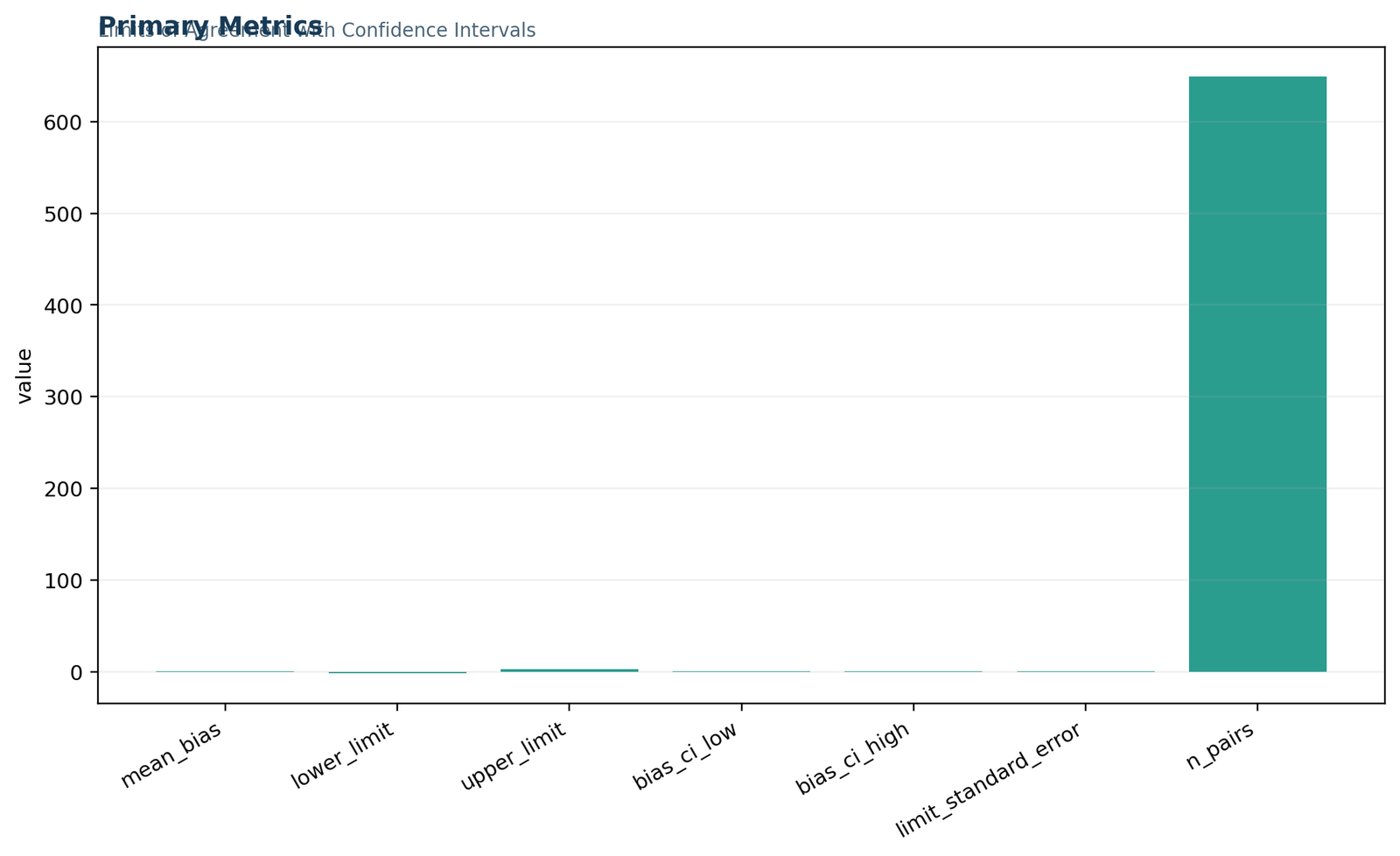
The primary metrics panel summarizes all 649 pairs, the G3 minus G2 mean bias of 0.3359, the difference standard deviation of 1.2782, and the classical 95% limits from −2.1695 to 2.8413. Read this first because every later table and confidence interval must reconcile to these values.
Python Paired differences for G2 and G3
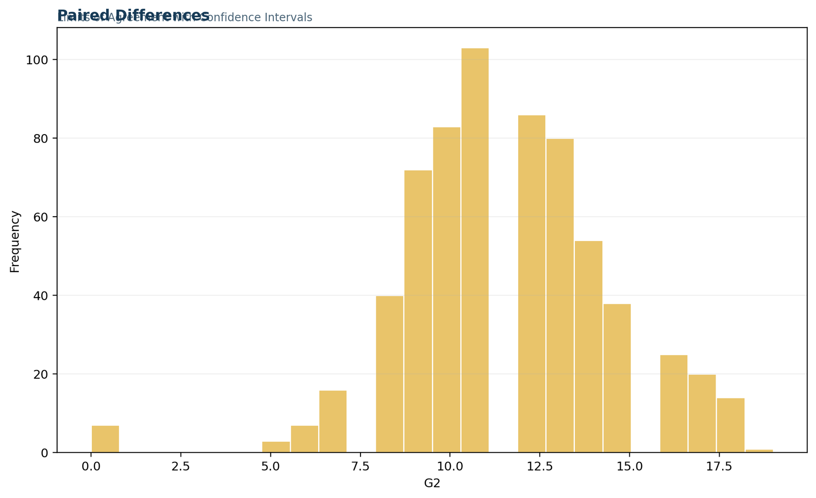
The paired-difference display keeps the direction G3 − G2 visible. Positive values mean the final grade is higher than the second-period grade, negative values mean it is lower, and zero represents exact agreement. Most observations are concentrated at −1, 0, or +1, but a small number of large negative differences create the long left tail.
Python Agreement limits with confidence intervals
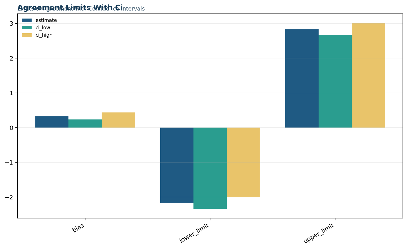
This figure separates the estimated bias from the lower and upper agreement boundaries and adds uncertainty around each estimate. The bias confidence interval is 0.2374 to 0.4344; the approximate confidence interval for the lower limit is −2.3379 to −2.0010, and the approximate confidence interval for the upper limit is 2.6728 to 3.0097.
Python Difference distribution summary
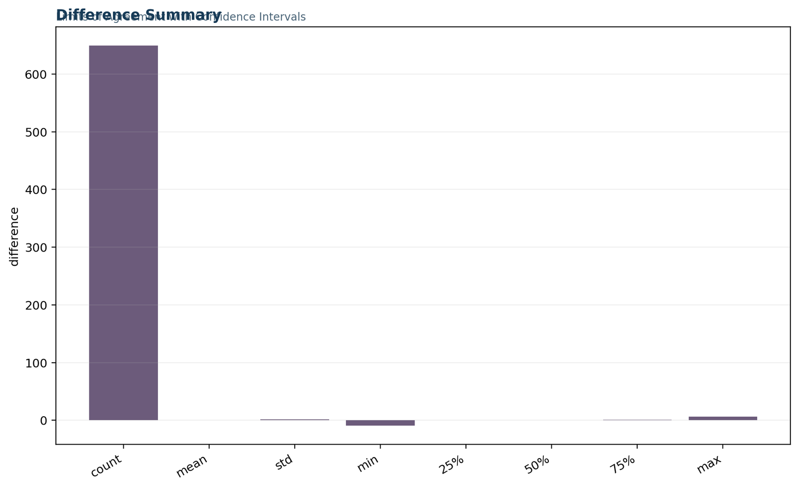
The distribution summary shows a median difference of 0, an interquartile range of 1, a minimum of −9, and a maximum of 6. The strong negative skew and heavy tails explain why the normality diagnostics require explicit discussion instead of a routine statement that assumptions were satisfied.
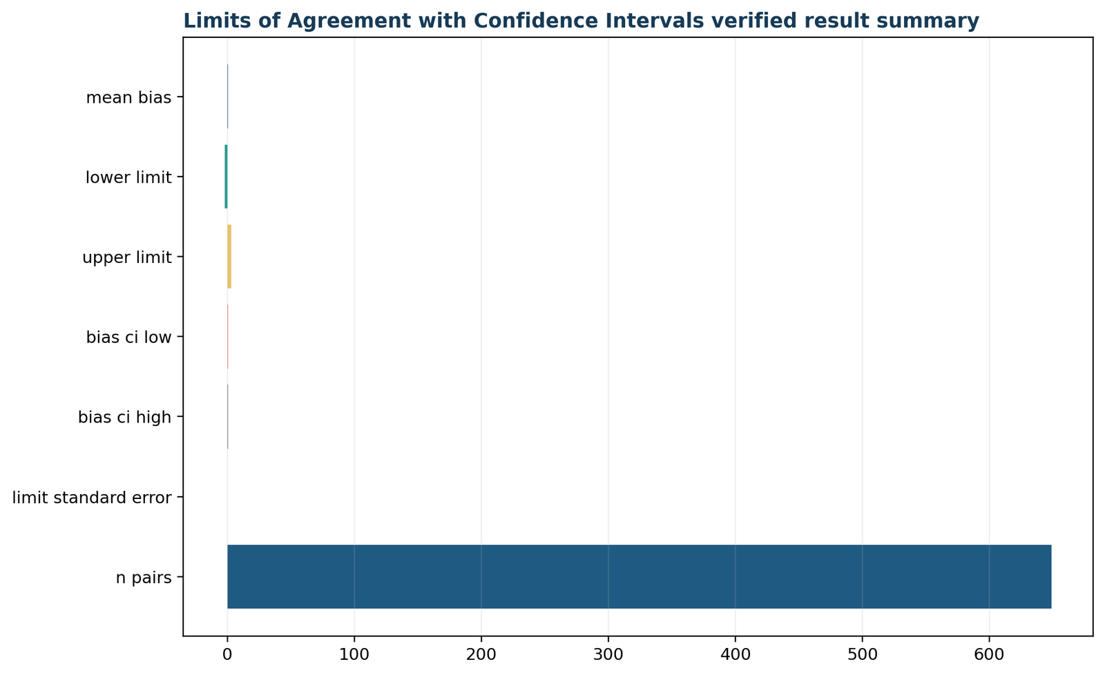
Python Verified limits of agreement result summary
The verified result card reconciles Python, R, SPSS, and Excel. The independent implementations agree on n = 649, bias = 0.335901, lower limit = −2.169458, upper limit = 2.841261, and the standard error of each limit = 0.085795.
Python validation checks
Python diagnostics
Calculate the correlation between pair mean and difference, inspect a scatterplot, summarize the difference distribution, and review outlying rows. In this dataset, r = 0.253 with p < .001, so the difference is not completely independent of measurement magnitude.
A regression-based Bland–Altman extension may be preferable when that trend is scientifically meaningful.
Limits of agreement in R: formulas, confidence intervals and charts
Base R reproduces the complete verified analysis without hidden defaults.
The limits of agreement in R can be reproduced with base functions. The workflow below deliberately calculates every component so the R output can be reconciled with Python, SPSS and Excel.
df <- read.csv("dataset.csv")
d <- na.omit(df[c("G2", "G3")])d$mean_pair <- rowMeans(d[c("G2", "G3")])
d$difference <- d$G3 - d$G2
n <- nrow(d)
bias <- mean(d$difference)
sd_diff <- sd(d$difference)
loa_low <- bias - 1.96 * sd_diff
loa_high <- bias + 1.96 * sd_diff
tcrit <- qt(.975, df = n - 1)
se_bias <- sd_diff / sqrt(n)
se_limit <- sd_diff * sqrt(1/n + 1.96^2/(2*(n-1)))
bias_ci <- bias + c(-1, 1) * tcrit * se_bias
low_ci <- loa_low + c(-1, 1) * tcrit * se_limit
high_ci <- loa_high + c(-1, 1) * tcrit * se_limit
R Primary metrics for limits of agreement
The primary metrics panel summarizes all 649 pairs, the G3 minus G2 mean bias of 0.3359, the difference standard deviation of 1.2782, and the classical 95% limits from −2.1695 to 2.8413. Read this first because every later table and confidence interval must reconcile to these values.
R Paired differences for G2 and G3
The paired-difference display keeps the direction G3 − G2 visible. Positive values mean the final grade is higher than the second-period grade, negative values mean it is lower, and zero represents exact agreement. Most observations are concentrated at −1, 0, or +1, but a small number of large negative differences create the long left tail.
R Agreement limits with confidence intervals
This figure separates the estimated bias from the lower and upper agreement boundaries and adds uncertainty around each estimate. The bias confidence interval is 0.2374 to 0.4344; the approximate confidence interval for the lower limit is −2.3379 to −2.0010, and the approximate confidence interval for the upper limit is 2.6728 to 3.0097.
R Difference distribution summary
The distribution summary shows a median difference of 0, an interquartile range of 1, a minimum of −9, and a maximum of 6. The strong negative skew and heavy tails explain why the normality diagnostics require explicit discussion instead of a routine statement that assumptions were satisfied.
R Verified limits of agreement result summary
The verified result card reconciles Python, R, SPSS, and Excel. The independent implementations agree on n = 649, bias = 0.335901, lower limit = −2.169458, upper limit = 2.841261, and the standard error of each limit = 0.085795.
R numerical reconciliation
The R results should match the verified ledger to ordinary floating-point precision. The Excel workbook reports absolute differences of zero for the bias, bias confidence limits, limit standard error and n; the lower and upper limits differ only by about 9.8 × 10⁻¹⁵ because of binary floating-point representation.
R diagnostic extensions
Use cor.test(d$mean_pair, d$difference) for the mean–difference association, shapiro.test() only with awareness of its sample-size limitations, and graphical diagnostics for the full pattern. For discrete grades, empirical quantiles and bootstrap procedures can be added as sensitivity analyses.
Limits of agreement in SPSS: workflow and verified output
Transform the paired values, estimate bias and examine the agreement assumptions.
The limits of agreement SPSS workflow begins by creating the pair mean and signed difference. SPSS can then provide descriptives, a bias test, a mean–difference correlation, a scatterplot, a histogram and Q–Q diagnostics. The classical limits and confidence intervals are calculated from the verified formulas.
SPSS transformations and summaries
COMPUTE loa_difference = G3 - G2.
COMPUTE loa_mean = (G2 + G3) / 2.
EXECUTE.DESCRIPTIVES VARIABLES=loa_difference loa_mean
/STATISTICS=MEAN STDDEV VARIANCE MIN MAX.
T-TEST /TESTVAL=0
/VARIABLES=loa_difference
/CRITERIA=CI(.95).
SPSS diagnostics
CORRELATIONS
/VARIABLES=loa_mean loa_difference
/PRINT=TWOTAIL NOSIG
/MISSING=PAIRWISE.GRAPH
/SCATTERPLOT(BIVAR)=loa_mean WITH loa_difference.
EXAMINE VARIABLES=loa_difference
/PLOT=HISTOGRAM NPPLOT
/STATISTICS=DESCRIPTIVES.
| SPSS output | Verified value | Meaning |
|---|---|---|
| Difference mean | 0.3359 | Average G3 − G2 bias. |
| Difference SD | 1.27824 | Variation used to construct the limits. |
| One-sample t | 6.695, df = 648, p < .001 | Bias differs from zero. |
| Bias CI | 0.2374 to 0.4344 | Precision of the mean difference. |
| Mean–difference correlation | 0.253, p < .001 | Evidence of magnitude-related bias. |
| Shapiro–Wilk | 0.685, p < .001 | Strong departure from normal differences. |
The complete uploaded SPSS report contains 649 rows, the G3 − G2 difference, pair mean, descriptives, one-sample test, correlation and normality diagnostics. Its final verification ledger reports the same bias and limits as the other software implementations.
Limits of agreement in Excel: worked formulas and audit trail
A transparent workbook that reproduces every verified metric.
The worked limits of agreement Excel workbook is formula-driven and separates source data, row calculations, final metrics, diagnostics and reporting. It is designed as an audit trail rather than a one-cell answer.
Recommended workbook structure
| Sheet | Purpose | Key content |
|---|---|---|
| Guide | Method documentation | Design, variables, formula, alpha and reproducibility notes. |
| Data_Input | Original paired values | Unchanged G2 and G3 columns. |
| Working | Row-level calculations | Pair mean, difference and squared difference. |
| Calculations | Metric ledger | n, bias, lower limit, upper limit, CIs and verified references. |
| Diagnostics | Quality checks | Assumptions, row count and scope. |
| Reporting | Final comparison | Workbook results, verified results and absolute differences. |
Core Excel formulas
Difference:       =B2-A2

Pair mean:        =AVERAGE(A2:B2)

Bias:             =AVERAGE(DifferenceRange)

Difference SD:    =STDEV.S(DifferenceRange)

Lower limit:      =Bias-1.96*DifferenceSD

Upper limit:      =Bias+1.96*DifferenceSD

SE bias:          =DifferenceSD/SQRT(n)

SE limit:         =DifferenceSD*SQRT(1/n+1.96^2/(2*(n-1)))
Confidence interval formulas
t critical:       =T.INV.2T(0.05,n-1)

Bias CI low:      =Bias-tCritical*SEBias

Bias CI high:     =Bias+tCritical*SEBias

Lower LoA CI low: =LowerLimit-tCritical*SELimit

Lower LoA CI high:=LowerLimit+tCritical*SELimit

Upper LoA CI low: =UpperLimit-tCritical*SELimit

Upper LoA CI high:=UpperLimit+tCritical*SELimitLimits of agreement compared with correlation, ICC and paired tests
Choose the statistic that answers the research question.
Limits of agreement answer a different question from correlation, paired mean tests and reliability coefficients. A complete analysis often reports more than one statistic, but each quantity must retain its own interpretation.
| Method | Main question | Current role | Main limitation |
|---|---|---|---|
| Limits of agreement | How wide are individual paired differences? | Primary agreement estimate. | Requires a practical tolerance and stable difference pattern. |
| Bland–Altman plot | How do differences behave across magnitude? | Visual companion to the numerical limits. | Visual impression alone does not quantify uncertainty. |
| Pearson correlation | Do the two measurements vary together? | Association or proportional-bias diagnostic. | High correlation does not imply close agreement. |
| Paired t test | Is the mean difference zero? | Bias significance test. | Does not measure individual disagreement. |
| Intraclass correlation | How much variation is between rather than within units? | Relative or absolute reliability coefficient. | Depends on sample heterogeneity and ICC specification. |
| Effect size | How large is an average standardized change? | Optional mean-change summary. | Not an agreement boundary. |
Limits of agreement versus confidence interval
A confidence interval around the bias estimates uncertainty in the population mean difference. The limits of agreement estimate the distribution of individual differences. Their numerical widths can be very different because they answer different questions.
In this example, the bias CI is only about 0.20 points wide, while the agreement interval spans about 5.01 points. The average bias is estimated precisely, yet individual differences remain much more variable.
Limits of agreement versus prediction interval
Both concepts describe future variation, but they arise from different models. Classical limits are based on the distribution of paired differences. A regression prediction interval conditions on predictors and includes uncertainty in a modeled outcome. Regression-based agreement limits are appropriate when bias or spread changes with magnitude.
Limits of agreement diagnostics and sensitivity checks
Evaluate proportional bias, spread stability, tails, outliers and coverage.
A defensible limits of agreement analysis requires more than drawing three horizontal lines. The diagnostics below test whether one constant bias and one constant spread reasonably summarize the full measurement range.
Proportional bias
Correlate or regress the difference on the pair mean. The current r = 0.253, p < .001 indicates that differences become more positive at higher average grades.
Heteroscedasticity
Examine whether the vertical spread of differences changes across the horizontal axis. A funnel pattern suggests transformation or magnitude-specific limits.
Tail behavior
Inspect the histogram, Q–Q plot, skewness and kurtosis. The current long negative tail challenges the normal-limit model.
Influential pairs
Trace large differences back to source rows. Confirm that they are genuine observations before considering sensitivity analyses.
Empirical coverage
Count observations outside the limits and examine where they occur. Here 22 pairs, or 3.39%, are outside.
Subgroup stability
Check whether agreement changes by meaningful subgroups when this was prespecified and sample sizes support it.
Current proportional-bias finding
The mean–difference correlation is statistically significant. This does not automatically invalidate the analysis, but it means a single constant bias may oversimplify the relationship. At low average grades, the most extreme differences are negative; at higher average grades, differences are more often zero or positive.
A regression line for difference versus mean, with magnitude-dependent prediction limits, would provide a useful sensitivity analysis. The classical fixed limits should remain reported as the prespecified primary result.
Current normality finding
The difference distribution has skewness −3.031, kurtosis 19.487 and Shapiro–Wilk p < .001. The histogram and Q–Q plot show deviations that are not limited to a minor imperfection.
Robust or empirical quantile limits can be reported alongside classical limits. Bootstrap intervals can also reflect non-normal sampling behavior, although a bootstrap does not automatically correct a poor structural model.
| Problem | Diagnostic sign | Possible response |
|---|---|---|
| Proportional bias | Difference trend across pair mean | Regression-based bias and limits. |
| Increasing spread | Funnel-shaped plot | Log transformation or variance model. |
| Strong non-normality | Skewed histogram and curved Q–Q plot | Robust, empirical or bootstrap sensitivity analysis. |
| Discrete outcome | Horizontal bands and repeated differences | Report frequency table and interpret scale granularity. |
| Clusters or repeats | Multiple pairs per unit or site | Mixed-effects agreement method. |
How to interpret limits of agreement correctly
Translate the interval into the original unit without overstating interchangeability.
Correct limits of agreement interpretation begins with the subtraction direction, reports the bias and limits in the original unit, and compares the interval with a practical tolerance. The percentage “95%” is a model-based long-run target, not a guarantee for every future sample.
Plain-language interpretation
On average, the final grade G3 is 0.34 points higher than the second-period grade G2. For an individual student, however, G3 can reasonably be about 2.17 points lower to 2.84 points higher than G2 under the classical model.
The difference is not constant across all grade magnitudes, and the distribution contains a long negative tail. Therefore, the interval should be read as a useful overall summary with explicitly stated limitations rather than a perfect description of every student.
What 95% means
If the population difference distribution were stable and approximately normal, about 95% of individual paired differences would fall between the population agreement limits. The estimated sample limits are uncertain, which is why confidence intervals around both boundaries are reported.
The statement does not mean there is a 95% probability that a fixed observed difference lies inside the interval, and it does not mean the methods agree 95% of the time within an externally meaningful tolerance.
The bias CI excludes zero and the paired t test is significant. G3 is systematically higher on average.
The limits span 5.0107 points. Acceptability depends on the prespecified grade-difference margin.
Non-normality and proportional bias support sensitivity analyses in addition to the classical limits.
Direction reversal
If the difference were defined as G2 − G3, the bias would be −0.335901, the lower limit would be −2.841261, and the upper limit would be 2.169458. The width and substantive agreement are unchanged, but the wording reverses.
Rounding
Use enough decimals to preserve the grade scale and statistical precision. Reporting 0.34, −2.17 and 2.84 is usually readable. Keep full precision in downloadable files and calculations.
How to report limits of agreement in APA style
A complete result paragraph, table and reporting checklist.
A complete limits of agreement report states the measurement order, sample size, subtraction direction, bias, difference SD, limits, confidence intervals, diagnostics and practical criterion. It should not report only a p-value or only a plot.
APA-style result paragraph
Agreement between second-period grade (G2) and final grade (G3) was evaluated using the Bland–Altman limits of agreement method for 649 paired observations. Differences were calculated as G3 − G2. The mean difference was 0.34 points (SD = 1.28), 95% CI [0.24, 0.43], indicating that G3 was slightly higher on average. The estimated 95% limits of agreement were −2.17, 95% CI [−2.34, −2.00], and 2.84, 95% CI [2.67, 3.01]. The mean difference was statistically different from zero, t(648) = 6.70, p < .001. The difference was positively associated with the pair mean, r = .25, p < .001, and the difference distribution was strongly non-normal; therefore, the fixed normal-theory limits should be interpreted with caution and compared with a prespecified acceptable grade-difference margin.
Minimum reporting checklist
Recommended table columns
| Metric | Estimate | 95% CI |
|---|---|---|
| Bias | 0.3359 | 0.2374, 0.4344 |
| Lower LoA | −2.1695 | −2.3379, −2.0010 |
| Upper LoA | 2.8413 | 2.6728, 3.0097 |
Limits of agreement PDF, SPSS and Excel downloads
Verified files for replication, teaching and reporting.
Download the verified limits of agreement reports and worked workbook. Each file corresponds to the same G3 − G2 analysis and has been checked against the common result ledger.
R reportR implementation with matching numerical output.Download R PDF →
SPSS outputDescriptives, bias test, correlation and normality diagnostics.Download SPSS PDF →
Worked Excel analysisFormula-driven workbook with data, calculations and reporting sheets.Download Excel workbook →
Verification sources and reproducibility notes
How the values, formulas and diagnostics were cross-checked.
The analysis is grounded in the uploaded worked workbook, the SPSS output and the matching Python and R reports. The method terminology follows the standard Bland–Altman framework: signed paired differences, average bias, 95% limits and confidence intervals around estimated components.
Workbook verification
The Guide sheet documents the design, formula, variables, 649 source rows and alpha level. The Calculations and Reporting sheets compare Excel formulas with independently verified reference values.
SPSS verification
The SPSS output confirms the difference mean and SD, the one-sample bias test, the mean–difference correlation, the histogram, Q–Q plots and the strong normality departure.
Cross-software verification
Python, R, SPSS and Excel use the same subtraction direction and sample. Agreement to floating-point precision rules out transcription and formula-order errors.
Internal background guides
Limits of agreement FAQs
Direct answers to calculation, interpretation, software and reporting questions.
These limits of agreement FAQs answer the search questions most likely to arise when calculating, interpreting and reporting Bland–Altman agreement limits.
What are limits of agreement?
Limits of agreement are estimated lower and upper boundaries for most individual differences between two paired measurements. Under the classical normal-difference model, they are the mean difference plus and minus 1.96 times the standard deviation of the differences.
How do I calculate 95 limits of agreement?
Calculate one signed difference per pair, find the mean and sample standard deviation of those differences, then compute mean difference − 1.96 SD and mean difference + 1.96 SD. Keep the subtraction direction consistent.
What do 95% limits of agreement mean?
They estimate an interval expected to contain about 95% of individual paired differences when the population difference distribution is stable and approximately normal. They do not state that the methods are acceptable.
Are limits of agreement the same as a confidence interval?
No. A confidence interval around the bias estimates uncertainty in the average difference. Limits of agreement describe individual differences. Confidence intervals can also be calculated around each estimated limit.
What is the bias in this example?
The mean G3 − G2 difference is 0.335901 points. Positive bias means G3 is higher than G2 on average.
What are the lower and upper limits in this example?
The classical lower limit is −2.169458 and the upper limit is 2.841261 grade points.
What are the confidence intervals for the limits?
The approximate 95% confidence interval for the lower limit is −2.337928 to −2.000988. The approximate interval for the upper limit is 2.672791 to 3.009731.
Is a significant mean difference evidence of poor agreement?
Not by itself. Statistical significance depends on bias size, variability and sample size. Agreement must be judged from the individual-difference limits and a practical acceptable margin.
Can correlation replace limits of agreement?
No. Correlation measures association, not closeness. Two measurements can correlate strongly while having large systematic bias or wide individual differences.
Why use the average of the two measurements on the x-axis?
The pair mean represents the measurement magnitude without privileging either method. Plotting difference against the mean helps reveal proportional bias and changing spread.
Do the raw measurements need to be normally distributed?
No. The classical assumption concerns the paired differences. G2 and G3 can each be non-normal while their differences are approximately normal, or the reverse.
Are the differences normal in this dataset?
No. Shapiro–Wilk W is 0.685 with p < .001, skewness is −3.031 and kurtosis is 19.487. The discrete difference distribution has a long negative tail.
How many observations fall outside the limits?
Twenty-two of 649 differences, or 3.39%, are outside the estimated classical limits. Six hundred twenty-seven, or 96.61%, are inside.
What does the positive mean–difference correlation mean?
The correlation of 0.253 indicates that G3 − G2 tends to become more positive as the average grade increases. This is evidence of proportional bias and supports a regression-based sensitivity analysis.
Can I reverse G3 minus G2?
Yes, but every sign reverses. Using G2 − G3 would produce bias −0.335901 and limits −2.841261 to 2.169458. The interval width and agreement quality are unchanged.
How do I calculate limits of agreement in Excel?
Create row-level difference and mean columns, use AVERAGE and STDEV.S for the differences, then calculate bias ± 1.96 SD. Use T.INV.2T and the standard-error formulas for confidence intervals.
Can SPSS calculate limits of agreement?
SPSS can create the difference and mean, provide descriptive statistics, test the bias, calculate correlation and produce diagnostic plots. The limits and their confidence intervals are then computed from the verified formulas.
What should I report in an article?
Report the measurement order, difference direction, n, bias, difference SD, both limits, confidence intervals, diagnostics and the prespecified acceptable margin. Include a plot when possible.
What if the spread increases with measurement magnitude?
Consider a log transformation when ratios are meaningful, or use regression-based limits that model magnitude-dependent variance. Show both primary and sensitivity results transparently.
Can nonsignificant bias prove interchangeability?
No. Interchangeability requires the entire individual-difference interval to be acceptably narrow. A mean bias near zero can coexist with very wide limits.
Related statistical guides
Continue with agreement, reliability, correlation and diagnostic methods.