
Post Hoc Test After ANOVA, Unequal Sample Sizes and Family-Wise Adjustment
Tukey Kramer Test: Formula, Interpretation, SPSS, Python, R and Excel Guide
Tukey Kramer Test is a post hoc pairwise comparison method used after a significant one-way ANOVA when you need to compare all group means while controlling the family-wise error rate. It is especially useful when group sample sizes are unequal. This guide explains Tukey-Kramer post hoc testing with ANOVA evidence, unequal-n standard errors, studentized range q statistics, adjusted p-values, simultaneous confidence intervals, homogeneous subset letters, SPSS output, Python charts, R validation, Excel workflow and reporting language.
Quick Answer: Tukey Kramer Test Result
The worked example compares G3 final grade across four studytime groups. The one-way ANOVA was statistically significant, F(3, 645) = 15.876, p = 5.705728e-10, meaning at least one studytime group mean differed from another. The effect size was modest, with eta squared = 0.0688 and omega squared = 0.0643. Because the omnibus ANOVA was significant, the Tukey Kramer Test was used to identify which specific group pairs differed while controlling the family-wise error rate.
The Tukey-Kramer procedure used a pooled within-group error variance of MSE = 9.7646, df error = 645, four groups, and a family-wide studentized range critical value of q critical = 3.6426. The group sizes were clearly unequal: group 1 had n = 212, group 2 had n = 305, group 3 had n = 97, and group 4 had n = 35. This unequal sample-size structure is exactly why the Tukey-Kramer adjustment is preferred over a simple equal-n Tukey HSD shortcut.
Final interpretation: The Tukey Kramer Test found significant differences for studytime 1 vs 2, 1 vs 4, 1 vs 3, and 2 vs 3. The comparisons 2 vs 4 and 4 vs 3 were not statistically significant after family-wise adjustment. In practical terms, the lowest studytime group had the lowest mean G3 score, while studytime groups 3 and 4 formed the highest homogeneous subset.
Important decision point: The median-centered Levene / Brown-Forsythe context test gave p = 0.3804, so serious variance heterogeneity was not indicated in this worked example. If variance heterogeneity were serious, a method such as Games-Howell or Tamhane’s T2 would be safer than Tukey-Kramer.
Table of Contents
- What Is the Tukey Kramer Test?
- When to Use Tukey Kramer Test
- Tukey Kramer Test Formula
- Hypotheses and Decision Rule
- Dataset and Variables Used
- ANOVA and Assumption Context
- Tukey Kramer Pairwise Results
- Python Chart-by-Chart Interpretation
- R Chart-by-Chart Validation
- SPSS, R, Python and Excel Workflows
- Code Blocks for Tukey Kramer Test
- APA Reporting Wording
- Common Mistakes
- Downloads and Resources
- Related Guides
- FAQs
What Is the Tukey Kramer Test?
The Tukey Kramer Test is a multiple comparison procedure used after ANOVA to compare all possible pairs of group means. It answers the practical question that ANOVA alone does not answer: after finding that the group means are not all equal, which specific pairs are different? The method uses the studentized range distribution and adjusts the comparison standard error when the sample sizes are unequal.
The test is closely related to Tukey’s HSD. In many software packages, the Tukey-Kramer procedure is treated as the unequal-sample-size extension of Tukey HSD. When all group sample sizes are equal, the Tukey-Kramer and Tukey HSD logic become very similar. When sample sizes differ, Tukey-Kramer calculates each pairwise standard error using both group sample sizes, which prevents the analyst from applying one misleading equal-n threshold to every comparison.
In this worked example, the group sizes are strongly unequal, from n = 35 to n = 305. This creates different uncertainty levels for different group pairs. The comparison between group 4 and group 3 has the largest Tukey-Kramer standard error because group 4 has only 35 observations, while the comparison between group 1 and group 2 has a smaller standard error because both groups are large.
Simple definition: Tukey Kramer Test is a post hoc ANOVA method that compares every pair of means, controls family-wise Type I error, and adjusts standard errors for unequal group sample sizes.
When to Use Tukey Kramer Test
Use the Tukey Kramer Test when you have a significant one-way ANOVA and you want to compare all possible pairs of group means. It is most appropriate when the dependent variable is continuous, the grouping variable has three or more independent groups, the pairwise comparisons are all pairwise rather than a small set of planned contrasts, and the equal-variance assumption is acceptable enough to use the pooled ANOVA error variance.
The phrase when to use Tukey Kramer test often appears in student searches because many learners are unsure whether the method is only for unequal sample sizes. The clean answer is that Tukey-Kramer is appropriate for all-pair post hoc comparisons after ANOVA, and it is especially useful when the group sample sizes are unequal. If sample sizes are equal, many software outputs simply call the method Tukey HSD. If sample sizes are unequal, Tukey-Kramer is the safer name because the standard error changes for each pair.
| Question | Use Tukey Kramer? | Reason |
|---|---|---|
| ANOVA is significant and all group pairs must be compared | Yes | The method controls family-wise error across all pairwise comparisons. |
| Group sample sizes are unequal | Yes | The pairwise standard error uses both group sample sizes. |
| Only two groups are being compared | No | A t test or two-group ANOVA is enough because there is only one comparison. |
| Variances are seriously unequal | Usually no | Games-Howell or Tamhane’s T2 is usually safer when heterogeneity is serious. |
| Only a few planned comparisons were specified before analysis | Not always | Planned contrasts may be more powerful and more focused. |
Before choosing Tukey-Kramer, check the broader ANOVA context. Helpful supporting guides include one-way ANOVA, ANOVA assumptions, Levene test, Brown-Forsythe test, effect size, and p-value interpretation.
Tukey Kramer Test Formula
The Tukey Kramer Test compares the absolute difference between two group means with a standard error that uses the pooled ANOVA mean square error and the two sample sizes in the pair. The test statistic is a studentized range statistic, usually written as q.
The denominator is the Tukey-Kramer pairwise standard error. Unlike a simple equal-n Tukey HSD calculation, this standard error changes from one pair to another when group sample sizes are unequal. Pairs involving a small group usually have larger standard errors, which makes it harder for those comparisons to become significant.
| Symbol | Meaning | Value or Role in This Example |
|---|---|---|
| q | Studentized range test statistic | Compared with q critical = 3.6426. |
| Mi, Mj | Two group means | Example: studytime 1 mean = 10.8443 and studytime 3 mean = 13.2268. |
| MSE | Pooled within-group mean square error | 9.7646 from the one-way ANOVA error term. |
| ni, nj | Sample sizes for the two groups | Unequal group sizes from 35 to 305. |
| k | Number of groups in the family | 4 groups. |
| df error | Within-group error degrees of freedom | 645. |
Decision formula: a pair is significant when its observed q statistic is larger than the family-wide q critical value, or equivalently when the Tukey-Kramer adjusted p-value is below alpha.
Hypotheses and Decision Rule for Tukey Kramer Test
The Tukey-Kramer method tests each pair of means separately while controlling the family-wise error rate across the full set of pairwise comparisons. In this example, there are four groups, so there are six possible pairwise comparisons.
| Comparison-Level Statement | Hypothesis | Decision Rule |
|---|---|---|
| Null hypothesis for a pair | H0: μi = μj | The two group means are not significantly different. |
| Alternative hypothesis for a pair | H1: μi ≠ μj | The two group means are significantly different. |
| q statistic rule | q observed > q critical | Reject the pairwise null hypothesis. |
| Adjusted p-value rule | p adjusted < .05 | Reject the pairwise null hypothesis at family-wise alpha .05. |
| Confidence interval rule | Simultaneous CI excludes zero | Conclude a significant pairwise mean difference. |
Decision in this example: Four of six comparisons were significant after Tukey-Kramer adjustment. The pairs 1 vs 2, 1 vs 4, 1 vs 3 and 2 vs 3 were significant. The pairs 2 vs 4 and 4 vs 3 were not significant.
Dataset and Variables Used
The worked example uses G3 final grade as the continuous outcome and studytime as the grouping variable. The sample contains 649 observations. The four studytime groups are independent categories, and their sample sizes are unequal, which makes the example useful for demonstrating the Tukey-Kramer method.
| Variable | Role | Interpretation in This Guide |
|---|---|---|
| G3 | Dependent variable | Final grade score compared across studytime groups. |
| studytime | Grouping variable | Four-level independent group variable used for ANOVA and post hoc comparisons. |
| Group mean | Descriptive statistic | Average G3 score in each studytime level. |
| Group n | Sample-size input | Used directly in Tukey-Kramer unequal-n standard errors. |
| Pooled MSE | ANOVA error term | Used as the common within-group variance estimate for pairwise comparisons. |
For readers who need background before running post hoc tests, start with descriptive statistics, mean, median and mode, standard deviation, confidence interval, and one-way ANOVA.
ANOVA and Assumption Context Before Tukey Kramer Test
The Tukey-Kramer procedure should be interpreted after the omnibus ANOVA result. In this example, the one-way ANOVA showed a statistically significant difference among the four studytime means. The ANOVA p-value was very small, so the global equal-means hypothesis was rejected. The post hoc test then identified where the differences were located.
| ANOVA Item | Value | Interpretation |
|---|---|---|
| Target variable | G3 | Final grade score. |
| Group variable | studytime | Four independent studytime groups. |
| Total n | 649 | Valid observations included in the analysis. |
| Number of groups | 4 | Creates six possible pairwise comparisons. |
| SS between | 465.0778 | Variation explained by studytime group differences. |
| SS within error | 6298.1887 | Within-group residual variation. |
| MS between | 155.0259 | Between-group mean square. |
| Pooled MSE | 9.7646 | Within-group error variance used in Tukey-Kramer standard errors. |
| F statistic | 15.8763 | Omnibus ANOVA evidence against equal means. |
| p-value | 5.705728e-10 | Reject equal means at alpha .05. |
| Eta squared | 0.0688 | About 6.9% of G3 variation is associated with studytime group membership. |
| Omega squared | 0.0643 | Bias-adjusted effect size estimate. |
Equal-Variance Context
The Levene / Brown-Forsythe context test used a median-centered approach and returned statistic = 1.0263 with p = 0.3804. This does not indicate serious variance heterogeneity at the .05 level. That matters because Tukey-Kramer uses the pooled ANOVA MSE. When that pooled variance assumption is badly violated, equal-variance post hoc methods can become less reliable.
| Context Check | Value | Interpretation |
|---|---|---|
| Median-centered Levene / Brown-Forsythe statistic | 1.0263 | Variance check statistic. |
| p-value | 0.3804 | No strong evidence of unequal variances in this example. |
| Largest group n | 305 | Studytime group 2 has the largest sample size. |
| Smallest group n | 35 | Studytime group 4 has the smallest sample size. |
| Largest-to-smallest n ratio | 8.7143 | The sample sizes are clearly unequal, supporting Tukey-Kramer rather than equal-n HSD shortcuts. |
Tukey Kramer Pairwise Results
The group summary shows a clear upward pattern from studytime group 1 to studytime group 3. Studytime group 1 had the lowest mean G3 score at 10.8443. Studytime group 2 had a higher mean of 12.0918. Studytime group 3 had the highest mean at 13.2268, while group 4 had a very similar mean of 13.0571 but a much smaller sample size.
| studytime Group | n | Mean G3 | SD | SE | 95% CI Low | 95% CI High |
|---|---|---|---|---|---|---|
| 1 | 212 | 10.8443 | 3.2186 | 0.2211 | 10.4111 | 11.2776 |
| 2 | 305 | 12.0918 | 3.2431 | 0.1857 | 11.7278 | 12.4558 |
| 3 | 97 | 13.2268 | 2.5021 | 0.2541 | 12.7289 | 13.7247 |
| 4 | 35 | 13.0571 | 3.0384 | 0.5136 | 12.0505 | 14.0638 |
The pairwise comparison table confirms which differences remained statistically significant after family-wise adjustment. The largest mean difference was between studytime group 1 and group 3, with a mean difference of 2.3825, q = 8.7961, and adjusted p = 5.367514e-09. This comparison clearly exceeded the family-wide q critical value of 3.6426.
| Comparison | Mean Difference | Tukey-Kramer SE | q Statistic | Adjusted p-value | Simultaneous CI | Decision |
|---|---|---|---|---|---|---|
| 1 vs 2 | 1.2475 | 0.1976 | 6.3138 | 0.0000559 | [0.5278, 1.9672] | Significant |
| 1 vs 4 | 2.2128 | 0.4031 | 5.4889 | 0.0006612 | [0.7443, 3.6813] | Significant |
| 1 vs 3 | 2.3825 | 0.2709 | 8.7961 | 0.00000000537 | [1.3958, 3.3691] | Significant |
| 2 vs 4 | 0.9653 | 0.3943 | 2.4480 | 0.3084 | [-0.4711, 2.4018] | Not significant |
| 2 vs 3 | 1.1350 | 0.2576 | 4.4066 | 0.0103 | [0.1968, 2.0732] | Significant |
| 4 vs 3 | 0.1697 | 0.4357 | 0.3894 | 0.9927 | [-1.4174, 1.7567] | Not significant |
Homogeneous subset interpretation: group 3 and group 4 share subset letter A, so they are not significantly different from each other. Group 2 is in subset B, and group 1 is in subset C. Groups with different letters are significantly different at the family-wise alpha level.
Python Chart-by-Chart Interpretation
The Python charts below show the complete Tukey-Kramer workflow: group means and sample sizes, unequal-n standard errors, q statistics, adjusted p-values, simultaneous confidence intervals, decision matrix, homogeneous subset letters and a method report card. The first set of images is useful for explaining the result visually in a report or classroom setting.
Python Chart 1: Tukey-Kramer Group Means and Sample Sizes
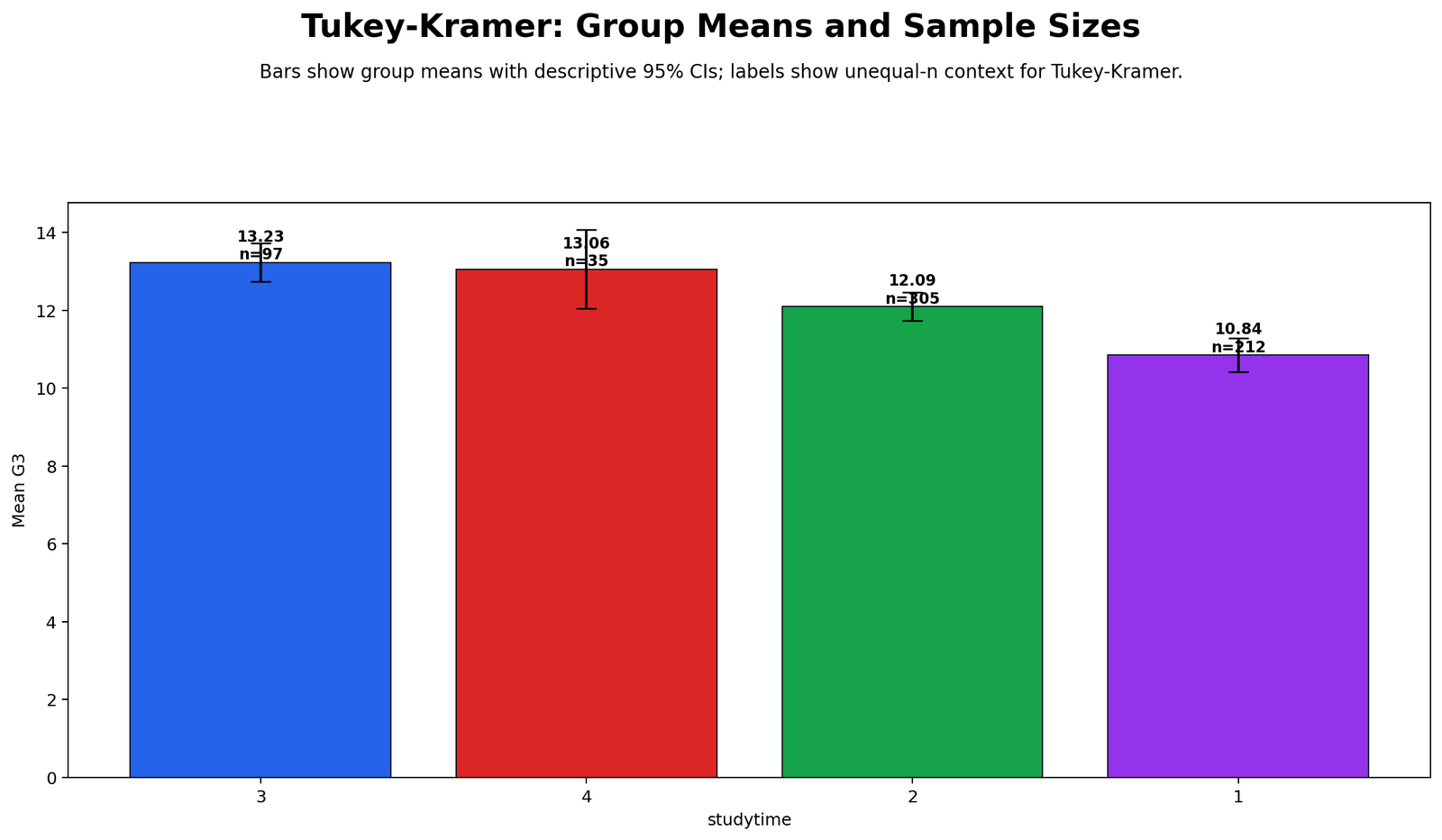
The first chart shows the four studytime group means. Group 1 has the lowest mean G3 score, 10.84, with n = 212. Group 2 is higher at 12.09, group 3 is highest at 13.23, and group 4 is close to group 3 at 13.06. The visual pattern already suggests that the lowest studytime group is separated from the higher studytime groups.
The sample-size labels are important because Tukey-Kramer does not treat every comparison as equally precise. Group 4 has only 35 observations, so its confidence interval is wider. This is why unequal-n adjustment matters: even if a mean looks high, a smaller group carries more uncertainty in pairwise testing.
Python Chart 2: Unequal-n Standard Errors
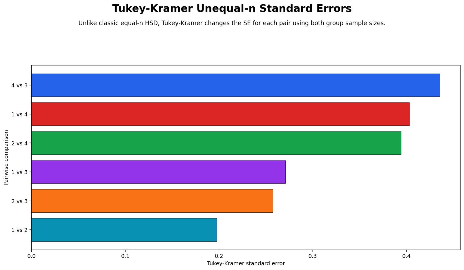
The unequal-n standard error chart shows why the Tukey-Kramer method is more appropriate than an equal-n shortcut here. The largest standard error belongs to 4 vs 3, because group 4 is the smallest group and group 3 is also smaller than group 2. The comparison 1 vs 2 has the smallest standard error because both groups are relatively large.
This chart explains why a mean difference cannot be judged by size alone. A pair with a moderate difference and a small standard error can become significant, while a pair with a similar difference and a large standard error may fail to reach significance. Tukey-Kramer builds this unequal precision into every comparison.
Python Chart 3: q Statistics vs Family-Wide Critical Value
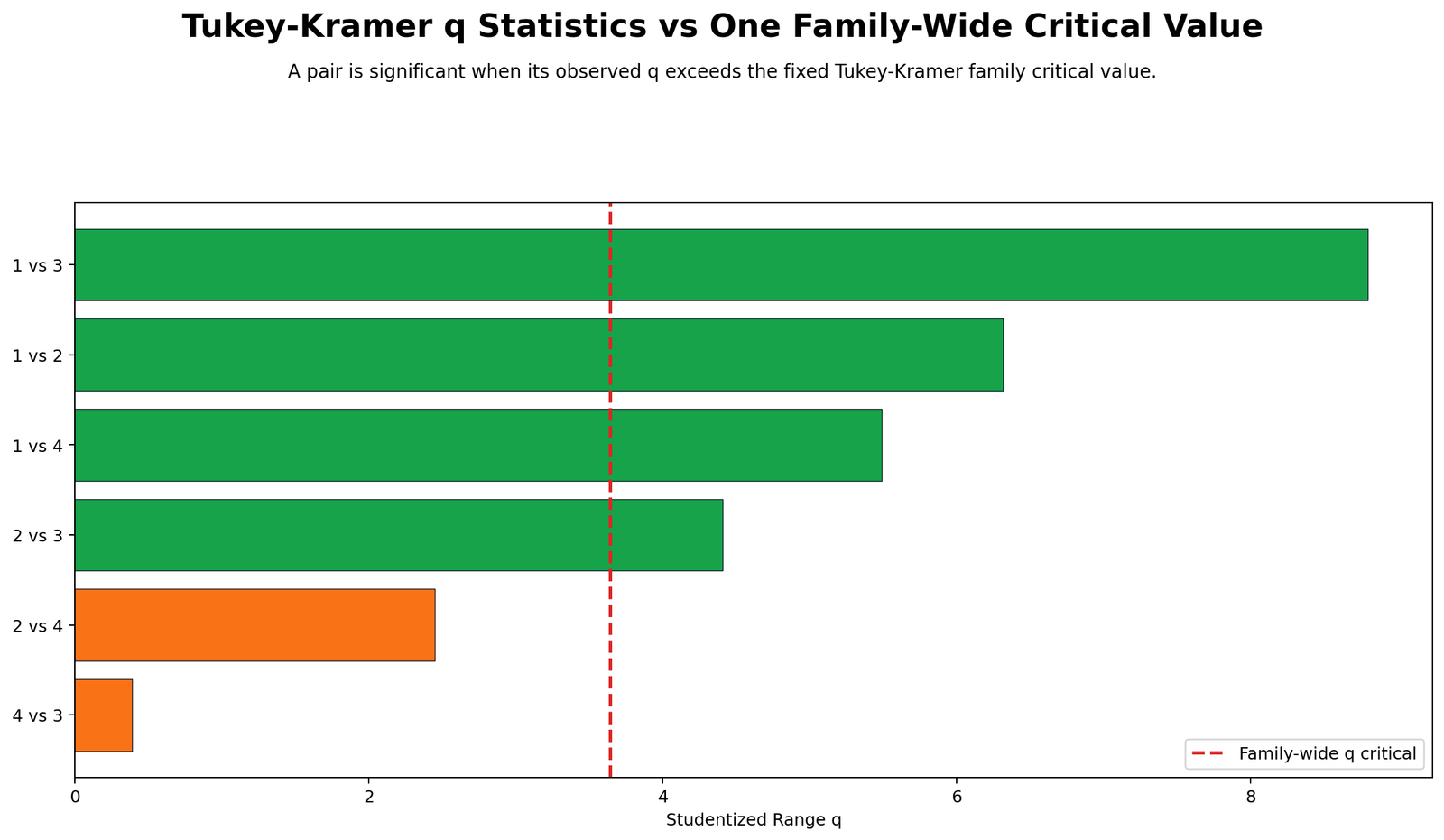
The red dashed line marks the family-wide q critical value of about 3.643. Any observed q statistic extending beyond this line is significant. The chart shows that 1 vs 3, 1 vs 2, 1 vs 4, and 2 vs 3 exceed the critical value, while 2 vs 4 and 4 vs 3 do not.
The strongest result is 1 vs 3, with q near 8.80. The weakest result is 4 vs 3, with q near 0.39, which is far below the critical value. This supports the conclusion that groups 3 and 4 are statistically similar in mean G3 score.
Python Chart 4: Adjusted p-value Ranking
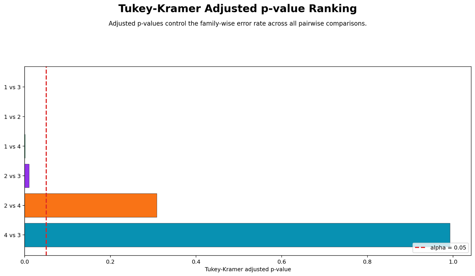
The adjusted p-value chart tells the same story from the p-value perspective. The vertical red line marks alpha = 0.05. Comparisons with bars to the left of this line are significant after family-wise adjustment. The comparisons involving group 1 against groups 2, 3 and 4 are significant, and the comparison 2 vs 3 is also significant.
The chart also makes the two non-significant comparisons clear. The adjusted p-value for 2 vs 4 is about 0.308, and the adjusted p-value for 4 vs 3 is about 0.993. These values are too large to reject the pairwise null hypothesis after controlling family-wise error.
Python Chart 5: Simultaneous Confidence Intervals
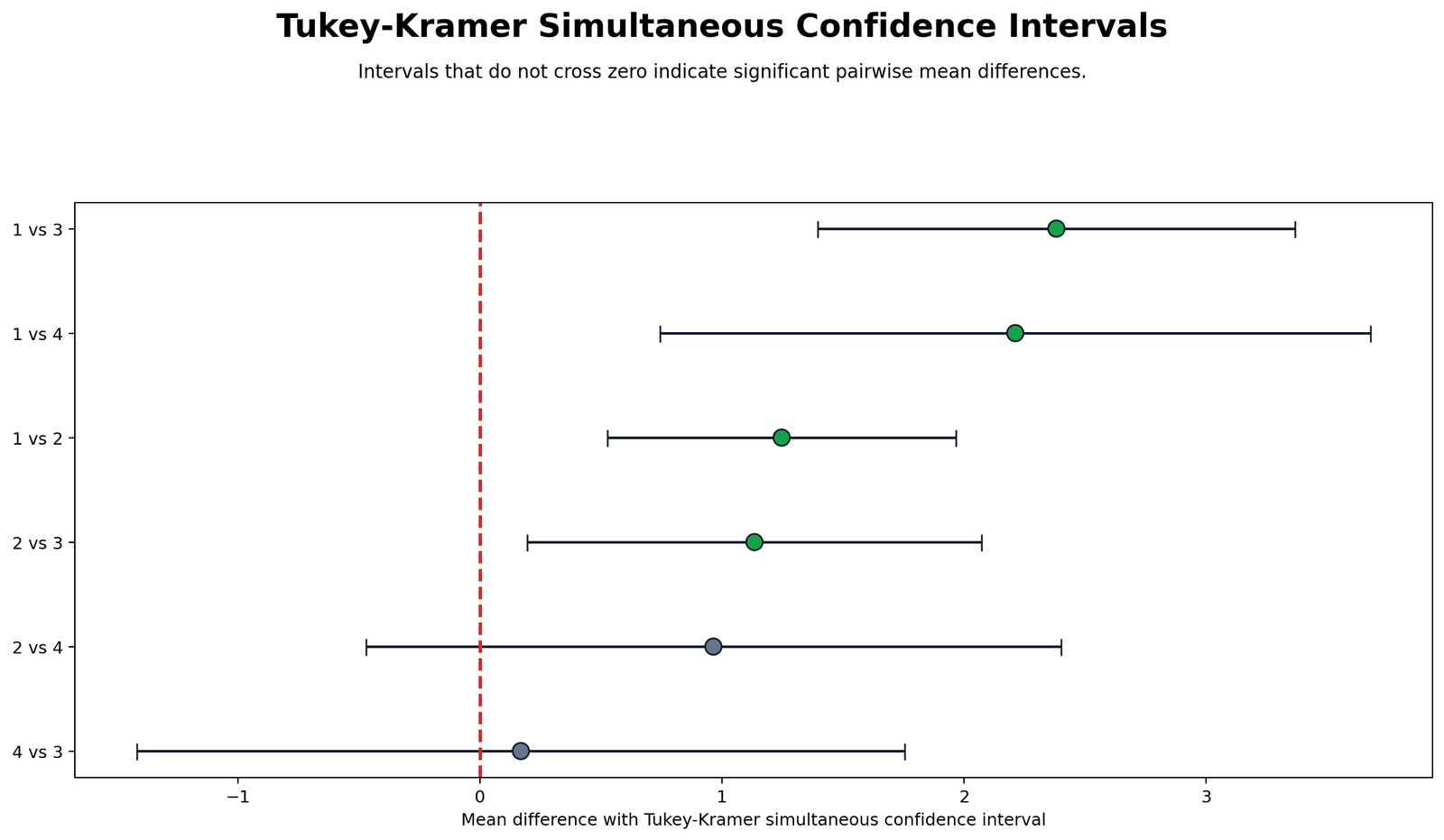
The simultaneous confidence interval chart shows pairwise mean differences with intervals adjusted for multiple comparisons. Intervals that do not cross zero indicate significant differences. The intervals for 1 vs 2, 1 vs 4, 1 vs 3, and 2 vs 3 stay entirely above zero, confirming those four significant results.
The intervals for 2 vs 4 and 4 vs 3 cross zero. That means the adjusted confidence interval allows a difference of zero, so those pairs are not statistically significant. This chart is often easier for readers than a p-value table because it shows both the direction and the uncertainty of each mean difference.
Python Chart 6: Pairwise Decision Matrix
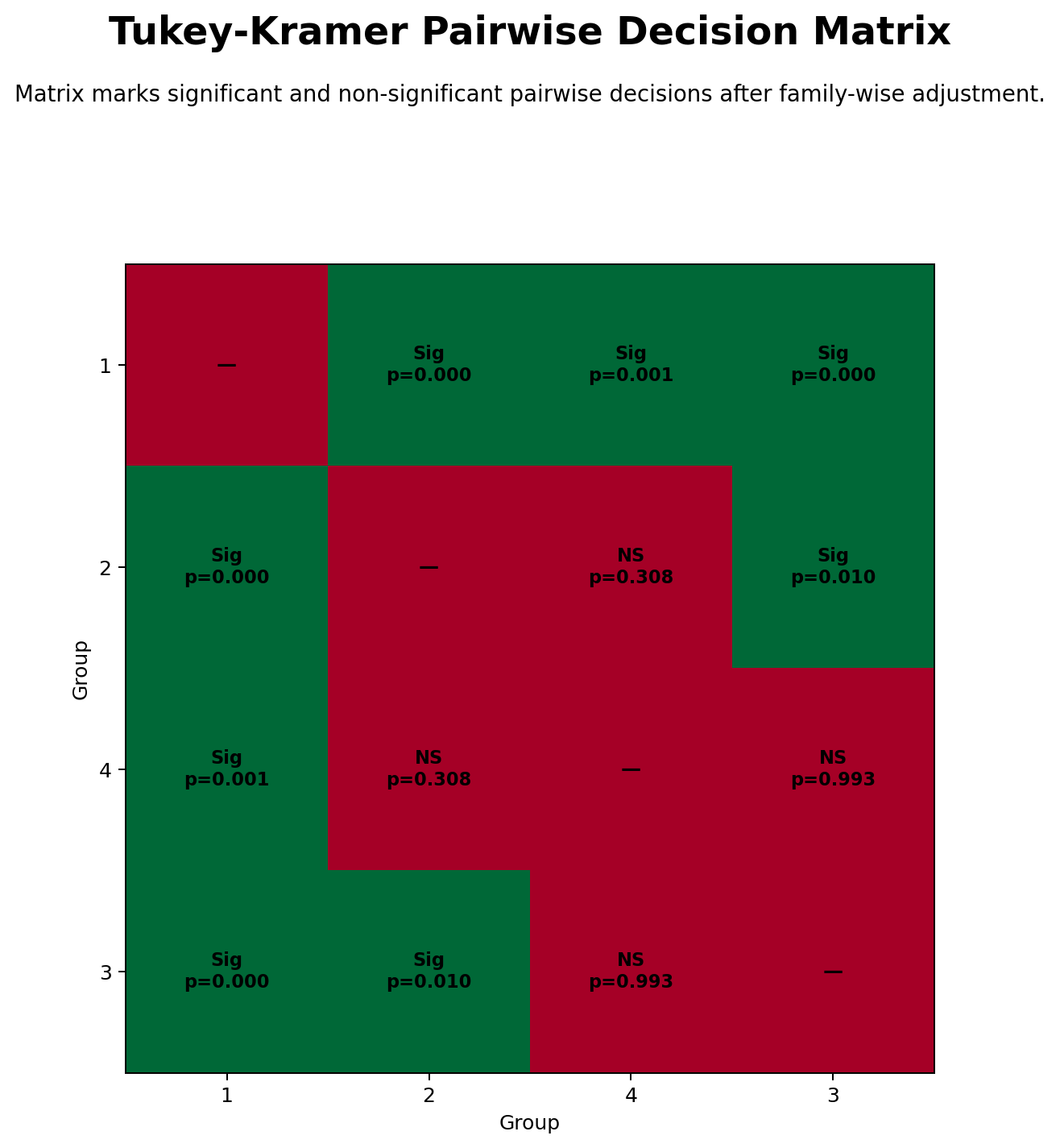
The decision matrix condenses the full post hoc result into a compact grid. The green cells mark significant pairwise differences and the red cells mark non-significant comparisons. Group 1 differs significantly from every other group, which confirms that the lowest studytime group is clearly separated from the others in mean G3 score.
The matrix also highlights the important upper-group pattern. Group 3 and group 4 are not significantly different, and group 2 and group 4 are also not significantly different after Tukey-Kramer adjustment. However, group 2 and group 3 are significantly different, showing that group 3 still stands above group 2 despite the family-wise correction.
Python Chart 7: Homogeneous Subset Letters
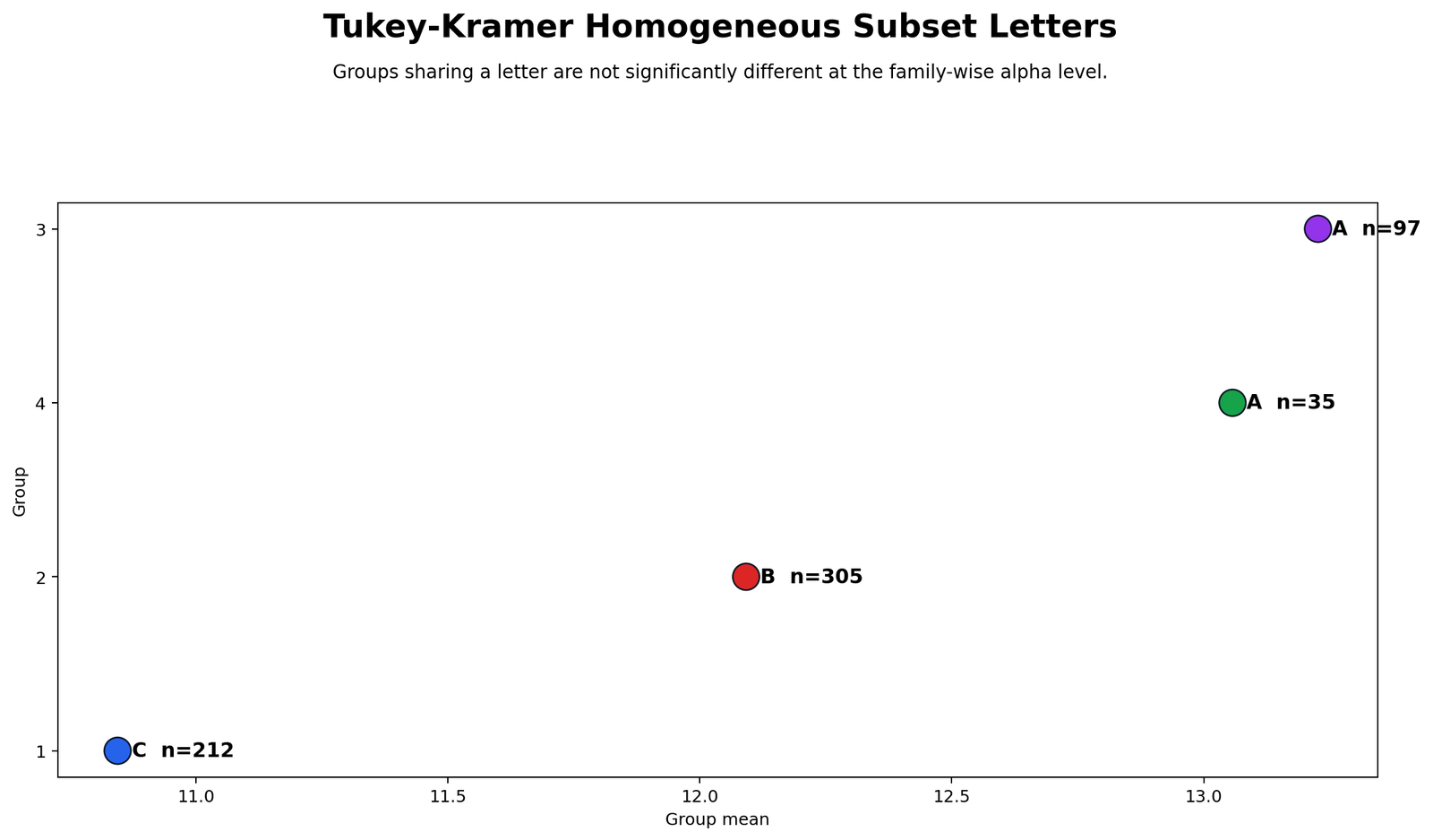
The homogeneous subset chart provides a report-friendly summary. Groups sharing a letter are not significantly different. Group 3 and group 4 both receive letter A, meaning they form the highest non-different subset. Group 2 receives letter B, and group 1 receives letter C.
This letter display is useful when there are many comparisons because it avoids making readers inspect every pair one by one. In this example, the final pattern is easy to explain: group 1 is the lowest subset, group 2 is the middle subset, and groups 3 and 4 are the highest subset.
Python Chart 8: Tukey-Kramer Method Report Card
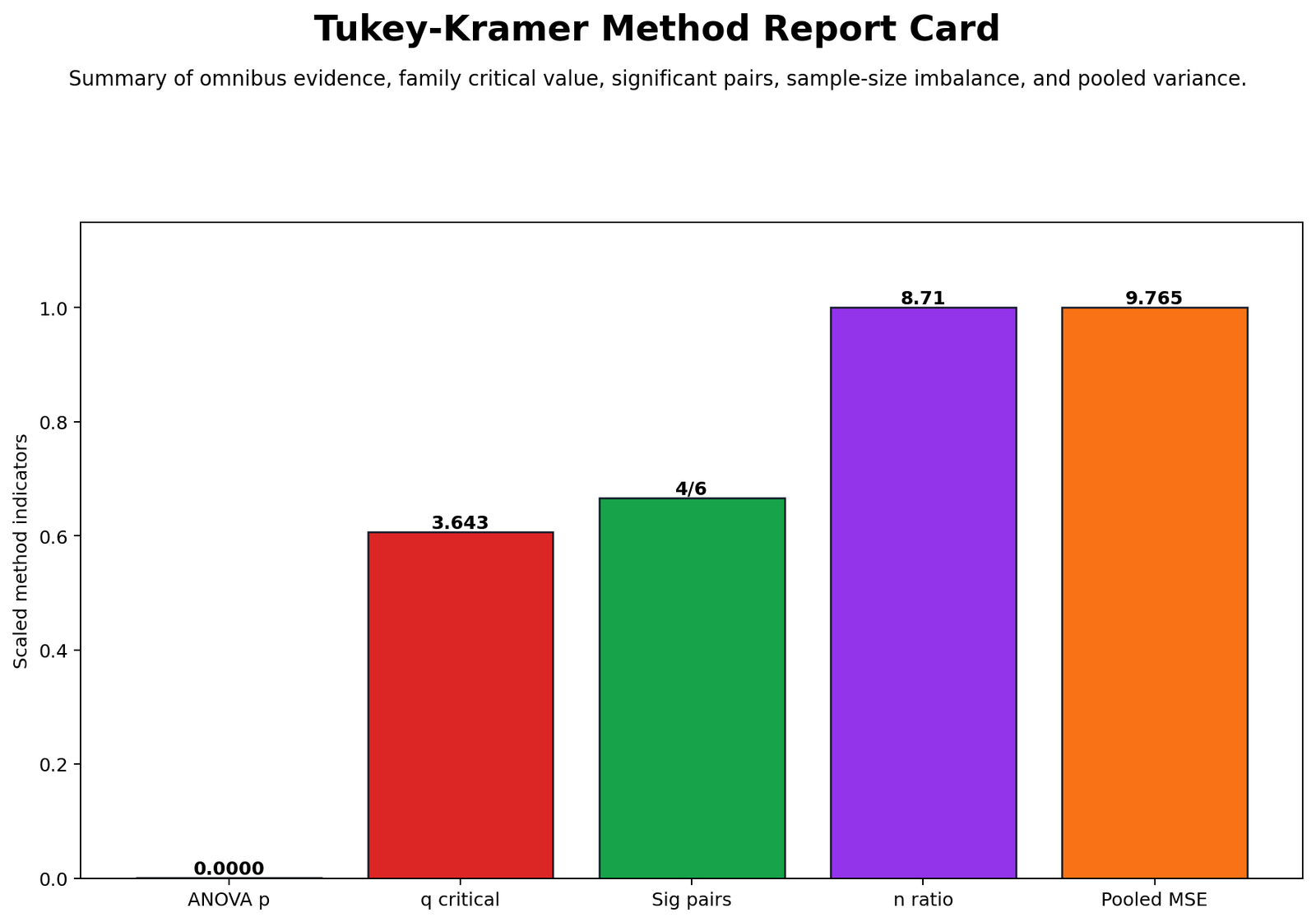
The method report card summarizes the key evidence needed for a complete Tukey-Kramer report. The ANOVA p-value is essentially zero at the displayed precision, the family-wide q critical value is 3.643, and 4 of 6 pairwise comparisons are significant. It also reports the sample-size imbalance and pooled MSE.
The n ratio of about 8.71 confirms why the Tukey-Kramer unequal-n version is appropriate. The pooled MSE of about 9.765 confirms the within-group error variance used to calculate every pairwise standard error. This chart is a good final dashboard for checking that the post hoc decision is supported by the ANOVA framework.
R Chart-by-Chart Validation
The R validation charts reproduce the same Tukey-Kramer logic with a separate workflow. Agreement between Python, R and SPSS strengthens confidence that the result is not a software artifact. The R charts below use the uploaded validation image set with the -1 filenames.
R Chart 1: Tukey-Kramer Group Means and Sample Sizes
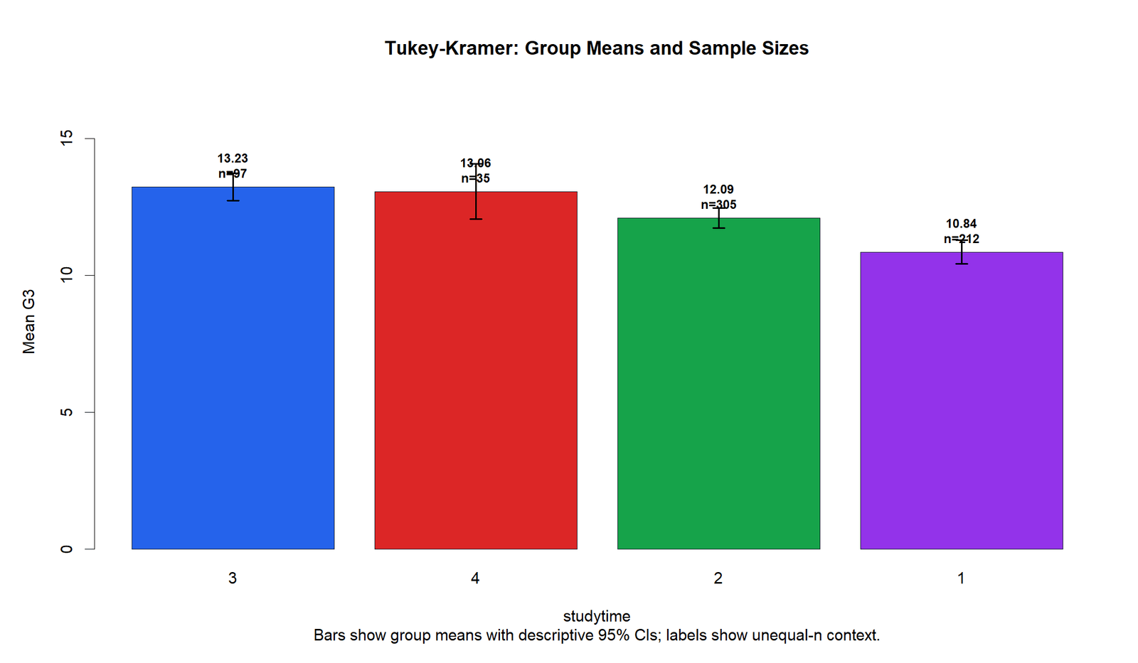
The R group mean chart validates the same descriptive pattern as Python. Studytime group 1 remains the lowest mean group, group 2 is higher, and groups 3 and 4 are the highest groups. The unequal sample sizes are again visible in the labels and the confidence interval widths.
This validation is important because post hoc interpretation begins with the descriptive pattern. The R chart confirms that the strongest practical separation is between the lowest studytime group and the higher studytime groups.
R Chart 2: Unequal-n Standard Errors
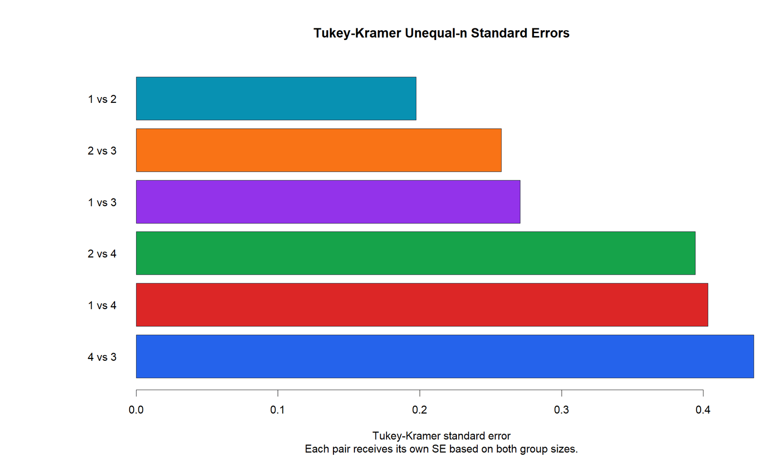
The R standard error chart confirms that the pairwise standard errors are not identical. Pairs involving the smallest group have larger uncertainty, while the largest groups produce more precise comparisons. This validates the unequal-n logic used in the test.
The chart also helps prevent a common reporting mistake. A Tukey-Kramer result should not be explained as if one identical standard error applied to every pair when the group sizes are unequal.
R Chart 3: q Statistics vs Family-Wide Critical Value
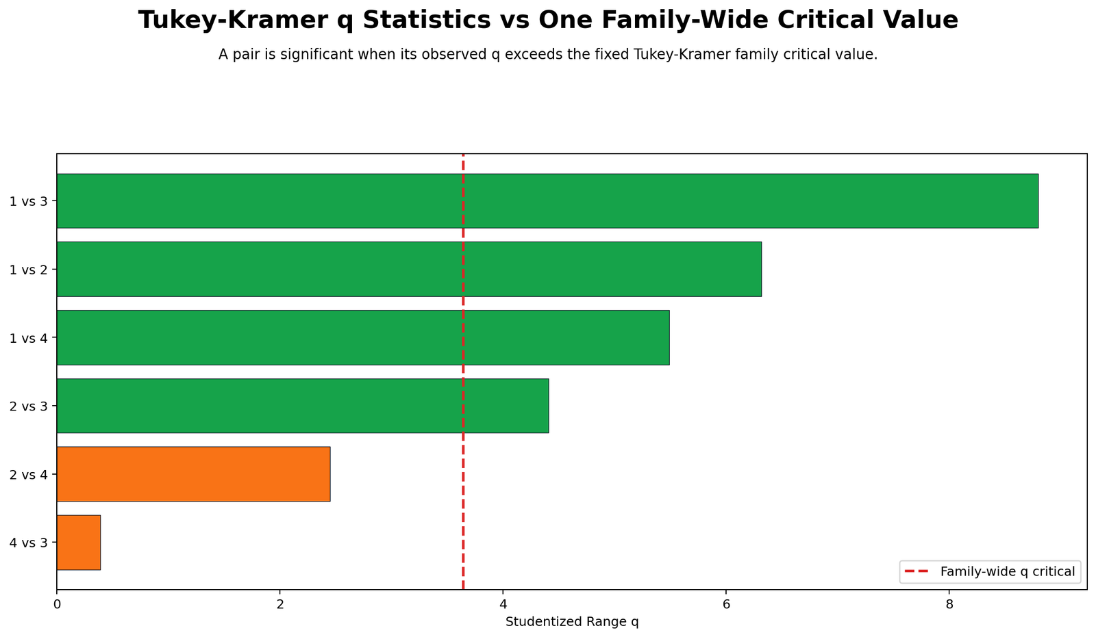
The R q statistic chart validates the same four significant comparisons. The bars for 1 vs 3, 1 vs 2, 1 vs 4 and 2 vs 3 exceed the family-wide q critical value. The bars for 2 vs 4 and 4 vs 3 stay below the threshold.
This chart is the direct visual decision rule for the Tukey-Kramer test. It confirms that the final pairwise decisions are supported by the studentized range distribution rather than by unadjusted t tests.
R Chart 4: Adjusted p-value Ranking
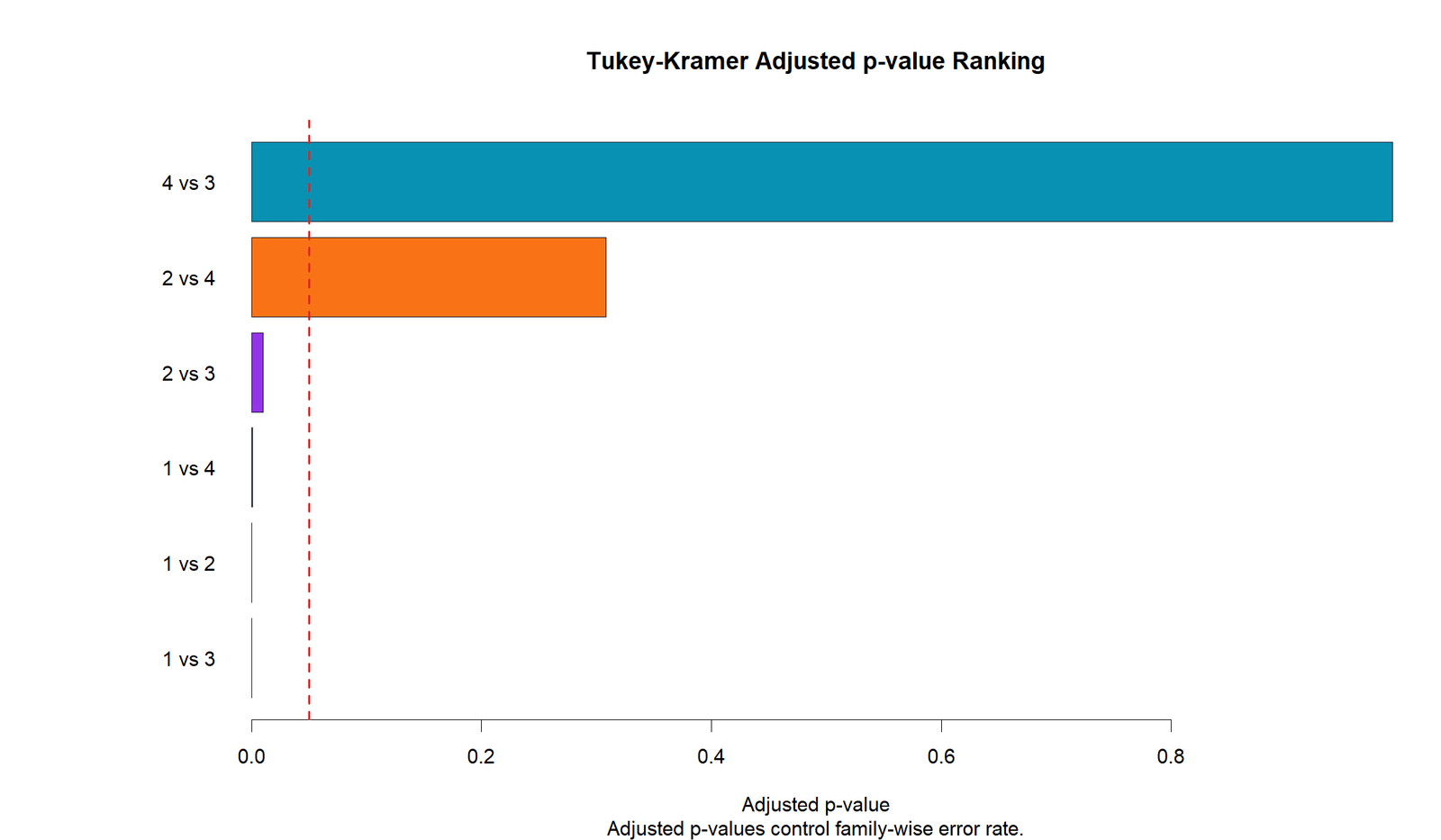
The R adjusted p-value ranking confirms that four comparisons are below alpha .05 after family-wise adjustment. The smallest adjusted p-value belongs to the largest mean separation, 1 vs 3. The comparison 4 vs 3 remains clearly non-significant.
This chart is useful for readers who prefer p-values over q statistics. It communicates that the significant decisions are not based on raw p-values but on Tukey-Kramer adjusted p-values.
R Chart 5: Simultaneous Confidence Intervals
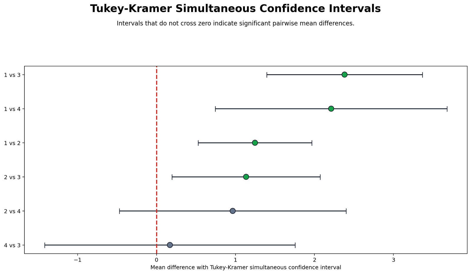
The R confidence interval chart confirms that significant pairs have intervals entirely above zero. The non-significant pairs cross zero, which matches the adjusted p-value and q statistic conclusions.
This validation supports a strong reporting style: report the adjusted p-values and also use simultaneous confidence intervals to explain the size and uncertainty of each pairwise difference.
R Chart 6: Pairwise Decision Matrix
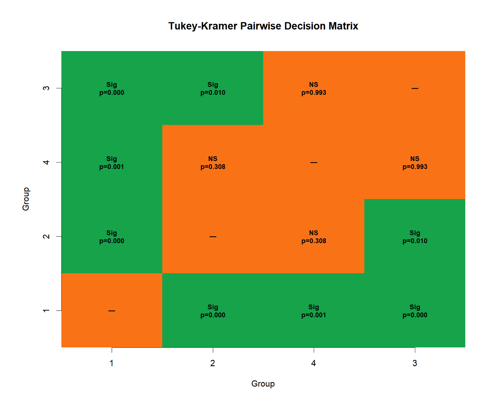
The R decision matrix validates the same final decision grid. Group 1 differs from every other studytime group, group 2 differs from group 3, and the two upper-level comparisons involving group 4 remain non-significant after adjustment.
The matrix is a helpful quality-control check because any mismatch between the q chart, p-value chart and confidence interval chart would be easy to detect. Here, all decision views agree.
R Chart 7: Homogeneous Subset Letters
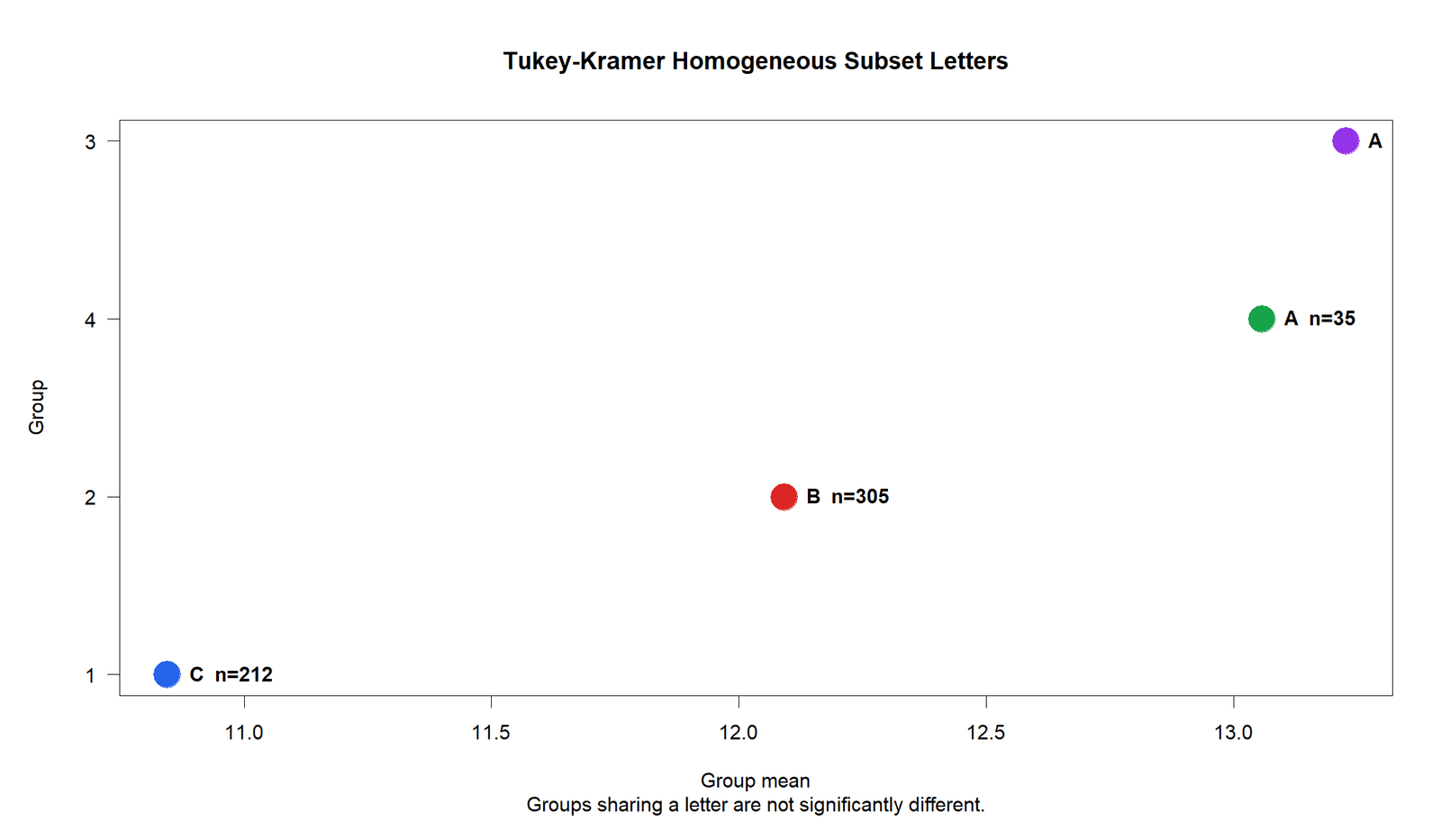
The R homogeneous subset chart confirms the final letter grouping: groups 3 and 4 share letter A, group 2 is letter B, and group 1 is letter C. Groups that do not share a letter should be interpreted as significantly different under the Tukey-Kramer family-wise rule.
This is often the most readable final summary for nontechnical readers. It turns six pairwise tests into a simple ordered group pattern.
R Chart 8: Tukey-Kramer Method Report Card
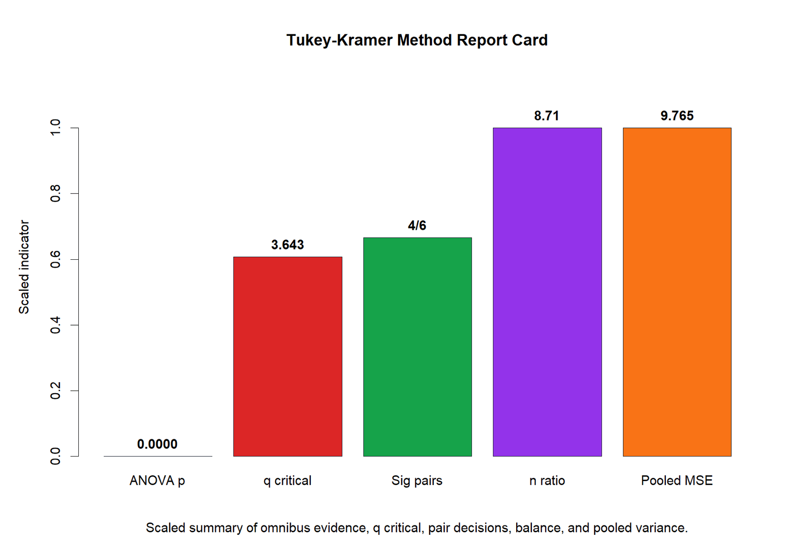
The R method report card validates the ANOVA p-value, q critical value, number of significant pairs, sample-size ratio and pooled MSE. These are the essential pieces needed for transparent reporting.
The agreement between Python and R supports the final conclusion: the Tukey-Kramer test detected four significant pairwise mean differences among studytime groups while controlling the family-wise error rate.
SPSS, R, Python and Excel Workflows for Tukey Kramer Test
The Tukey Kramer Test can be performed in SPSS, R, Python and Excel. The exact menu labels vary by software, but the logic is the same: run one-way ANOVA, confirm that a post hoc test is justified, calculate or request Tukey-Kramer pairwise comparisons, then interpret adjusted p-values, simultaneous confidence intervals and homogeneous subsets.
SPSS Workflow
| Step | SPSS Action | Purpose |
|---|---|---|
| Open dataset | File > Open > Data | Load the dataset containing G3 and studytime. |
| Run one-way ANOVA | Analyze > Compare Means > One-Way ANOVA | Set G3 as dependent variable and studytime as factor. |
| Request post hoc test | Post Hoc > Tukey | SPSS applies Tukey-style multiple comparisons and handles unequal sample sizes through the appropriate procedure. |
| Check homogeneity | Options > Homogeneity of variance test | Review Levene context before relying on equal-variance post hoc results. |
| Read output | Multiple Comparisons and Homogeneous Subsets | Interpret adjusted p-values, confidence intervals and subset letters. |
| Export report | File > Export PDF | Save the SPSS output for verification and reporting. |
R Workflow
| Step | R Action | Purpose |
|---|---|---|
| Read data | read.csv() | Load the dataset. |
| Fit ANOVA | aov(G3 ~ factor(studytime)) | Estimate the one-way ANOVA model. |
| Run Tukey comparison | TukeyHSD() | Generate adjusted pairwise comparisons. |
| Check assumptions | bartlett.test(), fligner.test(), or Levene-style tests | Check variance context before final interpretation. |
| Plot results | plot(TukeyHSD(model)) | Visualize simultaneous confidence intervals. |
Python Workflow
| Step | Python Action | Purpose |
|---|---|---|
| Read data | pandas.read_csv() | Load the dataset. |
| Fit ANOVA | statsmodels.formula.api.ols() | Estimate the ANOVA model. |
| Get ANOVA table | anova_lm() | Extract F statistic, p-value and pooled error term. |
| Run Tukey comparison | pairwise_tukeyhsd() or SciPy tukey_hsd() | Compute adjusted pairwise post hoc results. |
| Create custom Tukey-Kramer table | Use pooled MSE, unequal-n SE and studentized range critical value | Show transparent q statistics, adjusted p-values and simultaneous CIs. |
Excel Workflow
Excel can calculate Tukey-Kramer manually if the ANOVA summary table is available. You need the group means, group sample sizes, pooled MSE, error degrees of freedom, number of groups and a studentized range critical value. The most difficult part is obtaining the correct studentized range critical value and adjusted p-values; many users rely on add-ins, statistical tables or external calculation tools for that step.
| Excel Input | Where It Comes From | Use in Tukey-Kramer |
|---|---|---|
| Group means | AVERAGEIF or PivotTable | Used in the numerator of the q statistic. |
| Group sample sizes | COUNTIF or PivotTable | Used in the unequal-n standard error. |
| Pooled MSE | ANOVA within-group mean square | Used as pooled error variance. |
| q critical | Studentized range table or software | Used to judge statistical significance. |
| Simultaneous CI | Mean difference ± q critical × SE | Used to interpret direction and uncertainty. |
Code Blocks for Tukey Kramer Test
Python Code
import pandas as pd
import statsmodels.api as sm
from statsmodels.formula.api import ols
from statsmodels.stats.multicomp import pairwise_tukeyhsd

# Load data
df = pd.read_csv("dataset.csv")

# Keep valid observations
df = df[["G3", "studytime"]].dropna()
df["studytime"] = df["studytime"].astype("category")

# One-way ANOVA
model = ols("G3 ~ C(studytime)", data=df).fit()
anova_table = sm.stats.anova_lm(model, typ=2)
print(anova_table)

# Tukey-style post hoc comparison
tukey = pairwise_tukeyhsd(
    endog=df["G3"],
    groups=df["studytime"],
    alpha=0.05
)
print(tukey)

# Group summary
summary = df.groupby("studytime")["G3"].agg(["count", "mean", "std"])
print(summary)
R Code
# Load data
df <- read.csv("dataset.csv")

# Keep valid observations
df <- na.omit(df[, c("G3", "studytime")])
df$studytime <- factor(df$studytime)

# One-way ANOVA
model <- aov(G3 ~ studytime, data = df)
summary(model)

# Tukey post hoc comparison
tukey_result <- TukeyHSD(model, "studytime", conf.level = 0.95)
print(tukey_result)

# Plot simultaneous confidence intervals
plot(tukey_result)
SPSS Syntax
ONEWAY G3 BY studytime
  /STATISTICS DESCRIPTIVES HOMOGENEITY
  /POSTHOC = TUKEY ALPHA(0.05)
  /MISSING ANALYSIS.

OUTPUT EXPORT
  /CONTENTS EXPORT=ALL
  /PDF DOCUMENTFILE='Tukey-Kramer-Test-SPSS-Output.pdf'.
Excel Formula Pattern
Mean difference:
=ABS(mean_i - mean_j)

Tukey-Kramer standard error:
=SQRT((MSE/2) * ((1/n_i) + (1/n_j)))

q statistic:
=ABS(mean_i - mean_j) / SQRT((MSE/2) * ((1/n_i) + (1/n_j)))

Simultaneous confidence interval lower:
=Mean_Difference - q_critical * Standard_Error

Simultaneous confidence interval upper:
=Mean_Difference + q_critical * Standard_Error

Decision:
=IF(q_statistic > q_critical, "Significant", "Not significant")
APA Reporting Wording for Tukey Kramer Test
APA-style reporting should first state the ANOVA result and then summarize the post hoc comparisons. The report should include the test name, the reason for using it, the adjusted comparison results and the interpretation of significant pairs. Avoid reporting only “Tukey was significant” because the test is pairwise; each comparison has its own decision.
APA-style example: A one-way ANOVA showed that mean G3 scores differed significantly across studytime groups, F(3, 645) = 15.88, p < .001, η² = .069. Tukey-Kramer post hoc comparisons were used because group sample sizes were unequal. The results showed that group 1 scored significantly lower than group 2, group 4 and group 3. Group 2 also scored significantly lower than group 3. The comparisons between group 2 and group 4 and between group 4 and group 3 were not statistically significant after family-wise adjustment.
For a more detailed report, include adjusted p-values and simultaneous confidence intervals. For example, the difference between studytime group 1 and group 3 was significant, mean difference = 2.38, adjusted p < .001, simultaneous CI [1.40, 3.37]. The comparison between group 4 and group 3 was not significant, mean difference = 0.17, adjusted p = .993, simultaneous CI [-1.42, 1.76].
Common Mistakes in Tukey Kramer Test
| Mistake | Why It Is a Problem | Better Practice |
|---|---|---|
| Running Tukey-Kramer without checking ANOVA context | Post hoc tests should be connected to the omnibus model and assumptions. | Report ANOVA, MSE, df error and variance context. |
| Using unadjusted p-values for all pairs | Multiple comparisons inflate Type I error. | Use adjusted Tukey-Kramer p-values or simultaneous CIs. |
| Ignoring unequal sample sizes | Unequal n changes each pairwise standard error. | Use the Tukey-Kramer unequal-n standard error formula. |
| Calling every different-looking mean significant | Visual mean differences may be explained by sampling uncertainty. | Use q statistic, adjusted p-value and simultaneous CI decision rules. |
| Using Tukey-Kramer under serious variance heterogeneity | The method relies on pooled ANOVA MSE. | Consider Games-Howell or Tamhane’s T2 if heterogeneity is serious. |
| Reporting only homogeneous letters | Letters are useful but do not show effect sizes or intervals. | Report letters with mean differences, adjusted p-values and confidence intervals. |
Downloads and Resources
The following report files and visual outputs support the Tukey Kramer Test example. Use them to verify the Python output, R validation and SPSS reporting.
Python Report PDF
ANOVA summary, Tukey-Kramer comparisons, q statistics, adjusted p-values and charts.
R Report PDF
R validation output for group summaries, post hoc comparisons and visual checks.
SPSS Output PDF
SPSS one-way ANOVA and post hoc output for reporting verification.
External References
FAQs About Tukey Kramer Test
What is the Tukey Kramer Test?
The Tukey Kramer Test is a post hoc multiple comparison method used after ANOVA to compare all pairs of group means while controlling the family-wise error rate. It is especially useful when sample sizes are unequal.
When should I use the Tukey Kramer Test?
Use it after a significant one-way ANOVA when you want all pairwise group comparisons and the equal-variance assumption is acceptable. It is particularly suitable when the group sample sizes are not equal.
What does a Tukey Kramer Test tell you?
It tells you which specific pairs of group means differ significantly after adjusting for multiple comparisons. ANOVA tells you that at least one mean differs; Tukey-Kramer tells you where the differences are.
Is Tukey Kramer the same as Tukey HSD?
They are closely related. Tukey-Kramer is commonly described as the unequal-sample-size version of Tukey HSD. With equal sample sizes, the methods are very similar.
What is q in the Tukey Kramer Test?
The q statistic is the studentized range statistic. It divides the absolute pairwise mean difference by the Tukey-Kramer standard error and compares the result with a family-wide q critical value.
How do I interpret adjusted p-values in Tukey Kramer Test?
An adjusted p-value below alpha, usually .05, means the pairwise mean difference is significant after controlling the family-wise error rate across all pairwise comparisons.
Can I do Tukey Kramer Test in Excel?
Yes, but it is easiest when you already have the ANOVA MSE, group means, group sample sizes, error degrees of freedom and studentized range critical value. Excel can calculate the q statistic and confidence intervals manually, but adjusted p-values usually require an add-in or external calculation.
What should I use if variances are unequal?
If variance heterogeneity is serious, consider alternatives such as Games-Howell or Tamhane’s T2. Tukey-Kramer uses pooled ANOVA error variance, so it is best when the equal-variance context is acceptable.

