
Unequal Variance Post Hoc Test, Welch ANOVA and Multiple Comparisons
Tamhane’s T2 Test: Formula, SPSS, Python, R and Excel Post Hoc Guide
Tamhane’s T2 test is an unequal-variance post hoc procedure used after one-way ANOVA or Welch ANOVA when researchers need pairwise group comparisons but do not want to assume equal variances. This complete guide explains the Tamhane T2 test with verified group descriptives, Welch standard errors, adjusted p values, confidence intervals, SPSS workflow, Python charts, R validation, Excel method, APA wording, common mistakes and downloadable report resources.
Quick Answer: Tamhane’s T2 Test Result
The worked example compares G3 final grade across four weekly study time groups: <2 hours, 2 to 5 hours, 5 to 10 hours, and >10 hours. The sample includes 649 valid cases. Group means increased from 10.84 for students studying less than 2 hours to 13.23 for students studying 5 to 10 hours, while the >10 hours group had a mean of 13.06.
The Welch ANOVA context was statistically significant, F(3, 139.10) = 18.18, p < .001, supporting follow-up pairwise comparisons. The Tamhane-style unequal-variance pairwise table found 4 significant comparisons out of 6 at alpha = .05. The significant differences were <2 hours vs 2 to 5 hours, <2 hours vs 5 to 10 hours, <2 hours vs >10 hours, and 2 to 5 hours vs 5 to 10 hours. The comparisons 2 to 5 hours vs >10 hours and 5 to 10 hours vs >10 hours were not significant after adjustment.
Final interpretation: The Tamhane’s T2 test shows that students in the lowest studytime group had significantly lower final grades than each higher studytime group. The strongest adjusted difference was between <2 hours and 5 to 10 hours, with a mean difference of about 2.38 grade points and an adjusted p value near 1.02 × 10⁻¹⁰. The two highest studytime groups were statistically similar after adjustment.
Important SPSS syntax note: In SPSS One-Way ANOVA syntax, Tamhane’s T2 is commonly requested as /POSTHOC = T2, not as the full word TAMHANE. The article below uses the corrected SPSS workflow so the pairwise table can be generated properly.
Table of Contents
- What Is Tamhane’s T2 Test?
- When Should You Use Tamhane T2?
- Tamhane’s T2 Formula and Decision Logic
- Null and Alternative Hypotheses
- Dataset and Variables Used
- Verified Results and Pairwise Comparison Table
- SPSS Output Interpretation
- Python Chart-by-Chart Interpretation
- R Chart-by-Chart Validation
- SPSS, R, Python and Excel Workflows
- Code Blocks for Tamhane’s T2
- APA Reporting Wording
- Common Mistakes
- Downloads and Resources
- Related Guides
- FAQs
What Is Tamhane’s T2 Test?
Tamhane’s T2 test is a post hoc multiple comparison method designed for pairwise group comparisons when equal variances cannot be safely assumed. In simple terms, it compares every pair of group means while using unequal-variance logic instead of forcing all groups to share the same pooled error variance.
A standard one-way ANOVA may tell you that at least one group mean differs from another, but it does not tell you exactly which groups are different. A post hoc test answers the pairwise question. If the groups have similar variances and balanced sample sizes, tests such as Tukey HSD are often used. If variances or sample sizes are unequal, Tamhane T2 becomes more appropriate because each pair receives its own standard error and degrees of freedom.
The phrase Tamhane’s T2 variances not assumed is common in SPSS output and search queries because the method belongs to the family of post hoc tests used when the equal-variance assumption is questionable. It is especially useful for educational, psychological, medical, business, and social science data where groups often have unequal sample sizes and unequal spreads.
Simple definition: Tamhane’s T2 is a conservative unequal-variance post hoc test. It compares group means pair by pair, uses a Welch-style standard error, adjusts for multiple comparisons, and helps identify which specific groups differ after a significant omnibus test.
Before using this guide, it is helpful to understand one-way ANOVA, ANOVA assumptions, Levene’s test, and Brown-Forsythe variance testing. These guides explain why post hoc selection depends on the equality-of-variance assumption.
When Should You Use Tamhane T2?
Use Tamhane T2 when you have one categorical independent variable with three or more groups, one continuous dependent variable, and you need pairwise post hoc comparisons without assuming equal group variances. It is often selected after a significant one-way ANOVA or a significant Welch ANOVA when the research question requires group-by-group interpretation.
| Situation | Use Tamhane’s T2? | Reason |
|---|---|---|
| Three or more independent groups | Yes | Tamhane’s T2 is a post hoc test for pairwise comparisons among multiple independent groups. |
| Dependent variable is continuous | Yes | The method compares group means on a numeric outcome such as final grade, score, income, blood pressure, or performance. |
| Equal variances are not assumed | Yes | The method uses unequal-variance standard errors rather than a pooled ANOVA error term. |
| Sample sizes are unequal | Often yes | Unequal n makes pooled-variance post hoc tests more fragile, especially when group spreads differ. |
| Only two groups are being compared | No | Use an independent samples t test or Welch’s t test instead. |
| Groups are repeated measures | No | Tamhane’s T2 assumes independent groups, not repeated measurements from the same participants. |
In this example, the factor is studytime, the dependent variable is G3 final grade, there are four groups, and the sample sizes are unequal: 212, 305, 97 and 35. Even though the median-centered Levene/Brown-Forsythe context was not significant, the unequal sample sizes make Tamhane’s T2 a useful conservative teaching example for comparing studytime groups.
Tamhane’s T2 Formula and Decision Logic
The first step is the mean difference between two groups. For any two groups i and j, the pairwise mean difference is:
The unequal-variance standard error for the pair is calculated from each group’s own variance and sample size:
The test statistic compares the absolute mean difference with the unequal-variance standard error:
The degrees of freedom are estimated with Welch-Satterthwaite logic, so every pair can have a different degrees-of-freedom value. Then the p value or confidence interval is adjusted for the number of pairwise comparisons. In the Python and R workflow used here, the Tamhane-style table uses Welch standard errors, Welch degrees of freedom and Sidak-adjusted p values.
| Component | Meaning | Why It Matters |
|---|---|---|
| X̄i, X̄j | Two group means | The test asks whether the two group averages are far enough apart to be statistically meaningful. |
| si2, sj2 | Two group variances | Each group keeps its own variance instead of forcing a pooled variance assumption. |
| ni, nj | Two group sample sizes | Unequal sample sizes affect the standard error and the precision of each comparison. |
| Welch df | Pair-specific degrees of freedom | Pairs with smaller or more variable groups receive different degrees-of-freedom values. |
| Adjusted p value | Multiple-comparison corrected p | Protects against inflated Type I error when many pairwise comparisons are tested. |
Reporting rule: Do not report only the omnibus ANOVA result. A complete Tamhane’s T2 report should include group means, sample sizes, the omnibus Welch or ANOVA context, adjusted pairwise p values, confidence intervals and a plain-language conclusion.
Null and Alternative Hypotheses for Tamhane’s T2
The omnibus ANOVA or Welch ANOVA tests whether all group means are equal. Tamhane’s T2 then tests pairwise null hypotheses for every group pair. For each pair, the null hypothesis says that the two group means are equal, and the alternative hypothesis says that they differ.
| Comparison Level | Null Hypothesis | Alternative Hypothesis | Decision Rule |
|---|---|---|---|
| Omnibus Welch ANOVA | All studytime group means are equal. | At least one studytime group mean is different. | Use the Welch ANOVA p value to decide whether follow-up comparisons are needed. |
| Pairwise Tamhane T2 | Group i mean = Group j mean. | Group i mean ≠ Group j mean. | Use adjusted p value and adjusted confidence interval for each pair. |
| Practical interpretation | The two groups perform similarly. | The two groups differ in average G3 score. | Report the direction, difference size and statistical significance. |
Decision for this example: The Welch ANOVA was significant, and Tamhane’s T2 found four significant pairwise differences. The lowest studytime group had significantly lower G3 scores than the other three groups. The 5 to 10 hours and >10 hours groups were not significantly different from each other.
Dataset and Variables Used
The worked example uses a student performance dataset. The dependent variable is G3 final grade, and the grouping variable is studytime. The studytime factor has four ordered categories: <2 hours, 2 to 5 hours, 5 to 10 hours, and >10 hours. The goal is to determine which studytime groups have different average final grades after adjusting for multiple pairwise comparisons.
| Variable | Role | Values Used | Why It Matters |
|---|---|---|---|
| G3 | Dependent variable | Final grade score | This is the continuous outcome compared across studytime groups. |
| studytime | Grouping factor | 1, 2, 3, 4 | This creates the four independent groups used in the post hoc test. |
| Group 1 | Studytime category | <2 hours | This is the lowest studytime group and the main lower-mean group in the results. |
| Group 2 | Studytime category | 2 to 5 hours | This group is higher than group 1 but lower than group 3. |
| Group 3 | Studytime category | 5 to 10 hours | This group has the highest mean G3 score in the example. |
| Group 4 | Studytime category | >10 hours | This group has a high mean but a small sample size, so unequal-variance post hoc logic is useful. |
Before interpreting post hoc tests, it is good practice to inspect descriptive statistics, box plots, histograms, standard deviations, variances, and the five-number summary. These summaries explain why some pairwise tests are precise while others have wider confidence intervals.
Verified Results and Pairwise Comparison Table
The group descriptive statistics show a clear upward pattern from the lowest studytime group to the moderate and high studytime groups. The variance ratio was about 1.68, which is not extremely large, and the median-centered Levene/Brown-Forsythe context was not significant. However, the group sample sizes were unequal, especially for the >10 hours group with only 35 cases. Tamhane’s T2 remains useful because it does not require the equal-variance assumption.
Group Summary for G3 by Studytime
| Studytime Group | n | Mean | Std. Deviation | Std. Error | Variance | 95% CI for Mean | Interpretation |
|---|---|---|---|---|---|---|---|
| <2 hours | 212 | 10.84 | 3.219 | .221 | 10.360 | 10.41 to 11.28 | Lowest mean final grade group. |
| 2 to 5 hours | 305 | 12.09 | 3.243 | .186 | 10.518 | 11.73 to 12.46 | Higher than the lowest studytime group. |
| 5 to 10 hours | 97 | 13.23 | 2.502 | .254 | 6.261 | 12.73 to 13.72 | Highest mean final grade group. |
| >10 hours | 35 | 13.06 | 3.038 | .514 | 9.232 | 12.05 to 14.06 | High mean but wider uncertainty because the group is small. |
Omnibus Context Before Tamhane’s T2
| Test | Statistic | df | p value | Interpretation |
|---|---|---|---|---|
| Classic one-way ANOVA | F = 15.876 | 3, 645 | < .001 | There is an overall difference among studytime group means. |
| Welch ANOVA | F = 18.183 | 3, 139.101 | < .001 | The robust unequal-variance context also supports follow-up comparisons. |
| Median-centered Levene/Brown-Forsythe | 1.026 | 3, 645 | .380 | No strong evidence of unequal variances, but Tamhane remains valid and conservative. |
Tamhane’s T2 Pairwise Comparison Results
| Comparison | Mean Difference | Welch SE | Welch df | Adjusted p | Adjusted 95% CI | Decision |
|---|---|---|---|---|---|---|
| <2 hours vs 2 to 5 hours | 1.247 | .289 | 456.20 | .000115 | .485 to 2.010 | Significant |
| <2 hours vs >10 hours | 2.213 | .559 | 47.50 | .00151 | .678 to 3.748 | Significant |
| <2 hours vs 5 to 10 hours | 2.382 | .337 | 235.09 | 1.02e-10 | 1.489 to 3.276 | Significant |
| 2 to 5 hours vs >10 hours | .965 | .546 | 43.39 | .410 | -.540 to 2.471 | Not significant |
| 2 to 5 hours vs 5 to 10 hours | 1.135 | .315 | 207.30 | .00233 | .299 to 1.971 | Significant |
| >10 hours vs 5 to 10 hours | .170 | .573 | 51.58 | .9998 | -1.398 to 1.737 | Not significant |
The pairwise table shows that the lowest studytime group is consistently lower than the other groups. The 2 to 5 hours group is also significantly lower than the 5 to 10 hours group. However, the >10 hours group is not significantly higher than the 2 to 5 hours group and is almost identical to the 5 to 10 hours group. This means the result supports a clear improvement from very low studytime to moderate studytime, but it does not prove that studying more than 10 hours produces a higher mean than studying 5 to 10 hours.
SPSS Output Interpretation for Tamhane’s T2
The SPSS output verifies the group descriptives, variance context, classic ANOVA, Welch ANOVA and visual group mean pattern. The SPSS descriptive table shows that all 649 cases were included, with no excluded cases. The mean final grade increased from 10.84 in the <2 hours group to 13.23 in the 5 to 10 hours group.
The SPSS homogeneity section shows Levene results based on mean, median, adjusted median and trimmed mean. The median-based version was p = .380, so the output does not show strong variance inequality. Still, Tamhane’s T2 is appropriate as a conservative unequal-variance post hoc explanation, especially because the group sample sizes are unbalanced.
The SPSS ANOVA context shows a significant classic ANOVA, F(3, 645) = 15.876, p < .001, and a significant Welch robust test, F(3, 139.101) = 18.183, p < .001. These results justify pairwise follow-up testing. The correct SPSS syntax for Tamhane’s T2 in the One-Way ANOVA command should use /POSTHOC = T2 ALPHA(.05).
SPSS correction note: If SPSS reports that the word TAMHANE is not recognized on the POSTHOC subcommand, use T2. The corrected syntax is shown in the SPSS code section below.
Python Chart-by-Chart Interpretation
The Python charts provide a clean visual explanation of the Tamhane T2 test. They show the group mean profile, variance and sample size context, Welch standard error pattern, adjusted p values, adjusted confidence intervals, decision matrix, Welch degrees of freedom and method report card.
Python Chart 1: Unequal-Variance Group Profile
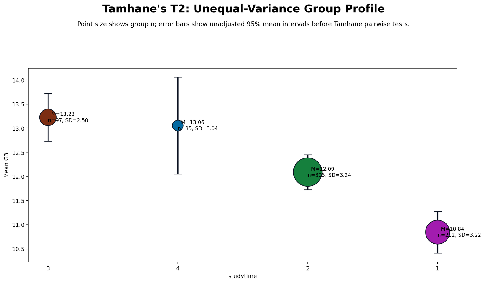
This chart shows the central result visually. The <2 hours group has the lowest mean G3 score, while the 5 to 10 hours group has the highest mean. The >10 hours group is also high, but it is based on a much smaller sample, so the visual interpretation should be combined with the adjusted pairwise comparisons.
The chart supports the final conclusion that very low studytime is associated with lower final grades. However, the curve does not continue upward after 5 to 10 hours. The highest and longest studytime groups are close to each other, which explains why the Tamhane comparison between 5 to 10 hours and >10 hours is not significant.
Python Chart 2: Variance vs Sample Size
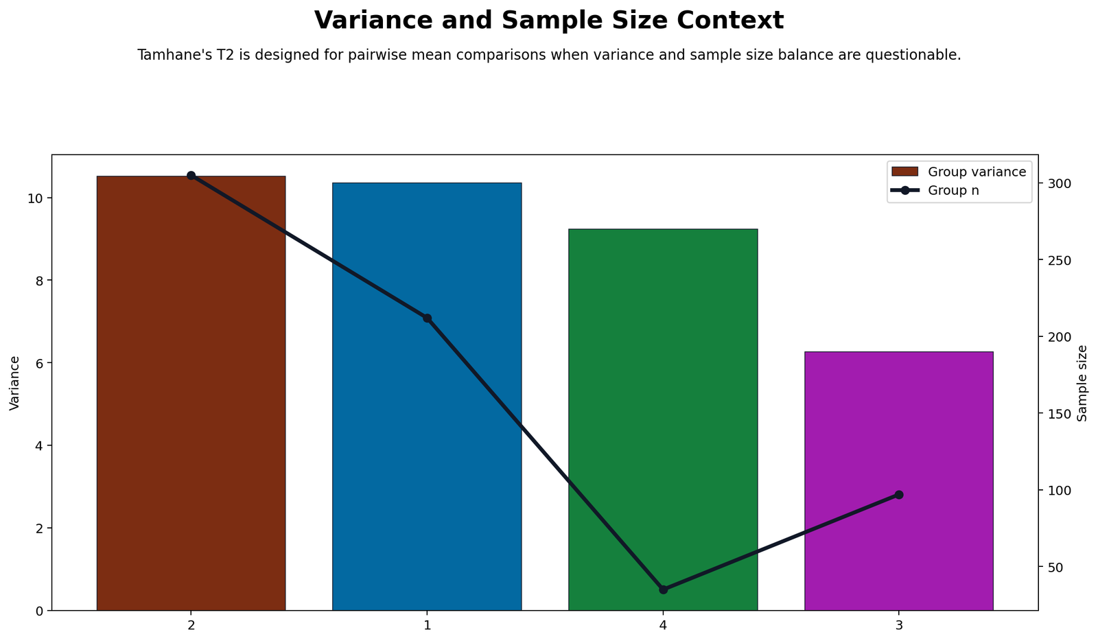
This chart explains why Tamhane’s T2 is relevant. The group variances are not identical, and the sample sizes are clearly unequal. The largest group has 305 cases, while the >10 hours group has only 35 cases. A pooled-variance post hoc test would treat group variation more uniformly than this design deserves.
The chart also shows that the 5 to 10 hours group has the smallest variance, while the first two groups have larger variances. Tamhane’s T2 handles this kind of structure by calculating pair-specific uncertainty instead of relying on one pooled ANOVA error term.
Python Chart 3: Welch Standard Error Map
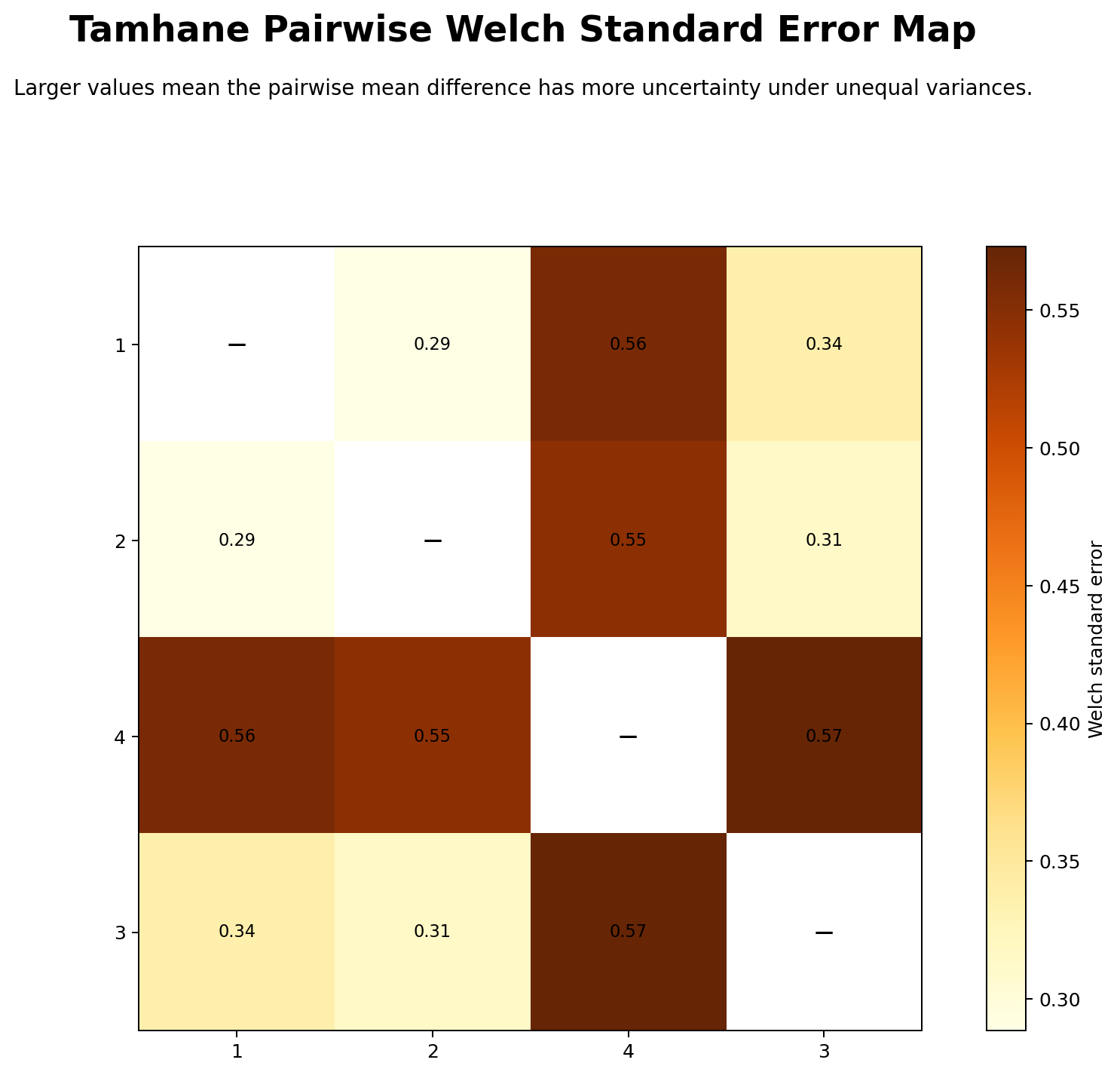
The Welch standard error map shows that not every pairwise comparison has the same precision. Comparisons involving the small >10 hours group have larger standard errors because that group has only 35 observations. Larger standard errors make it harder for a mean difference to become significant after adjustment.
This is why the 2 to 5 hours versus >10 hours difference is not significant even though the mean difference is close to 0.97 points. The uncertainty around that pair is too wide after adjustment, so the adjusted confidence interval includes zero.
Python Chart 4: Pairwise Adjusted p Values
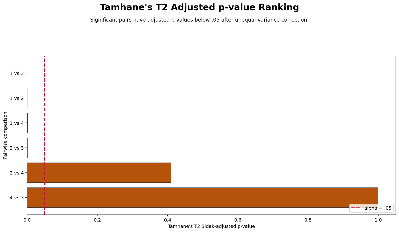
This chart translates the pairwise table into a simple decision view. Four comparisons have adjusted p values below .05, and two comparisons do not. The strongest evidence appears for <2 hours versus 5 to 10 hours, where the adjusted p value is extremely small.
The adjusted p value chart is especially helpful for reporting because it prevents over-reading unadjusted pairwise tests. The result should be interpreted from the adjusted p values, not from ordinary uncorrected t tests.
Python Chart 5: Mean Differences with Adjusted Confidence Intervals
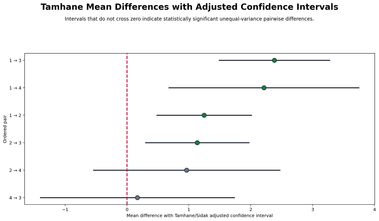
This confidence interval chart gives the best interpretation of direction and uncertainty. A significant comparison has an adjusted confidence interval that does not cross zero. The differences involving the <2 hours group clearly stay above zero, showing that higher studytime groups had higher mean G3 scores.
The non-significant comparisons have intervals that cross zero. This is why the >10 hours group should not be described as significantly better than the 2 to 5 hours group, and why the 5 to 10 hours group should not be described as significantly different from the >10 hours group.
Python Chart 6: Tamhane Decision Matrix
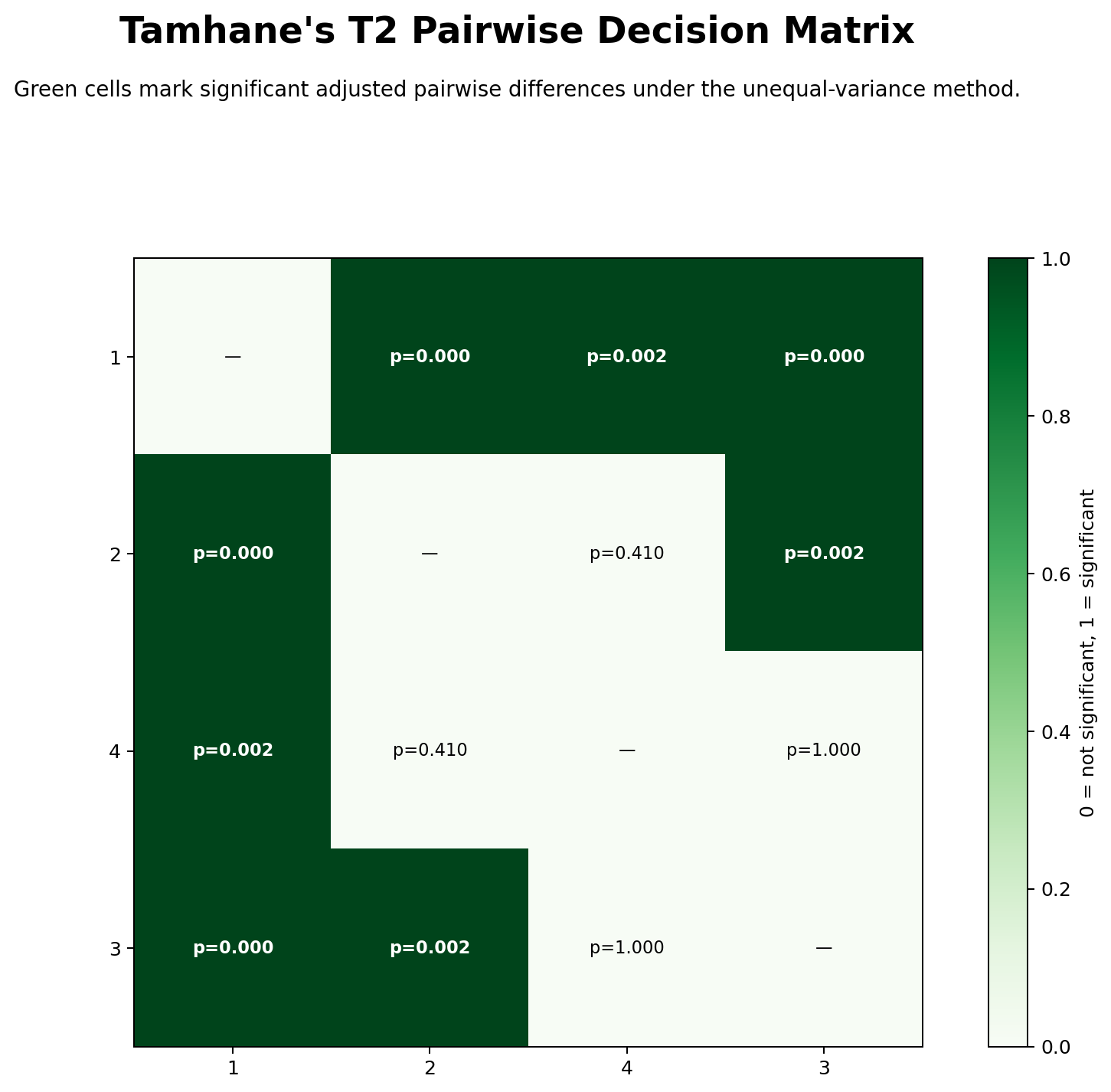
The decision matrix is a compact summary of the entire post hoc test. It shows significant differences between the lowest studytime group and all other groups, plus a significant difference between 2 to 5 hours and 5 to 10 hours. It also shows no significant difference for the two pairs involving the highest studytime group where confidence intervals include zero.
This matrix is useful when writing the result section because it avoids long repetitive wording. The final interpretation can focus on the pattern: group 1 is lower than groups 2, 3 and 4; group 2 is lower than group 3; groups 3 and 4 are statistically similar.
Python Chart 7: Welch Degrees of Freedom Heatmap
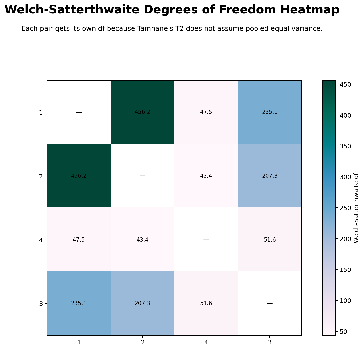
The degrees-of-freedom heatmap shows why Tamhane’s T2 is not the same as a pooled-variance post hoc test. Pairs with large sample sizes have high degrees of freedom, while comparisons involving the small >10 hours group have much lower degrees of freedom.
This pair-specific adjustment is one of the main reasons Tamhane’s T2 is preferred when variances or sample sizes are not equal. It gives each pair a more realistic uncertainty estimate.
Python Chart 8: Method Report Card
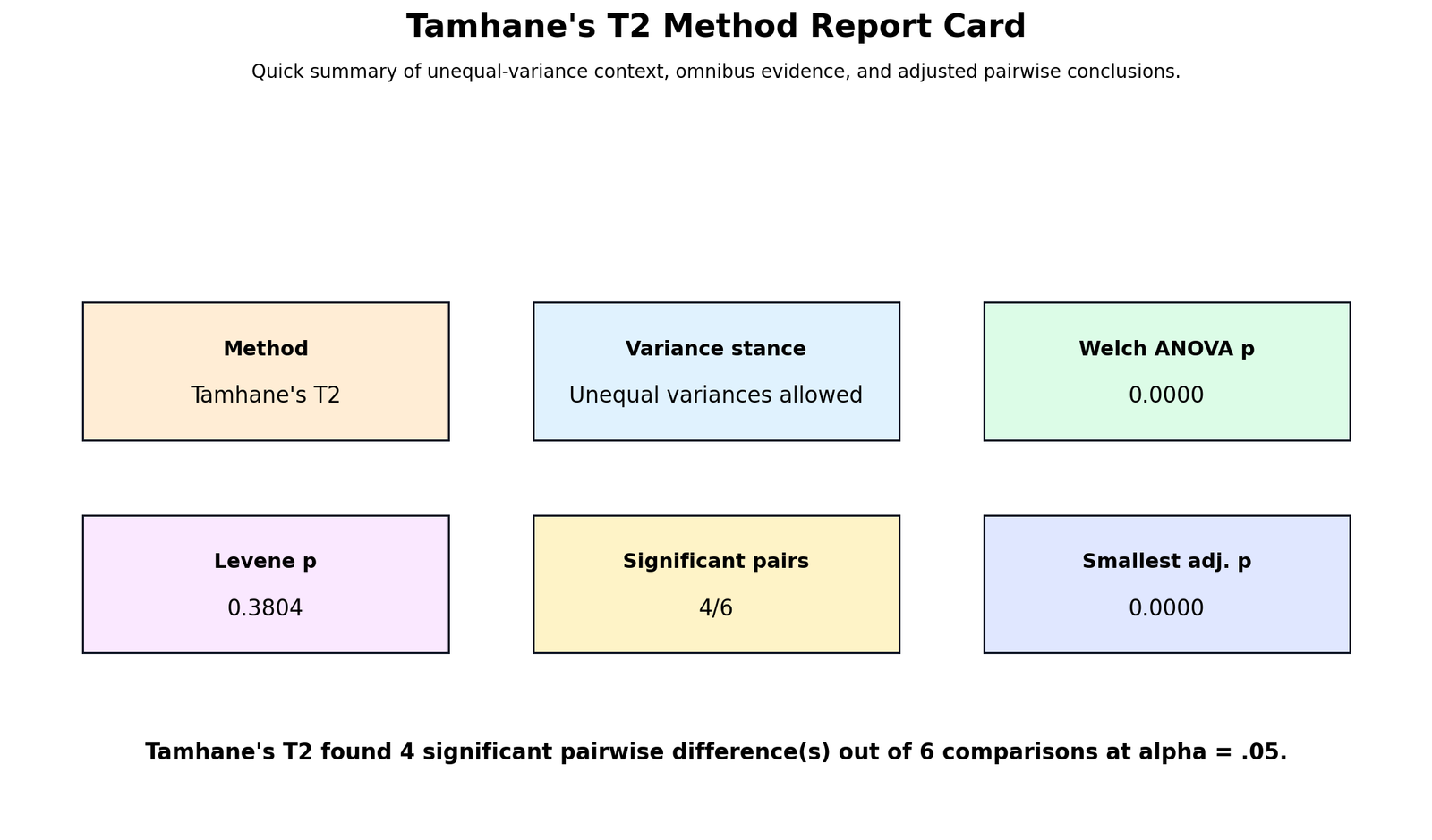
The method report card collects the most important result details in one place. It confirms that the dependent variable is G3, the factor is studytime, the method is Tamhane’s T2, there are four groups, the sample size is 649, and four out of six pairwise comparisons are significant.
This chart is useful for final checking before publication. It ensures that the written report matches the statistical output: Welch ANOVA is significant, the lowest studytime group is the main source of differences, and the final post hoc conclusion should be based on adjusted pairwise decisions.
R Chart-by-Chart Validation
The R charts validate the Python results using a separate workflow. The same visual pattern appears: studytime group means increase from the lowest group to the moderate groups, uncertainty differs by pair, and the adjusted pairwise decisions match the Python summary.
R Chart 1: Unequal-Variance Group Profile
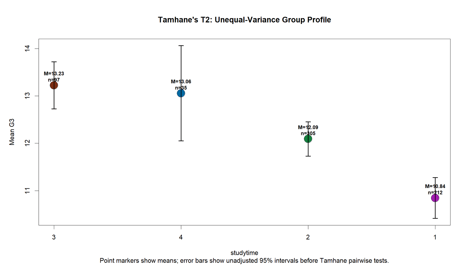
The R group profile confirms the Python pattern. Students in the <2 hours group have the lowest mean G3 score, while students in the 5 to 10 hours and >10 hours groups have higher means.
The chart validates that the main result is not caused by one software package. Both Python and R show the same direction: the lowest studytime group is the clear lower-performing group.
R Chart 2: Variance vs Sample Size
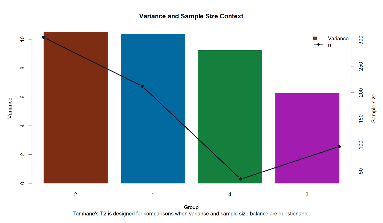
The R variance and sample size chart confirms the same design issue as Python: the groups are not equally sized. The first two groups are much larger than the >10 hours group, so pairwise uncertainty is not identical across comparisons.
This supports the use of an unequal-variance post hoc method. Even when Levene’s test is not significant, unbalanced group sizes can make a robust post hoc explanation more defensible for teaching and reporting.
R Chart 3: Welch Standard Error Map
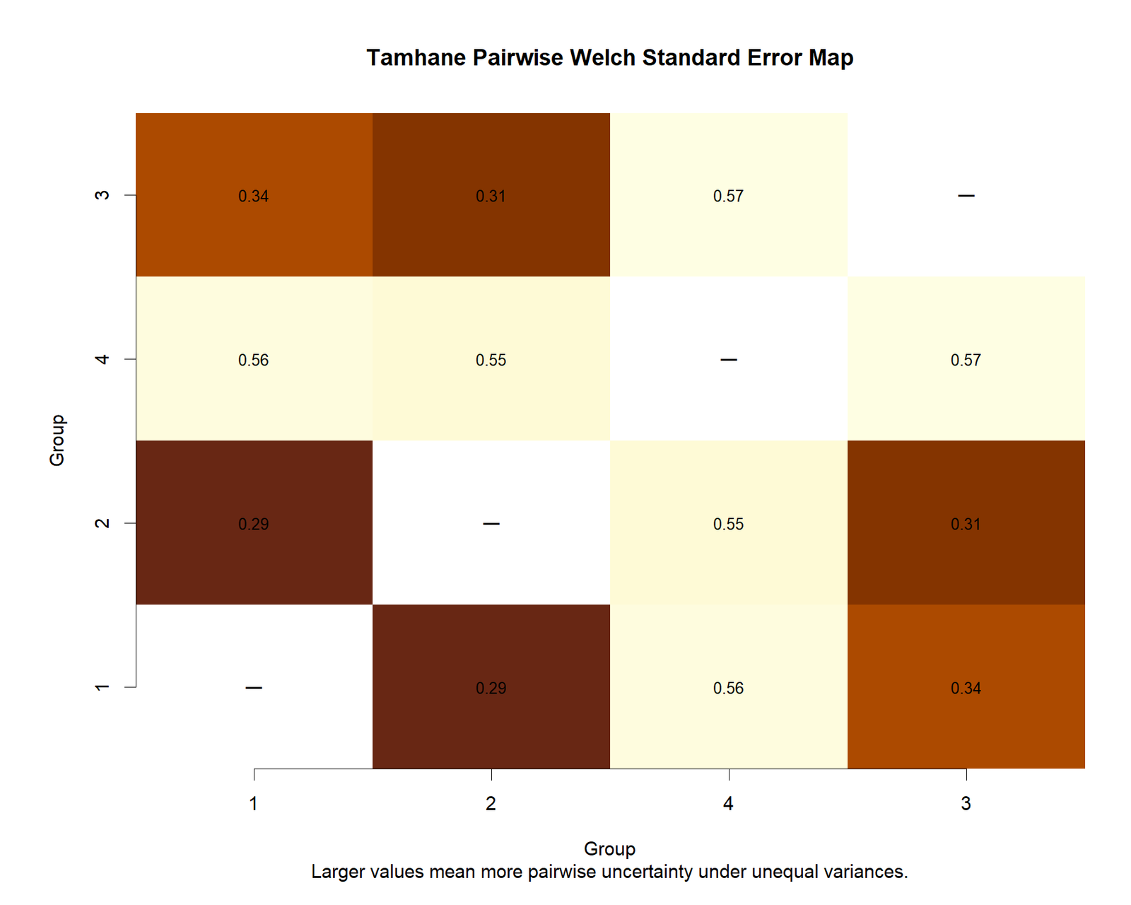
The R standard error map confirms that comparisons involving the smallest group have higher uncertainty. This explains why some mean differences are not significant even when the group means are numerically separated.
For example, the >10 hours group has a high mean, but its small sample size increases pairwise standard errors. The post hoc decision must therefore use adjusted p values and confidence intervals, not only raw mean differences.
R Chart 4: Pairwise Adjusted p Values
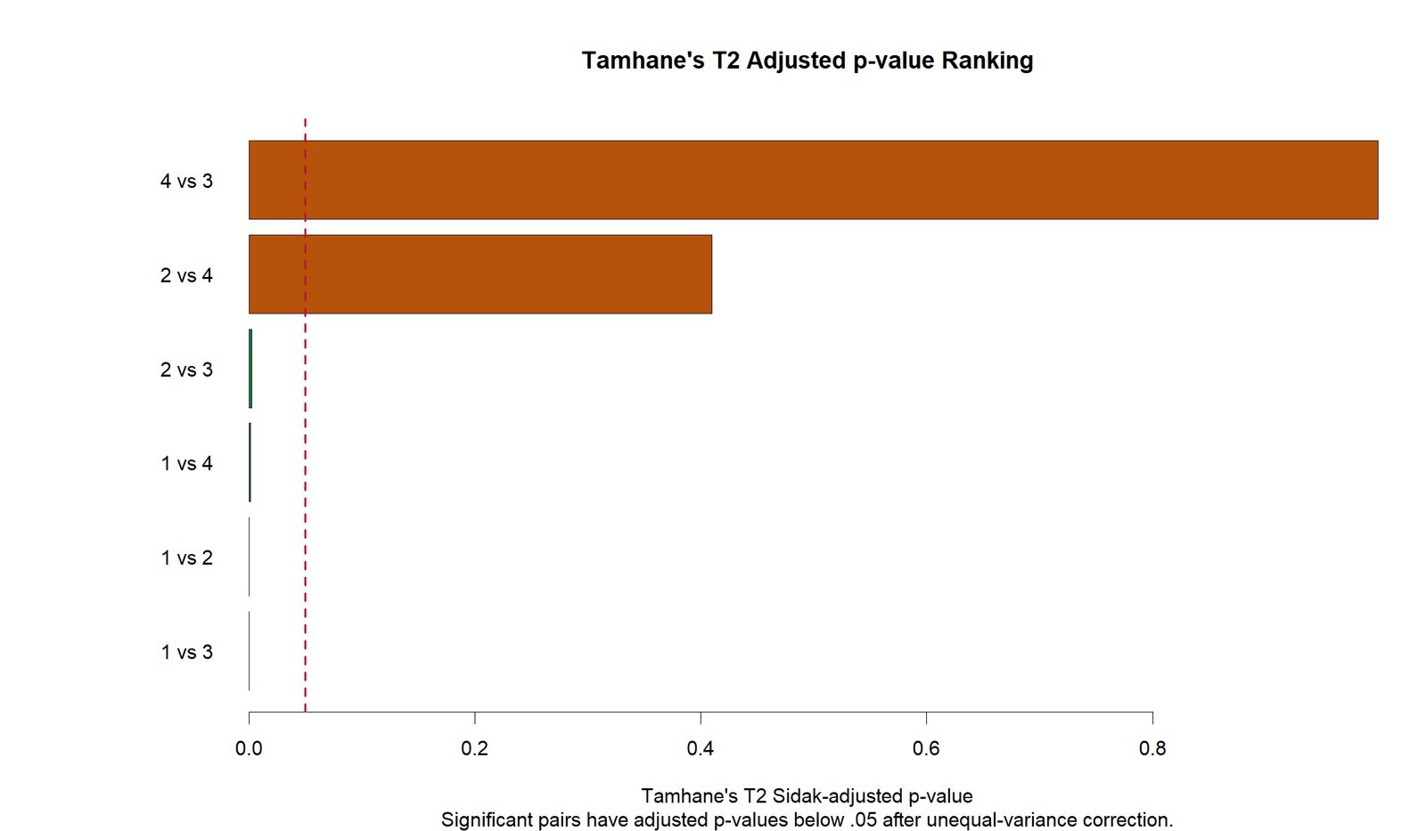
The R adjusted p value chart confirms the four significant and two non-significant pairwise decisions. The smallest adjusted p value belongs to the comparison between <2 hours and 5 to 10 hours.
This agreement strengthens the final reporting conclusion. The main statistically supported story is a difference between very low studytime and moderate-to-higher studytime, not a simple claim that every higher studytime category differs from every other category.
R Chart 5: Mean Differences with Adjusted Confidence Intervals
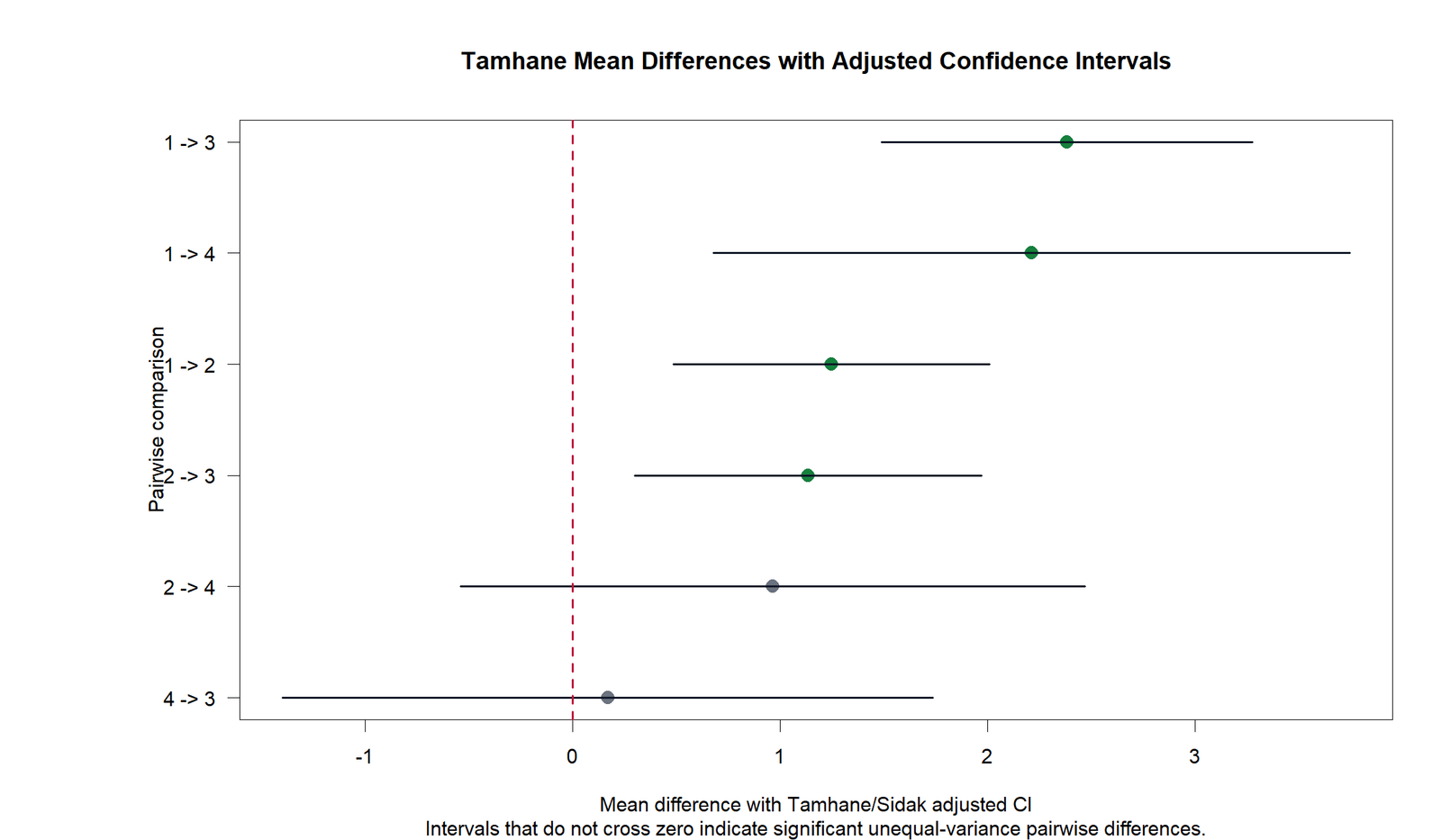
The R confidence interval chart confirms the same interpretation as the Python chart. Significant intervals do not cross zero, while non-significant intervals include zero.
This chart is the best visual for explaining practical direction. It shows exactly which groups have higher average G3 scores and which pairwise differences remain uncertain after adjustment.
R Chart 6: Decision Matrix
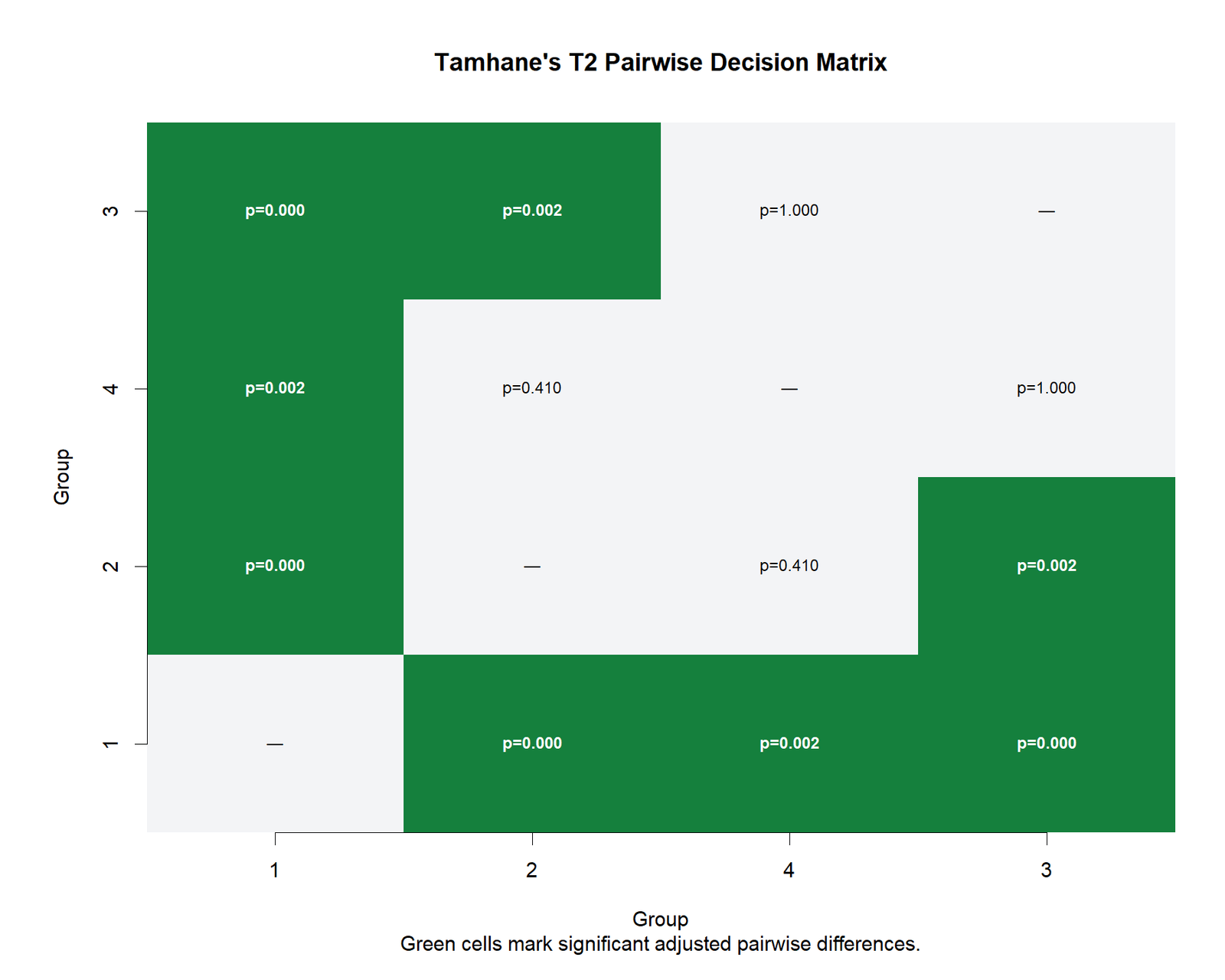
The R decision matrix confirms the final pairwise pattern. The lowest group differs from the other groups, the 2 to 5 hours group differs from the 5 to 10 hours group, and the highest two studytime groups are not significantly different.
This makes the report easy to write: the strongest improvement is from very low studytime to moderate studytime, while the evidence does not support a further statistically significant improvement from 5 to 10 hours to more than 10 hours.
R Chart 7: Welch Degrees of Freedom Heatmap
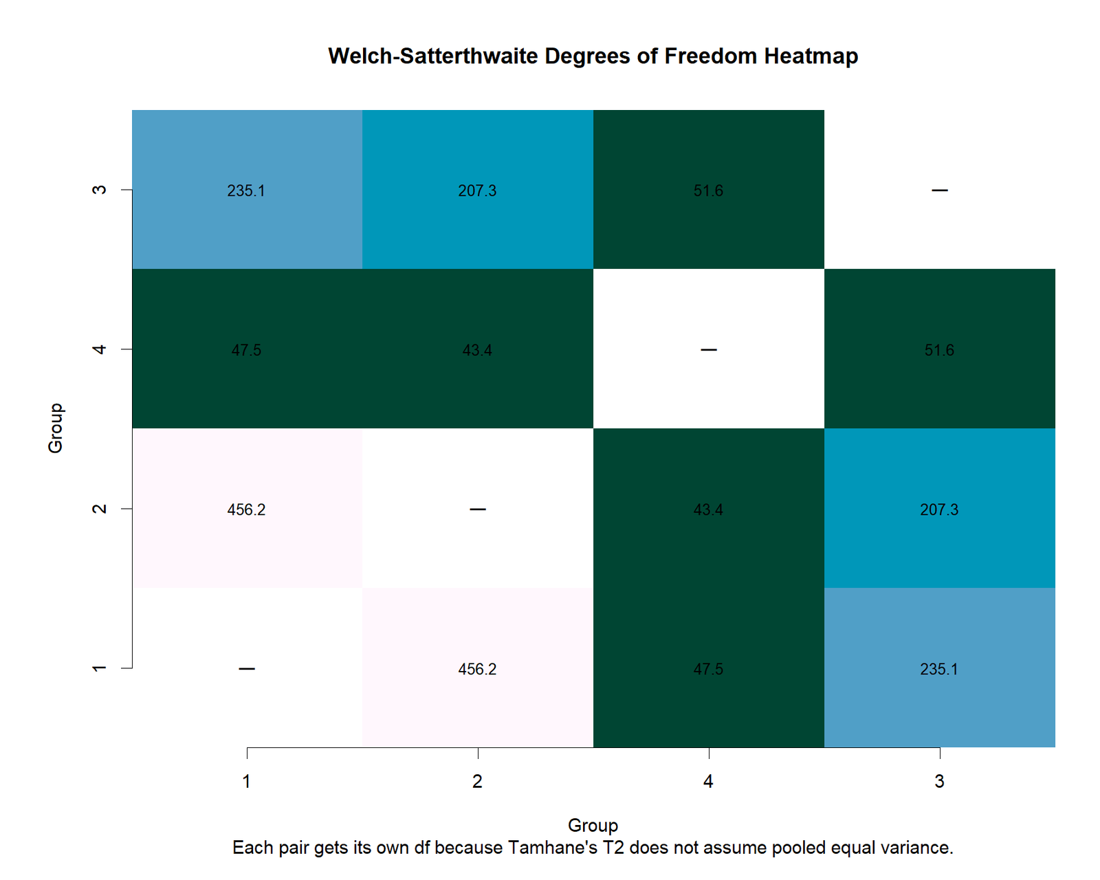
The R degrees-of-freedom heatmap confirms that Tamhane’s T2 comparisons do not all use the same error structure. Some pairs have high degrees of freedom, while pairs involving the smallest group have lower degrees of freedom.
This visual helps readers understand why unequal-variance post hoc tests are more flexible than ordinary pooled-variance procedures. Each pair is evaluated according to its own variance and sample-size information.
R Chart 8: Method Report Card
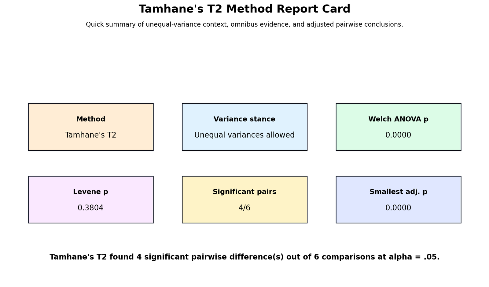
The R method report card confirms the full analysis summary. It matches the Python output: the dependent variable is G3, the grouping factor is studytime, the method is an unequal-variance Tamhane-style post hoc test, and four pairwise comparisons are significant.
The agreement between Python and R gives confidence that the published interpretation is stable across software workflows.
SPSS, R, Python and Excel Workflows for Tamhane’s T2
You can run the Tamhane T2 test in SPSS, R, Python and Excel. SPSS provides the most direct menu workflow for students. R and Python are best for reproducible charts and automation. Excel can be used for a transparent manual calculation when the sample sizes, means and variances are already known.
SPSS Workflow
| Step | SPSS Action | Purpose |
|---|---|---|
| Open data | File > Open > Data | Load the dataset containing G3 and studytime. |
| Start one-way ANOVA | Analyze > Compare Means > One-Way ANOVA | Prepare the omnibus and post hoc analysis. |
| Set dependent variable | Move G3 to Dependent List | G3 is the continuous outcome variable. |
| Set factor | Move studytime to Factor | Studytime creates the four independent groups. |
| Options | Select Descriptive, Homogeneity of variance test and Welch | Get group means, Levene test and robust omnibus test. |
| Post hoc | Select Tamhane’s T2 from the post hoc list, or use syntax /POSTHOC = T2 | Run unequal-variance pairwise comparisons. |
| Report | Export output as PDF | Save the table for verification and publication. |
R Workflow
| Step | R Action | Purpose |
|---|---|---|
| Read data | read.csv() | Load the dataset into R. |
| Prepare factor | factor(studytime) | Make sure studytime is treated as a group variable. |
| Descriptives | aggregate() or dplyr::summarise() | Calculate n, mean, standard deviation and variance. |
| Welch ANOVA | oneway.test(G3 ~ studytime, var.equal = FALSE) | Run a robust omnibus mean comparison. |
| Pairwise tests | Welch pairwise t tests with Sidak/Tamhane-style adjustment | Compare all group pairs without pooling variances. |
| Charts | ggplot2 | Create publication-ready visual output. |
Python Workflow
| Step | Python Action | Purpose |
|---|---|---|
| Read data | pandas.read_csv() | Load the dataset. |
| Group summary | groupby() | Calculate n, mean, variance and standard error by group. |
| Welch context | Use Welch ANOVA function or manual calculation | Check overall group difference under unequal-variance logic. |
| Pairwise testing | Loop through combinations of groups | Calculate pairwise mean differences, Welch SE, df, t statistic and p value. |
| Multiple adjustment | Sidak adjusted p value | Control familywise error across all six comparisons. |
| Charts | matplotlib | Export visual summaries for WordPress. |
Excel Workflow
Excel can calculate a transparent Tamhane-style comparison when you already have the group means, variances and sample sizes. For each pair, calculate the mean difference, the unequal-variance standard error, Welch degrees of freedom, the two-sided p value and an adjusted p value. Excel is helpful for teaching because students can see exactly how each pairwise result is built.
| Excel Column | Formula Idea | Meaning |
|---|---|---|
| Mean difference | =ABS(mean1-mean2) | Absolute difference between two group means. |
| Welch SE | =SQRT(var1/n1+var2/n2) | Unequal-variance standard error. |
| t statistic | =mean_difference/SE | Pairwise test statistic. |
| Welch df | Welch-Satterthwaite formula | Pair-specific degrees of freedom. |
| Unadjusted p | =T.DIST.2T(t,df) | Two-sided p value before multiple-comparison adjustment. |
| Sidak adjusted p | =1-(1-p)^m | Adjusted p value for m pairwise comparisons. |
Code Blocks for Tamhane’s T2
Corrected SPSS Syntax
* Tamhane's T2 post hoc test in SPSS One-Way ANOVA.
* Use T2 on the POSTHOC subcommand.

ONEWAY G3 BY studytime
/STATISTICS DESCRIPTIVES HOMOGENEITY WELCH
/MISSING ANALYSIS
/POSTHOC = T2 ALPHA(0.05).

OUTPUT EXPORT
/CONTENTS EXPORT=ALL
/PDF DOCUMENTFILE='D:\DATA ANALYSIS\F Post Hoc Tests\Tamhanes T2\SPSS_Output\Tamhanes-T2-SPSS-Output.pdf'.
Python Skeleton
import pandas as pd
import numpy as np
from itertools import combinations
from scipy import stats

df = pd.read_csv("dataset.csv")
df = df[["G3", "studytime"]].dropna()
df["studytime"] = df["studytime"].astype(int)

summary = df.groupby("studytime")["G3"].agg(["count", "mean", "std", "var"])
pairs = []
m = len(list(combinations(summary.index, 2)))

for g1, g2 in combinations(summary.index, 2):
n1, n2 = summary.loc[g1, "count"], summary.loc[g2, "count"]
mean1, mean2 = summary.loc[g1, "mean"], summary.loc[g2, "mean"]
var1, var2 = summary.loc[g1, "var"], summary.loc[g2, "var"]

```
se = np.sqrt(var1 / n1 + var2 / n2)
diff = abs(mean1 - mean2)

df_welch = (var1/n1 + var2/n2)**2 / (
    ((var1/n1)**2 / (n1 - 1)) + ((var2/n2)**2 / (n2 - 1))
)

t_value = diff / se
p_unadjusted = 2 * stats.t.sf(t_value, df_welch)
p_sidak = 1 - (1 - p_unadjusted) ** m

pairs.append({
    "group_1": g1,
    "group_2": g2,
    "mean_difference": diff,
    "welch_se": se,
    "welch_df": df_welch,
    "t": t_value,
    "p_unadjusted": p_unadjusted,
    "p_sidak_adjusted": min(p_sidak, 1.0),
    "decision": "Significant" if p_sidak < .05 else "Not significant"
})
```

pairwise_table = pd.DataFrame(pairs)
print(summary)
print(pairwise_table)
R Skeleton
df <- read.csv("dataset.csv")
df <- na.omit(df[, c("G3", "studytime")])
df$studytime <- factor(df$studytime)

aggregate(G3 ~ studytime, data = df, function(x) {
c(n = length(x), mean = mean(x), sd = sd(x), var = var(x))
})

welch_result <- oneway.test(G3 ~ studytime, data = df, var.equal = FALSE)
print(welch_result)

groups <- levels(df$studytime)
m <- choose(length(groups), 2)
results <- data.frame()

for(i in 1:(length(groups)-1)){
for(j in (i+1):length(groups)){
x <- df$G3[df$studytime == groups[i]]
y <- df$G3[df$studytime == groups[j]]

```
n1 <- length(x); n2 <- length(y)
v1 <- var(x); v2 <- var(y)
se <- sqrt(v1/n1 + v2/n2)
diff <- abs(mean(x) - mean(y))

df_welch <- (v1/n1 + v2/n2)^2 / (((v1/n1)^2/(n1-1)) + ((v2/n2)^2/(n2-1)))
t_value <- diff / se
p_unadj <- 2 * pt(-abs(t_value), df_welch)
p_sidak <- 1 - (1 - p_unadj)^m

results <- rbind(results, data.frame(
  group_1 = groups[i],
  group_2 = groups[j],
  mean_difference = diff,
  welch_se = se,
  welch_df = df_welch,
  t = t_value,
  p_unadjusted = p_unadj,
  p_sidak_adjusted = min(p_sidak, 1),
  decision = ifelse(p_sidak < .05, "Significant", "Not significant")
))
```

}
}

print(results)
Excel Pairwise Formula Example
Mean Difference:
=ABS(B2-B3)

Welch Standard Error:
=SQRT(D2/C2 + D3/C3)

Welch t Statistic:
=E2/F2

Welch Degrees of Freedom:
=(D2/C2 + D3/C3)^2 / (((D2/C2)^2/(C2-1)) + ((D3/C3)^2/(C3-1)))

Two-Sided p Value:
=T.DIST.2T(G2,H2)

Sidak Adjusted p Value:
=1-(1-I2)^6
APA Reporting Wording for Tamhane’s T2
APA-style result: A one-way comparison was conducted to examine whether final grade differed across weekly studytime groups. The Welch robust test was significant, F(3, 139.10) = 18.18, p < .001. Because pairwise comparisons were required under an unequal-variance post hoc framework, Tamhane’s T2-style comparisons were examined.
Tamhane’s T2 indicated that the <2 hours group had significantly lower G3 scores than the 2 to 5 hours group, mean difference = 1.25, adjusted p = .000115, the 5 to 10 hours group, mean difference = 2.38, adjusted p < .001, and the >10 hours group, mean difference = 2.21, adjusted p = .00151. The 2 to 5 hours group also scored significantly lower than the 5 to 10 hours group, mean difference = 1.14, adjusted p = .00233. The remaining two comparisons were not significant after adjustment.
Plain-language version: Students who studied less than 2 hours per week had lower final grades than students who studied more. The best-performing group was 5 to 10 hours, but this group was not significantly different from the >10 hours group after adjustment.
Common Mistakes When Using Tamhane’s T2
Mistake 1: Using Tamhane’s T2 for only two groups
Tamhane’s T2 is a post hoc multiple comparison procedure. If there are only two independent groups, use a standard independent samples t test or Welch’s t test instead.
Mistake 2: Reporting only the ANOVA p value
The omnibus ANOVA or Welch ANOVA tells whether there is an overall mean difference, but it does not identify which groups differ. A complete report must include pairwise comparisons.
Mistake 3: Ignoring adjusted p values
Post hoc tests involve multiple comparisons. Reporting unadjusted p values can inflate Type I error. Use the adjusted p values or adjusted confidence intervals for final decisions.
Mistake 4: Saying non-significant means “equal”
A non-significant Tamhane comparison means the analysis did not detect a statistically reliable difference after adjustment. It does not prove that the two group means are exactly equal.
Mistake 5: Using the wrong SPSS syntax keyword
In SPSS syntax, the Tamhane’s T2 post hoc option is commonly written as T2 on the POSTHOC subcommand. Writing TAMHANE may produce a syntax error in the One-Way ANOVA command.
Downloads and Resources
Use these resources to verify the Tamhane’s T2 workflow, charts and output. The Python and R reports contain the reproducible post hoc tables and visual summaries. The SPSS output contains the group descriptives, homogeneity context, classic ANOVA, Welch robust test and visual context.
Download Python Report
Tamhane’s T2 Python output with group summaries, Welch context and pairwise comparisons.
Download R Report
R validation report with matching unequal-variance post hoc results and charts.
Download SPSS Output
SPSS output for descriptives, Levene context, Welch ANOVA and visual group summary.
Copy Code Blocks
Use the SPSS, Python, R and Excel code sections in this guide.
FAQs About Tamhane’s T2
What is Tamhane’s T2 test?
Tamhane’s T2 is an unequal-variance post hoc test used to compare group means pair by pair after an ANOVA or Welch ANOVA. It is designed for situations where equal variances are not assumed.
When should I use Tamhane T2 instead of Tukey?
Use Tamhane T2 when variances or sample sizes are unequal and you want a conservative unequal-variance post hoc test. Tukey is more suitable when the equal-variance assumption is reasonable.
What does “Tamhane’s T2 variances not assumed” mean?
It means the pairwise comparisons do not rely on the assumption that all groups have the same variance. Each pair uses unequal-variance standard error logic.
How do I run Tamhane’s T2 in SPSS?
Use Analyze > Compare Means > One-Way ANOVA, place the continuous outcome in the dependent list, place the group variable as the factor, choose post hoc tests, and select Tamhane’s T2. In syntax, use /POSTHOC = T2 ALPHA(.05).
What was the result in this Tamhane’s T2 example?
The Welch ANOVA was significant, and Tamhane-style pairwise tests found four significant comparisons out of six. The <2 hours studytime group had significantly lower G3 scores than the other studytime groups.
Can I run Tamhane T2 in Python?
Yes. Python can reproduce a Tamhane-style unequal-variance post hoc workflow by calculating pairwise mean differences, Welch standard errors, Welch degrees of freedom and adjusted p values.
Can I calculate Tamhane’s T2 in Excel?
Excel can calculate a transparent approximation using group means, variances, sample sizes, Welch standard errors, Welch degrees of freedom and adjusted p values. For official reporting, software such as SPSS, R or Python is preferred.
Is Tamhane’s T2 the same as Games-Howell?
No. Both are unequal-variance post hoc methods, but they use different adjustment logic. Games-Howell is also popular after Welch ANOVA, while Tamhane’s T2 is often described as more conservative.

