
Nonparametric Tests in R: 12 Essential Methods, Code and Interpretation
Nonparametric tests in R help answer research questions about ranks, medians, paired differences, several-group comparisons, monotonic association, distributional differences and exact probabilities without forcing every problem into one normal-theory template. This R-only guide shows how to choose the right method, check assumptions, run practical base-R workflows, interpret effect sizes, and report a verified Kruskal–Wallis example with Benjamini–Hochberg pairwise follow-up testing.
The correct nonparametric test in R depends on design, dependence and the question being asked.
Nonparametric tests in R are not a single interchangeable category for “non-normal data.” A Wilcoxon rank-sum test addresses a two-independent-group ordering question; a Wilcoxon signed-rank test evaluates paired differences; a Kruskal–Wallis test compares several independent groups; a Friedman test handles repeated conditions; Spearman and Kendall address monotonic association; and exact or permutation procedures let the statistic define the null question directly.
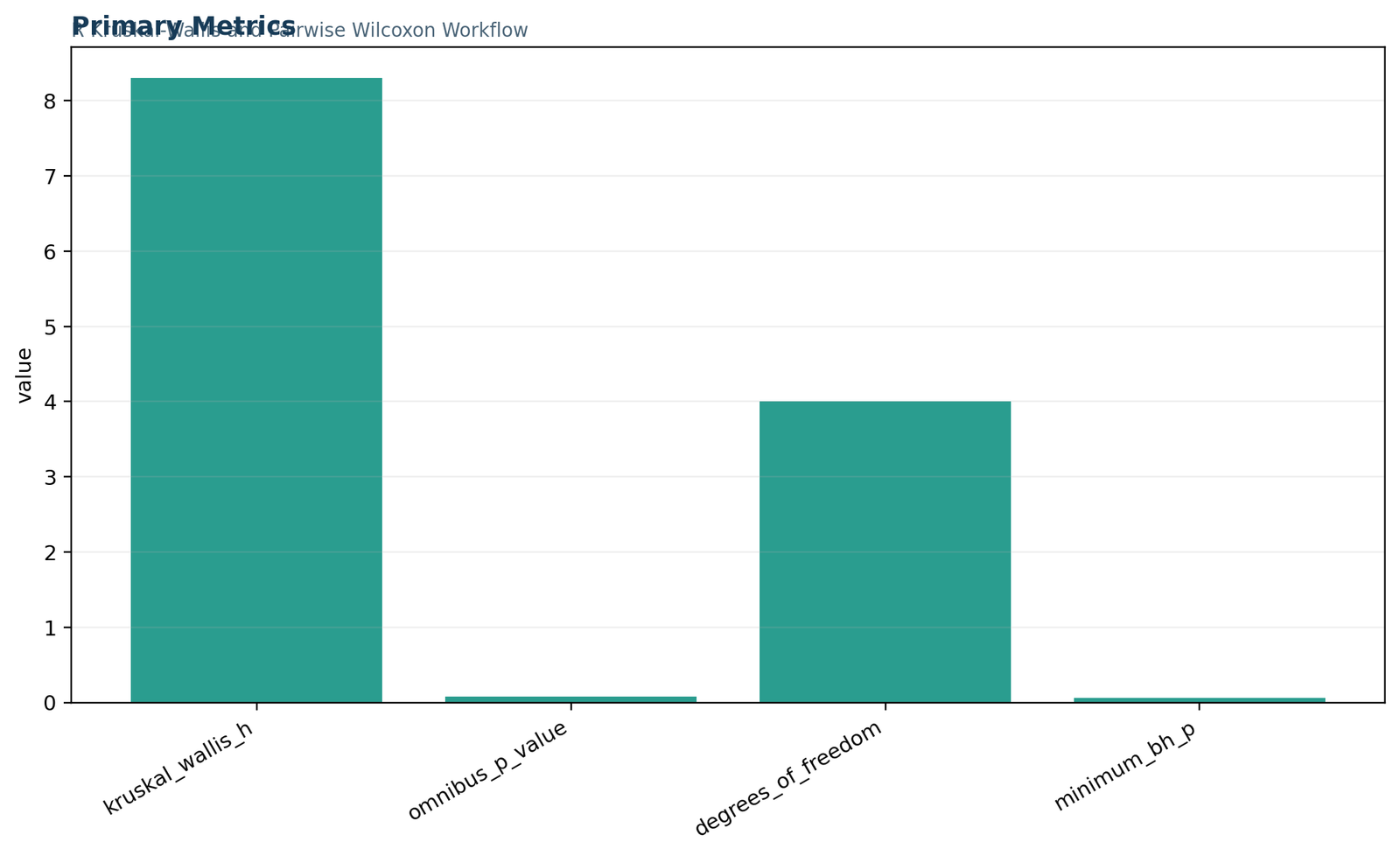
In the verified R-only example, student absences were compared across five levels of maternal job status (Mjob: at_home, health, other, services and teacher). The tie-corrected Kruskal–Wallis statistic was H = 8.300399 with df = 4 and p = 0.081174, so the omnibus result was not statistically significant at α = .05. Benjamini–Hochberg adjusted pairwise Wilcoxon follow-ups likewise produced no adjusted discoveries; the smallest adjusted p-value was approximately 0.0605 for health versus services.
What are nonparametric tests in R?
Methods that base inference on order, ranks, signs, exact counts or resampled statistics rather than one narrow normal-theory template.
Nonparametric tests in R are best selected by their inferential target. Some compare ordered observations across independent groups, some analyze paired differences, some compare entire empirical distributions, some estimate monotonic association, and some use randomization or exact enumeration to calculate p-values from a user-defined statistic.
What “nonparametric” means in practice
In practice, nonparametric tests in R reduce dependence on a fully specified distributional model. They often work well when outcomes are ordinal, skewed, heavy-tailed, outlier-prone, zero-inflated or naturally understood through ordering rather than means. The attraction is not that they are assumption-free. The attraction is that the method can align more directly with the question: do paired differences center on zero, do several groups share the same distribution, or does one group tend to have larger observations than another?
R is especially convenient because many standard procedures are available in base functions such as wilcox.test(), kruskal.test(), friedman.test(), cor.test(), ks.test() and fisher.test(). Additional packages extend the toolbox, but an R-only article can still teach the core logic using reproducible base-R workflows.
What “nonparametric” does not mean
It does not mean that every rank procedure is a median test. Mann–Whitney and Kruskal–Wallis are naturally distribution-sensitive rank tests. A median-shift interpretation usually requires comparable group shapes. Likewise, the Wilcoxon signed-rank test is not a generic paired test of means; it targets the distribution of paired differences and needs a reasonable symmetry condition for a clean location interpretation.
It also does not mean that parametric methods should be abandoned whenever a normality test rejects. Large samples detect trivial deviations, while many mean-based models remain robust. Good analysis starts with design, target parameter and data scale—not with a single assumption test performed after the fact.
For foundational context, see parametric vs nonparametric tests, null and alternative hypotheses and p-value interpretation.
Why this topic matters in applied work
Many real datasets are not well behaved from a textbook perspective. Count outcomes pile up at zero, rating scales have only a few ordered categories, and educational or clinical variables often show skew, ceiling effects or long right tails. In those settings, nonparametric tests in R help analysts keep the inference aligned with what the data can actually support. Instead of forcing the discussion to revolve around means and standard deviations alone, the workflow can emphasize medians, IQRs, rank order, stochastic dominance and direct randomization logic.
That practical flexibility is one reason nonparametric tests in R remain so widely used. They are not a fallback for bad data. They are often the most natural first choice when the measurement scale, design or research target is rank-oriented from the beginning. A survey item with five ordered categories, a satisfaction score, a symptom count, a reaction-time measure with severe skew, or a pretest/posttest difference with many small changes can all motivate nonparametric reasoning long before any normality discussion begins.
What makes R especially useful here
R is strong for nonparametric work because it combines concise function calls with transparent objects, easy tabulation, formula interfaces and strong visualization support. Even when using only base R, an analyst can read the data, clean variables, compute descriptives, run the test, format pairwise comparisons and export results in a compact script. That matters for reproducibility because the full path from raw data to interpretation can stay in a single auditable file.
Another strength is that nonparametric tests in R are easy to combine with custom helper calculations. If a built-in function reports the main statistic but not the effect size you want, the ranks and sample sizes can usually be used to calculate that effect explicitly. This article follows that spirit by pairing the built-in test calls with visibly stated effect-size and multiplicity logic.
How to choose nonparametric tests in R
A design-first framework prevents the common mistake of treating all rank tests as interchangeable.
Choosing nonparametric tests in R begins with four questions: Are the observations independent or paired? How many groups or conditions exist? Is the target location, distribution, scale or association? Is the outcome ordered, counted or nominal?
| Design and question | Primary R method | Base R function | What it answers | Main caution |
|---|---|---|---|---|
| Two independent groups | Wilcoxon rank-sum / Mann–Whitney | wilcox.test(x, y) | Whether one group tends to have larger observations. | A median-shift interpretation needs similar shapes. |
| Two paired measurements | Wilcoxon signed-rank | wilcox.test(x, y, paired = TRUE) | Whether paired differences are centered around zero. | Zeros and asymmetry affect interpretation. |
| Several independent groups | Kruskal–Wallis | kruskal.test(y ~ g) | Whether at least one group distribution differs. | Post-hoc tests are needed for localization. |
| Repeated conditions | Friedman test | friedman.test(y ~ condition | id) | Whether repeated-condition distributions differ. | Data must be blocked by subject or unit. |
| Monotonic association | Spearman or Kendall | cor.test(x, y, method = "spearman") | Strength of monotonic association. | Association is not causation. |
| Entire distribution difference | Two-sample Kolmogorov–Smirnov | ks.test(x, y) | Largest gap between two ECDFs. | Ties complicate exact interpretation. |
| Small categorical tables | Fisher’s exact test | fisher.test(tab) | Exact association in contingency tables. | Targets counts, not ranks. |
A fast decision checklist
Ask these questions in order. First, are the observations independent or paired? Second, is the outcome at least ordinal? Third, how many groups or conditions are involved? Fourth, do you care about a shift in ordering, a direct median difference, the entire distribution, monotonic association or exact probabilities in counts? Fifth, will you need follow-up comparisons, and if so, how will you control multiplicity?
Answering those questions usually narrows the choice quickly. Two independent groups with an ordinal outcome suggest rank-sum testing. Two measurements on the same unit suggest a signed-rank or sign procedure. Several independent groups suggest Kruskal–Wallis. Several repeated conditions suggest Friedman. If none of those standard templates matches the question closely, a permutation workflow can often be built around the exact statistic of interest.
Why generic rules fail
A common but weak rule says, “If the data are not normal, use a nonparametric test.” That rule fails because it ignores design. The correct comparison for paired observations is still paired even if the data are normal, skewed or ordinal. The correct comparison for repeated conditions still requires blocking. Likewise, replacing a targeted permutation test of medians with a rank-sum test changes the scientific question, even when both procedures are called nonparametric.
In other words, nonparametric tests in R are best viewed as a family of tools, not a single emergency option. Better-than-competitor explanations make that explicit so that readers know why one method answers their question and another does not.
Assumptions for nonparametric tests in R
Nonparametric does not mean assumption-free; it means the assumptions are different and often closer to design and ordering.
The practical validity of nonparametric tests in R depends on independence, correct pairing, an orderable outcome, transparent treatment of ties and a clear match between the method and the research question.
Independence or correct pairing
Independent-group methods require independent units. Paired methods require one clearly matched record per unit in each condition. Using the wrong structure distorts p-values and effect sizes.
Ordered outcome
Most rank methods require at least ordinal data. Nominal outcomes call for categorical procedures such as exact tests, chi-square methods or agreement statistics instead.
Tie transparency
Discrete outcomes create ties. R may use exact, normal-approximation or continuity-corrected calculations depending on sample size and ties. Report the method rather than assuming all p-values are identical.
Comparable shape when claiming medians
Kruskal–Wallis and rank-sum procedures compare rank distributions. Concluding that medians differ requires the groups to have similarly shaped distributions.
Symmetry for signed-rank interpretation
The Wilcoxon signed-rank test assumes the paired-difference distribution is reasonably symmetric when interpreted as a location shift test. If that is doubtful, the sign test is a safer fallback.
Planned multiplicity control
When several pairwise comparisons follow an omnibus test, the adjustment method should be decided in advance. This article uses Benjamini–Hochberg control for the family of pairwise Wilcoxon tests.
How to check assumptions in practice
Assumption checking should be descriptive and design-based, not a ritual of running one more hypothesis test. Inspect group sizes, missingness, the presence of structural zeros, duplicated values, and whether the ordering of the outcome makes substantive sense. For paired procedures, verify that each unit contributes one value per condition and that the matching is meaningful rather than accidental. For independent-group procedures, confirm that no clustering or repeated observations are hiding inside the sample.
The more discrete the outcome, the more ties you should expect. That does not invalidate nonparametric tests in R, but it does affect exactness and may change whether a normal approximation is used. Transparent reporting should therefore mention ties, especially for count variables like the absences example in this article.
What assumptions are often overstated
Readers often hear that nonparametric tests have “no assumptions.” The more accurate statement is that they usually make fewer or different distributional assumptions. They still assume meaningful sampling units, correctly specified dependence, and a test that matches the outcome scale. A rank correlation between two variables is still meaningless if one variable was miscoded or if the sampling design makes the observations dependent in an unrecognized way.
The practical value of nonparametric tests in R comes from being honest about these assumptions rather than pretending they do not exist. That honesty improves interpretation and reduces the temptation to overstate what a significant or non-significant result means.
options(stringsAsFactors = FALSE)
alpha <- 0.05student <- read.csv("student-por.csv", sep = ";")
needed <- c("absences", "Mjob")
missing <- setdiff(needed, names(student))
if (length(missing) > 0) stop(paste("Missing columns:", paste(missing, collapse = ", ")))
analysis <- subset(student, !is.na(absences) & !is.na(Mjob), select = c(absences, Mjob))
analysis$Mjob <- factor(analysis$Mjob,
levels = c("at_home", "health", "other", "services", "teacher"))
stopifnot(nrow(analysis) == 649)
stopifnot(nlevels(analysis$Mjob) == 5)
R setup, data cleaning and reproducibility
A dependable workflow records the exact variables, factor levels, exclusions and multiplicity plan before inference begins.
A production workflow for nonparametric tests in R should validate columns, fix the intended factor order, preserve the raw values, and make the analysis script auditable. R’s defaults are powerful, but being explicit reduces the risk of hidden recoding or accidental reordering.
Why data validation matters
If the grouping variable contains spelling variants, stray blanks or unexpected levels, a group comparison can silently become a six-group analysis instead of a five-group analysis. Converting the grouping variable to a factor with fixed levels makes the workflow explicit and stabilizes tables, plots and pairwise output ordering.
For nonparametric tests in R, especially those based on ranks, it is equally important to preserve the raw measurement scale. Never pre-rank values manually unless the method requires it and the audit trail documents every step.
Reproducibility checklist
Recommended file structure
A durable analysis project benefits from a simple structure: one folder for raw data, one for cleaned or analysis-ready data, one for scripts, one for output tables and one for charts. Even when a single post is being created, this separation helps keep nonparametric tests in R auditable. The raw file remains untouched, the analysis script becomes the canonical record of cleaning decisions, and the output folder preserves the charts and reports used in the article.
When the article is later updated, that organization makes it easier to regenerate the entire workflow consistently. It also prevents a common failure mode in content production: a chart is updated but the narrative or downloadable report is left behind.
Version control and comment style
R scripts become much easier to trust when each major step is labeled: import, validation, descriptives, omnibus test, pairwise follow-up, effect sizes and reporting tables. Short comments describing why a step exists are more useful than decorative comments that repeat the code. If a method choice is not obvious, a brief comment documenting the rationale—for example, “BH adjustment selected to control false-discovery rate across ten pairwise comparisons”—greatly improves transparency.
That style also makes nonparametric tests in R easier to teach. Readers can see the analysis not merely as a set of function calls but as a sequence of decisions.
Worked example: R Kruskal–Wallis and BH-adjusted pairwise Wilcoxon tests
A practical several-group comparison of student absences across maternal-job categories.
This verified example for nonparametric tests in R evaluates whether absence distributions differ across five maternal-occupation groups. The omnibus test is Kruskal–Wallis, followed by pairwise Wilcoxon rank-sum tests with Benjamini–Hochberg adjustment as a planned follow-up layer.
Research question and hypotheses
Question: Do student absence distributions differ across the five Mjob groups?
Under the Kruskal–Wallis framework, the groups share the same population distribution under the null.
The omnibus test indicates whether a distributional difference is present somewhere among the five groups; it does not identify the differing pairs by itself.
Variables and group counts
| Group | n | Mean rank | Rank sum |
|---|---|---|---|
| at_home | 135 | 324.3296 | 43,784.5 |
| health | 48 | 267.0521 | 12,818.5 |
| other | 258 | 327.7791 | 84,567.0 |
| services | 136 | 350.3456 | 47,647.0 |
| teacher | 72 | 307.0556 | 22,108.0 |
| Mjob group | n | Mean | SD | Median | Q1 | Q3 | IQR | Range |
|---|---|---|---|---|---|---|---|---|
| at_home | 135 | 3.5704 | 4.3530 | 2.0 | 0.0 | 6.0 | 6.0 | 0–21 |
| health | 48 | 2.1042 | 2.7617 | 1.5 | 0.0 | 4.0 | 4.0 | 0–10 |
| other | 258 | 3.8101 | 4.8949 | 2.0 | 0.0 | 6.0 | 6.0 | 0–32 |
| services | 136 | 4.3015 | 5.1501 | 2.0 | 0.0 | 6.0 | 6.0 | 0–30 |
| teacher | 72 | 3.1111 | 3.9702 | 2.0 | 0.0 | 4.25 | 4.25 | 0–18 |
Why this example is useful
This example is realistic because it combines several features that appear frequently in applied work: a discrete count outcome, multiple groups with unequal sample sizes, many ties, and a need for follow-up comparisons that should not be interpreted without adjustment. Those properties make it much richer than a toy example where each group is tiny and all values are distinct.
For readers trying to learn nonparametric tests in R, that realism matters. It shows not only how to run the function, but also how to think about group summaries, tie correction, effect size and multiplicity in one coherent workflow.
What the descriptives already suggest
Before any test is run, the descriptive statistics reveal that the groups are not identical in a simple visual sense. The services group has the largest mean and highest mean rank, while the health group has the smallest. Yet the group medians remain close, and the distributions overlap substantially. That is exactly the sort of situation where an omnibus rank test may be suggestive without becoming conventionally significant.
Stated differently, the example helps separate descriptive contrast from inferential certainty. Good articles about nonparametric tests in R should teach that separation clearly.
kw <- kruskal.test(absences ~ Mjob, data = analysis)
kwpairwise_bh <- pairwise.wilcox.test(
x = analysis$absences,
g = analysis$Mjob,
p.adjust.method = "BH",
exact = FALSE
)
pairwise_bh
# Small-sample effect size often reported with Kruskal-Wallis
n <- nrow(analysis)
k <- nlevels(analysis$Mjob)
epsilon_sq <- max((unname(kw$statistic) - k + 1) / (n - k), 0)
epsilon_sq
Kruskal–Wallis formula, tie correction and verified result
The omnibus statistic is calculated from pooled ranks and then corrected for ties because absences is a discrete count variable.
The worked nonparametric tests in R analysis uses a tie-corrected Kruskal–Wallis statistic because many students share the same absence counts. The visible workbook formulas confirm the pooled-rank result rather than relying on software output alone.
Here, Rj is the rank sum for group j, nj is the group size, k = 5, and N = 649. Because the absence variable contains repeated values, the uncorrected statistic is divided by the tie-correction factor.
Verified omnibus calculation
Pairwise BH summary
Two raw pairwise p-values fell below .05, but neither remained below .05 after Benjamini–Hochberg adjustment. That is exactly why multiple-testing control needs to be specified before interpreting pairwise rank tests.
| Comparison | U statistic | Raw p-value | BH-adjusted p | BH decision |
|---|---|---|---|---|
| health vs services | 2,418.5 | 0.006047 | 0.060467 | Not significant |
| health vs other | 5,035.5 | 0.033502 | 0.167512 | Not significant |
| at_home vs health | 3,809.5 | 0.060177 | 0.200591 | Not significant |
| services vs teacher | 5,553.5 | 0.101891 | 0.254728 | Not significant |
| at_home vs services | 8,437.0 | 0.236857 | 0.358663 | Not significant |
| health vs teacher | 1,518.0 | 0.237996 | 0.358663 | Not significant |
| other vs services | 16,343.0 | 0.251064 | 0.358663 | Not significant |
| other vs teacher | 9,881.5 | 0.392065 | 0.490081 | Not significant |
| at_home vs teacher | 5,111.0 | 0.526849 | 0.585388 | Not significant |
| at_home vs other | 17,247.0 | 0.871622 | 0.871622 | Not significant |
Why tie correction matters here
The absences variable contains many repeated values, especially zero, small integers and shared mid-range counts. Because Kruskal–Wallis is based on pooled ranks, those ties affect the theoretical variance of the rank sums. Ignoring that fact would slightly distort the omnibus statistic. The workbook therefore makes the tie correction explicit, and the reported H = 8.300399 is the corrected value rather than the uncorrected H = 7.788148.
This is an important educational point because readers sometimes assume software output is a black box. In reality, the correction can be verified directly, and doing so builds trust in the result.
How to interpret the near-threshold pattern
An omnibus p-value of 0.081174 is not conventionally significant at α = .05, but it is close enough to invite careful descriptive interpretation. The correct response is not to relabel it as “marginally significant” and certainly not to cherry-pick the smallest pairwise raw p-values. The correct response is to state that the evidence is suggestive but insufficient under the planned threshold and then to show that the BH-adjusted pairwise comparisons are consistent with that conclusion.
That combination—moderate descriptive variation, a non-significant omnibus p-value and no adjusted pairwise discoveries—is common in practice and is worth understanding well if you want to use nonparametric tests in R responsibly.
R charts for the verified nonparametric workflow
The charts summarize the omnibus statistic, descriptive group structure, pairwise BH results and the final interpretation.
These R charts for nonparametric tests in R are interpreted using the verified workbook values. Chart 1 appears alone at full width; charts 2–3 form the first pair; charts 4–5 form the second pair.
Primary metrics
This full-width summary reports the core omnibus findings: N = 649, k = 5, H = 8.3004, df = 4, p = 0.0812 and epsilon squared = 0.006678. The effect-size estimate is very small, which helps explain why the visual group differences do not translate into strong inferential evidence.
Maternal-job absence summary
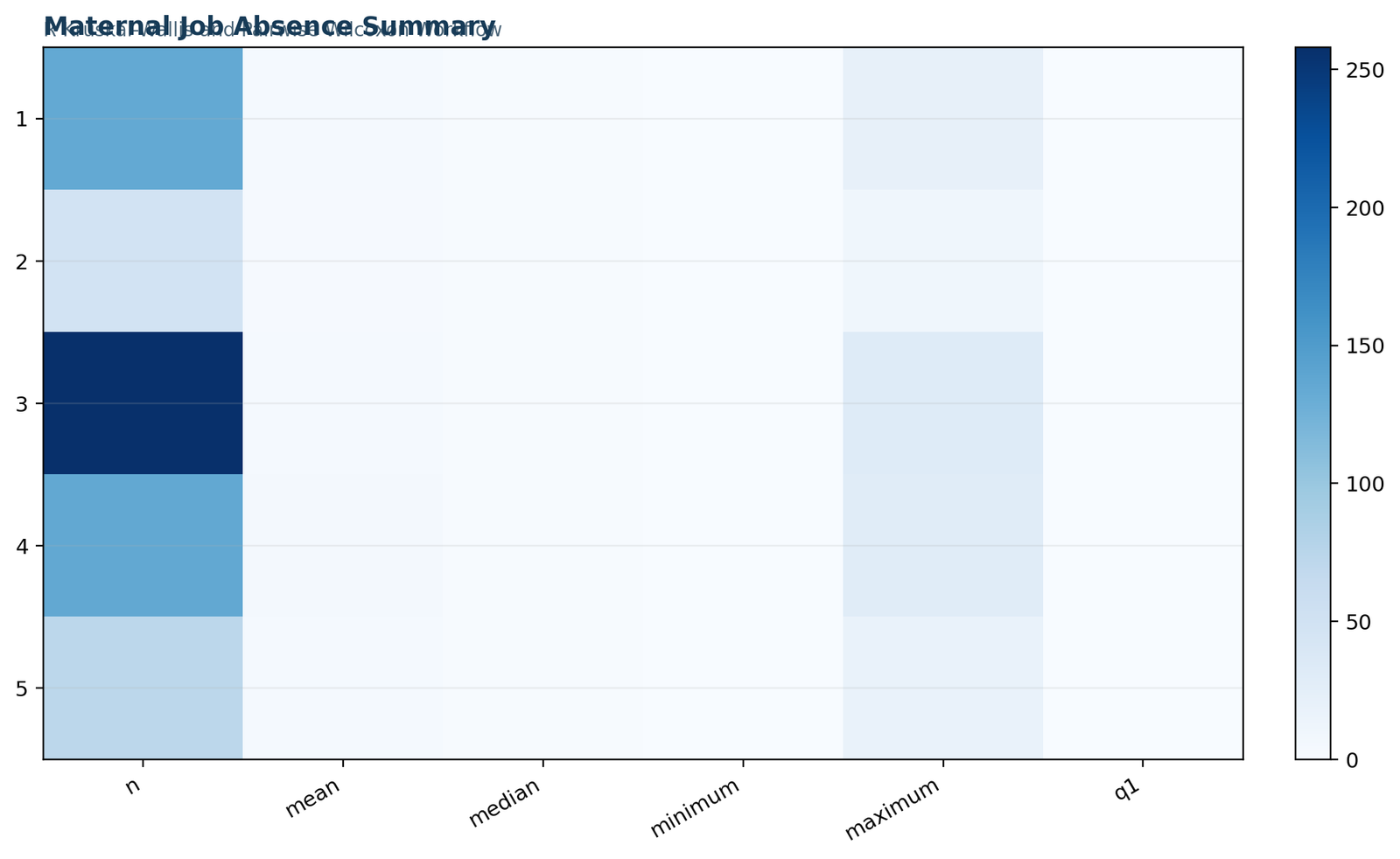
The descriptive panel shows the five groups side by side. The services group has the largest mean and mean rank, while the health group has the smallest. Medians remain relatively close, and several groups share the same IQR of 6, which is consistent with a suggestive but not decisive omnibus result.
Pairwise Wilcoxon with BH adjustment
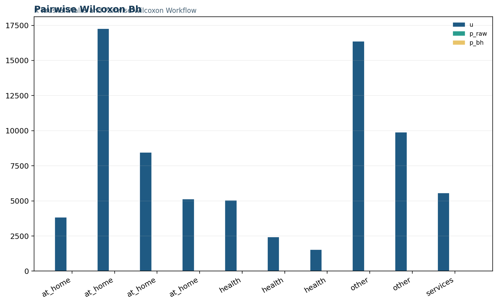
This chart visualizes the ten pairwise comparisons after Benjamini–Hochberg adjustment. The smallest adjusted p-value belongs to health versus services at about 0.0605, followed by health versus other at about 0.1675. None crosses the .05 threshold, so no adjusted pair is declared significant.
BH decision outcomes
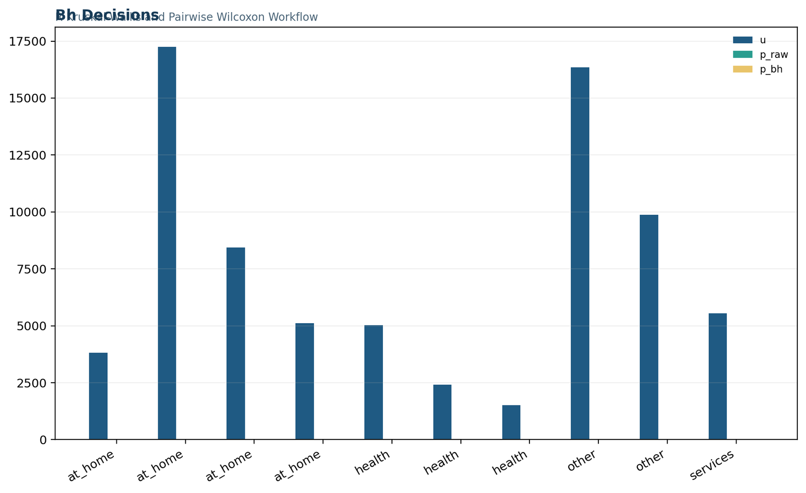
The decision chart shows the practical impact of multiplicity control: although some raw pairwise p-values are relatively small, the planned false-discovery-rate adjustment keeps every comparison in the non-significant region. This is a useful reminder that post-hoc interpretation should be based on the adjusted results, not the raw p-values alone.
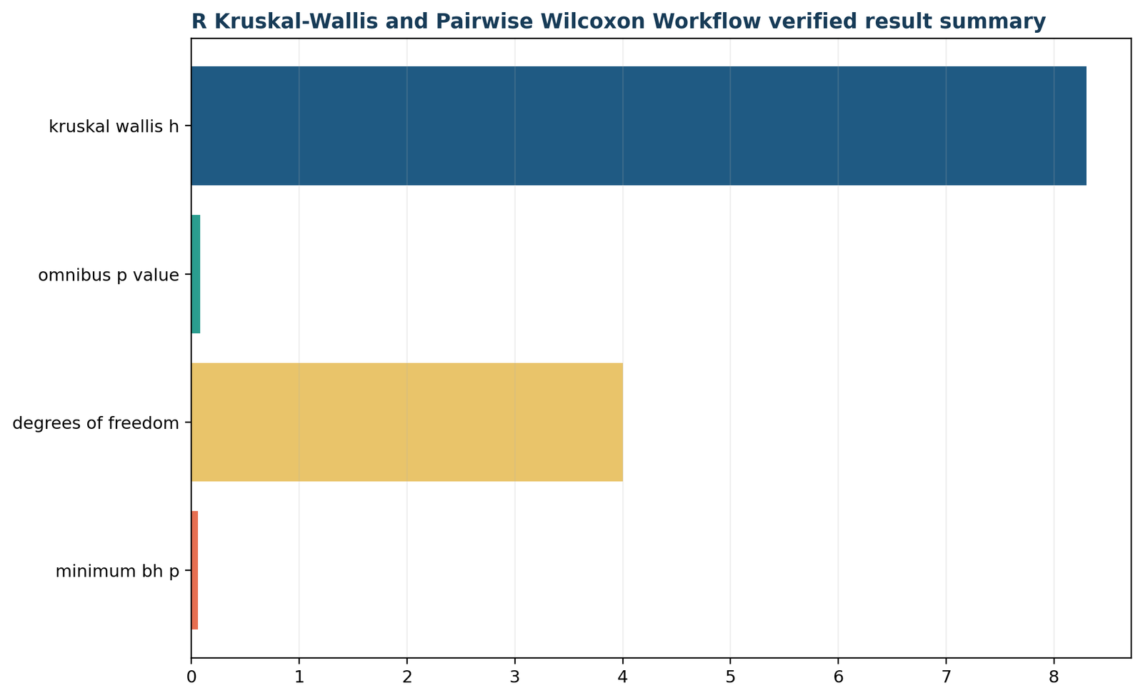
Verified result summary
The closing R summary reconciles the workbook and scripted analysis. It confirms the tie-corrected omnibus result, the very small effect size, and the absence of any BH-significant pairwise comparisons. That consistency across descriptive tables, omnibus testing and follow-up testing is exactly what a high-quality nonparametric workflow should provide.
Independent-sample nonparametric tests in R
When two groups are independent, the most common R choice is the Wilcoxon rank-sum / Mann–Whitney procedure.
For two independent groups, nonparametric tests in R usually begin with wilcox.test(). The null is often phrased as no shift in distribution or no tendency for one group to produce larger values than the other.
x <- subset(student, school == "GP")$G1

y <- subset(student, school == "MS")$G1

fit <- wilcox.test(x, y,

alternative = "two.sided",

exact = FALSE,

conf.int = TRUE)

fit
When to use it
Use the rank-sum test when you have two independent groups and an ordinal or continuous outcome that is not well summarized by a mean-based model. It is especially attractive when the scientific interpretation concerns relative ordering or robustness to skew and outliers.
How to report it
Report the group sizes, medians, IQRs, the R test statistic, whether the p-value is exact or approximate, and an effect size such as rank-biserial correlation or probability of superiority. If you phrase the result as a median comparison, justify the comparable-shape assumption.
Rank-sum output conventions in R
R reports a statistic labeled W for the Wilcoxon rank-sum test. Other software may emphasize the Mann–Whitney U statistic instead. They are directly related, so the substantive conclusion is the same once the sample sizes are known. Good teaching material on nonparametric tests in R should warn readers about this naming difference so they are not confused when comparing software packages or textbook formulas.
It is also good practice to accompany the p-value with an effect size such as rank-biserial correlation, probability of superiority or a confidence interval for the location shift if the software version supports it.
When a direct median test may be better
Sometimes the rank-sum procedure is not the clearest choice even for two independent groups. If the research question is narrowly about the median and the analyst wants that exact null addressed, a permutation test based on the sample median may be more direct. That is why better guides to nonparametric tests in R spend time on target selection instead of treating the rank-sum test as the universal answer.
The best method is the one that answers the intended question while respecting the data structure—not merely the one that is most familiar.
Paired-sample nonparametric tests in R
Use paired methods only when each observation in one condition is meaningfully matched to one observation in another.
For paired data, nonparametric tests in R typically rely on wilcox.test(..., paired = TRUE) or, when only the direction of change matters, a sign test from an additional package or a custom exact calculation.
before <- student$G1

after  <- student$G2

paired_fit <- wilcox.test(before, after,

paired = TRUE,

alternative = "two.sided",

exact = FALSE,

conf.int = TRUE)

paired_fitSigned-rank versus sign logic
The signed-rank test uses both the sign and the rank of the absolute paired differences, so it typically has more power than the sign test when its symmetry condition is reasonable. The sign test uses only the direction of change. That makes it less informative but sometimes more robust when differences are highly skewed or when outliers dominate the magnitudes.
Readers learning nonparametric tests in R should understand this trade-off clearly. A more powerful method is not automatically a better method if its interpretation no longer matches the data-generating pattern.
Handling zeros in paired data
Paired analyses often contain zeros, meaning no observed change for some units. Different software and functions may treat zeros slightly differently depending on the method and options. Public-facing reporting should therefore state the number of zero differences when it matters and clarify how they were handled.
That level of detail is one of the features that separates a genuinely useful guide on nonparametric tests in R from a thin competitor page built only around definitions.
Several independent groups: Kruskal–Wallis and follow-up testing in R
The worked example belongs to the most common multi-group rank-testing situation.
Among nonparametric tests in R, the Kruskal–Wallis procedure is the standard extension of rank-based comparison to more than two independent groups. The post-hoc question then becomes how to localize differences while controlling multiplicity.
Omnibus stage
Start with kruskal.test() using the full set of groups. This step asks whether at least one group distribution differs. A non-significant result, like the worked example’s p = 0.081, does not prove equality, but it tells you that the evidence for a group difference is not conventionally strong.
Follow-up stage
If follow-up comparisons are planned, use pairwise Wilcoxon tests and report the adjustment method. This article uses Benjamini–Hochberg because it controls the expected false-discovery rate while retaining more power than family-wise error methods such as Bonferroni in many exploratory or semi-confirmatory settings.
Alternative post-hoc strategies
Pairwise Wilcoxon tests with BH adjustment are one sensible follow-up strategy, but they are not the only one. Depending on the context, analysts may use Bonferroni, Holm, Dunn-type procedures or other methods designed for rank-based multiple comparisons. What matters most is that the chosen method be reported clearly and used consistently.
For this R-only post, the BH option is especially useful pedagogically because it lets readers see how false-discovery-rate control changes interpretation relative to raw p-values.
Effect size beyond the omnibus test
The omnibus epsilon squared value here is small, but pairwise effect sizes can still be informative descriptively. If the analysis plan includes pairwise interpretation, an effect-size table can help show whether the non-significant adjusted comparisons were also practically small or whether they might deserve attention in future larger samples.
Thoughtful coverage like this is part of what makes a page on nonparametric tests in R stronger than a shallow summary of formulas.
Repeated-condition nonparametric tests in R
When the same units are measured under several conditions, Friedman is usually the right base-R starting point.
Repeated-measures nonparametric tests in R should preserve blocking by subject or unit. Ignoring the repeated structure and using an independent-groups test would overstate the amount of information in the data.
friedman.test(score ~ condition | id, data = repeated_data)Why Friedman differs from Kruskal–Wallis
Friedman ranks observations within each subject or block, not across the entire pooled sample. It therefore answers a repeated-condition question and respects the dependence built into repeated data.
After a significant result
Use paired follow-up comparisons with an adjustment method that matches the analysis plan. Again, multiplicity control should be prespecified rather than chosen after looking at the p-values.
Why blocking matters
Repeated-condition data are structured around the unit being measured more than once. Friedman respects that structure by ranking within each block. If the blocking is ignored, the within-subject consistency that gives repeated designs much of their efficiency is thrown away. Analysts new to nonparametric tests in R often benefit from seeing this distinction stated explicitly.
Practical example types
Repeated-condition nonparametric methods are useful for classroom interventions measured across several time points, clinical symptom scales recorded before, during and after treatment, or usability ratings collected from the same participants across several app versions. In each case, the repeated structure is part of the scientific question, not just a technical detail.
Rank correlation and monotonic association in R
Spearman and Kendall extend the nonparametric toolbox beyond group comparison.
When the target is monotonic association rather than group difference, nonparametric tests in R rely on rank correlation methods such as Spearman’s rho and Kendall’s tau.
cor.test(student$absences, student$G3, method = "spearman")

cor.test(student$absences, student$G3, method = "kendall")Spearman versus Kendall
Spearman’s rho is based on ranked values and is widely used as a general monotonic-association measure. Kendall’s tau is based on concordant and discordant pairs and can be easier to interpret in terms of ordered agreement. The two usually point in the same direction but differ in scale and small-sample behavior.
Strong competitor-level coverage of nonparametric tests in R should explain that neither measure implies causality and that both benefit from accompanying plots.
When rank correlation is especially helpful
Rank correlation is useful when one or both variables are ordinal, when outliers would distort Pearson correlation, or when the relationship is monotonic but not linear. Educational scores, symptom ratings, behavioral counts and socioeconomic rankings often fall into this category.
Distribution, median and scale tests in R
Different nonparametric methods answer different questions even when they are applied to the same two groups.
Some nonparametric tests in R compare central tendency, some compare distribution functions, and some compare scale or dispersion. Choosing correctly matters more than choosing something merely labeled “nonparametric.”
| Question | R function or workflow | Typical interpretation |
|---|---|---|
| Are two independent distributions ordered differently? | wilcox.test(x, y) | One group tends to have larger values. |
| Do two empirical distributions differ anywhere? | ks.test(x, y) | Maximum ECDF difference is larger than expected. |
| Do two groups differ in median under a direct randomization framework? | Permutation test of the sample median | Median difference is more extreme than random relabelings. |
| Do two groups differ in scale? | Ansari–Bradley, Mood or other scale tests | Spread or dispersion differs under the method’s assumptions. |
Why the distinction matters
Two methods can both be labeled nonparametric and still test different null hypotheses. A scale test asks about dispersion, a Kolmogorov–Smirnov test asks about the largest ECDF difference, a rank-sum test asks about relative ordering, and a direct median permutation test asks about a median contrast. Confusing these targets leads to overstatement and misreporting.
Matching interpretation to the statistic
A strong article on nonparametric tests in R should always walk the reader from statistic to interpretation. If the statistic is based on pooled ranks, say what pooled ranks imply. If it is based on the maximum ECDF gap, explain that distributional distance. If it is based on a custom resampled median difference, interpret that directly.
Exact and categorical methods related to nonparametric work in R
Some analyses are “distribution-free” but categorical rather than rank-based.
Not all nonparametric tests in R are rank tests. For nominal outcomes or contingency tables, exact and categorical methods are often the better choice.
tab <- table(student$school, student$internet)

fisher.test(tab)

chisq.test(tab, correct = FALSE)
When these methods fit better
If the variable is nominal and has no meaningful order, rank methods are inappropriate. Fisher’s exact test, chi-square methods, McNemar-type procedures and agreement coefficients belong to a neighboring but distinct family.
Reporting advice
State the table dimensions, expected-count issues, whether the p-value is exact or asymptotic, and the chosen effect size such as odds ratio, relative risk or Cramér’s V.
Why include categorical methods in this guide
People searching for nonparametric methods often need help deciding whether their problem is actually rank-based or categorical. A small contingency table, a paired binary outcome or an agreement question can look “nonparametric” in a broad sense but belongs to a different family of procedures. Clarifying that boundary improves method choice.
Practical takeaway
If your outcome has no meaningful order, stop before reaching for a rank test. Good coverage of nonparametric tests in R should help prevent that category mistake early.
Multiple testing, permutation logic and resampling in R
Resampling and multiplicity control are not extras; they are part of the inferential design.
High-quality nonparametric tests in R combine the core test with a coherent adjustment or resampling strategy whenever multiple p-values or custom statistics are involved.
Benjamini–Hochberg adjustment
BH orders the raw p-values and compares them against thresholds that control the expected false-discovery rate. It is especially useful when several pairwise comparisons are planned and the analyst wants a balance between power and error control.
In the worked example, two raw p-values were smaller than .05, but after BH adjustment all ten pairwise comparisons were non-significant. That is an instructive example of why adjustment cannot be omitted.
Permutation and bootstrap logic
R also supports permutation tests and bootstrap intervals either through custom code or packages. A permutation test is strongest when the exchangeability operation is transparently justified. A bootstrap interval is strongest when the estimator and resampling unit are clearly defined.
raw_p <- c(0.006047, 0.033502, 0.060177, 0.101891, 0.236857,

0.237996, 0.251064, 0.392065, 0.526849, 0.871622)

p.adjust(raw_p, method = "BH")
When resampling is the best educational choice
Resampling is especially helpful when the target statistic is simple to define but not served well by a standard named test. Median differences, trimmed means, custom score functions or robustness checks under label exchangeability can all be handled transparently with permutation logic. That flexibility is part of why many analysts pair classic nonparametric tests in R with resampling ideas in the same workflow.
Monte Carlo versus exact reasoning
A Monte Carlo permutation p-value approximates the exact randomization distribution using a large number of random rearrangements. An exact p-value enumerates every rearrangement when feasible. The key reporting point is not just the final p-value but also whether it was exact or approximate and, if approximate, how many resamples were used.
Effect sizes and reporting nonparametric tests in R
Good reporting explains the design, statistic, p-value, effect size and the substantive meaning of the result.
Readers of nonparametric tests in R need more than a p-value. They need to know what was compared, whether the result was exact or approximate, how ties were treated, and what the magnitude of the effect appears to be.
What to report for the worked example
A clean report would read as follows: “A Kruskal–Wallis test indicated no statistically significant difference in absences across maternal-job groups, H(4) = 8.30, p = .081, epsilon squared = .0067. Pairwise Wilcoxon rank-sum tests with Benjamini–Hochberg adjustment found no significant pairwise differences.”
This wording correctly distinguishes the omnibus stage from the follow-up stage and includes the small effect-size estimate.
Common mistakes to avoid
Minimum reporting template
A concise but adequate paragraph for nonparametric tests in R should identify the design, name the outcome and grouping variables, report the descriptive summaries, state the test and its statistic, identify whether a tie correction or approximation was used, give the p-value, supply an effect size, and explain any multiplicity adjustment. If charts or downloadable reports are provided, the narrative should agree with them exactly.
Why narrative quality matters
Many competitor pages stop after printing a function call and a p-value. Better reporting goes further by showing what the result means, what it does not mean, and how the descriptive evidence and inferential evidence fit together. That is the standard this R-only post follows throughout.
R report download
The public article is R-only, so only the R report is surfaced here.
This nonparametric tests in R guide includes only the R report download to keep the article strictly aligned with the requested R-only scope.
Nonparametric tests in R FAQs
Short answers to the questions that cause the most confusion in practice.
Are nonparametric tests in R only for non-normal data?
No. They are best chosen because their inferential target matches the design and question. Non-normality alone is not a sufficient reason.
Which R function is used for a Kruskal–Wallis test?
Use kruskal.test() in base R.
What is the R function for a Wilcoxon rank-sum test?
Use wilcox.test(x, y) for two independent groups.
What is the R function for a Wilcoxon signed-rank test?
Use wilcox.test(x, y, paired = TRUE) for paired data.
Why are pairwise adjustments necessary?
Without adjustment, the chance of false positives grows across multiple comparisons. BH adjustment controls the expected false-discovery rate.
Was the worked example significant?
No. The omnibus Kruskal–Wallis result was p = 0.081174 and all BH-adjusted pairwise p-values were above 0.05.
What was the closest pairwise comparison?
Health versus services had the smallest BH-adjusted p-value, about 0.0605, but it was still not significant.
What effect size was reported?
Epsilon squared for the Kruskal–Wallis omnibus result was 0.006678, indicating a very small effect.
Does Kruskal–Wallis test means or medians?
Strictly speaking it tests for distributional differences through ranks. A median interpretation requires additional shape assumptions.
Can nonparametric tests in R handle ties?
Yes, but the treatment of ties affects the exactness and the approximation used. This worked example explicitly uses a tie-corrected Kruskal–Wallis statistic.
When should I use Friedman instead of Kruskal–Wallis?
Use Friedman for repeated or blocked measurements. Use Kruskal–Wallis for independent groups.
Is a non-significant result proof that the groups are equal?
No. It means the analysis did not detect sufficient evidence of a difference at the chosen α level.
Can I still report descriptive differences when the p-value is not significant?
Yes. Means, medians, IQRs and plots help describe the data, but they should not be oversold as inferential findings.
How many pairwise tests were done in the example?
Ten pairwise Wilcoxon tests were performed because there are five groups and therefore ten unique pairings.
Why is this article R-only?
It was built specifically as an R-only post, so only R charts, R code, R interpretation and the R report download are included.
Can I use packages instead of base R?
Yes, but base R is enough for the core workflows shown here. Packages can add convenience, visualization or exact alternatives.
Which outcome and grouping variable were used in the example?
The outcome was absences and the grouping variable was Mjob, the maternal-job category.
What should an APA-style report look like?
An acceptable report is: “A Kruskal–Wallis test found no significant difference in absences across maternal-job groups, H(4) = 8.30, p = .081, ε² = .007.”
Can Kruskal–Wallis be followed by pairwise Wilcoxon tests in base R?
Yes. pairwise.wilcox.test() provides a straightforward base-R follow-up option and supports several adjustment methods including BH.
Why did the article keep only the R PDF download?
Because the request was for an R-only post, the article keeps only the R report visible and excludes non-R downloads from the public content.
Is epsilon squared mandatory for Kruskal–Wallis reporting?
It is not mandatory in every style guide, but it is a useful effect-size summary and helps readers gauge magnitude rather than relying on p-values alone.
What does a BH-adjusted p-value represent?
It is the multiplicity-adjusted p-value used to control the expected false-discovery rate across the set of planned pairwise comparisons.