
Wilcoxon Rank Sum Test: 7 Essential Steps, Formula and Worked Example
The Wilcoxon rank sum test compares two independent groups by pooling their observations, assigning midranks and evaluating whether one group tends to occupy higher ranks than the other. This complete guide separates the rank-sum statistic from the Mann–Whitney U statistic, explains ties and continuity correction, reports effect size and probability superiority, and provides verified workflows in Python, R, SPSS, Excel, MATLAB, SAS and Stata.
W and U explained
Tie-adjusted inference
Effect size included
Python + R + SPSS + Excel
First-period grades were significantly higher in GP than in MS.
In this worked Wilcoxon rank sum test example, first-period grade (G1) was compared between GP school students (n = 423) and MS school students (n = 226). GP had median G1 = 12, whereas MS had median G1 = 10. The pooled rank sum for GP was WGP = 154,877, equivalent to UGP = 65,201. With a tie-adjusted variance and continuity correction, z = 7.694 and the verified two-sided probability was p = 1.423958 × 10⁻¹⁴.
The effect is not only statistically significant. The probability-superiority estimate is 0.6820: when one GP observation and one MS observation are selected at random, the GP grade is higher with ties counted as one-half in approximately 68.20% of pairwise comparisons. The rank-biserial correlation is 0.3641, and the Hodges–Lehmann point estimate of the GP-minus-MS shift is 2 grade points.
What does the Wilcoxon rank sum test measure?
A two-sample comparison based on pooled order rather than raw measurement distances.
The Wilcoxon rank sum test evaluates whether observations from one independent population tend to be larger or smaller than observations from another independent population. It is also called the Mann–Whitney–Wilcoxon test, the Wilcoxon–Mann–Whitney test, or the Mann–Whitney U test. These names describe equivalent inferential procedures but software can report different raw statistics.
The general distributional question
At its broadest, the null hypothesis says that the two population distributions are the same. The procedure combines all observations, replaces their original values with ranks and asks whether one group receives a systematically larger rank total. Because the calculation depends on order, it can be used with ordinal outcomes and with numeric outcomes whose spacing may not support a comfortable mean-based analysis.
A significant result means that the ordering of the two samples is inconsistent with identical distributions. The difference can arise from location, spread, skewness, tail behavior or a mixture of these features. Calling every significant result a “median difference” is therefore too strong unless the distribution shapes are similar and a location-shift model is reasonable.
The pairwise probability view
The equivalent Mann–Whitney statistic has a useful interpretation. After ties receive half credit, U/(n1n2) estimates the probability that a randomly chosen observation from the first group exceeds a randomly chosen observation from the second group. This quantity is also called the common-language effect, probability of superiority or area under the ROC curve for a two-group ordering problem.
In the school example, the value is 0.6820. The result is therefore more informative than “p < .05”: GP has the higher G1 grade in 63.72% of strict pairwise comparisons, the grades tie in 8.96%, and half of the tied comparisons raises the probability-superiority estimate to 68.20%.
Location-shift interpretation
If both distributions have the same shape and spread but differ only by a horizontal shift, the test can be interpreted as evidence about a difference in population location or median.
Stochastic-order interpretation
A one-sided alternative can ask whether values from GP are more likely to exceed values from MS. This is stronger and clearer than automatically claiming that means differ.
Equal-distribution interpretation
Without the equal-shape condition, the safest two-sided statement is that the two population distributions differ in their ordering pattern.
When should you use the Wilcoxon rank sum test?
Match the method to two independent groups and an orderable outcome.
Use the Wilcoxon rank sum test when there are exactly two independent samples, the outcome can be meaningfully ordered, and the research question concerns relative location or stochastic ordering rather than a paired change, a mean difference alone, or a comparison across three or more groups.
Two groups?
The design must contain exactly two samples for the basic rank-sum procedure.
Independent units?
Each student or experimental unit belongs to one group and contributes one observation.
Orderable outcome?
The response must be ordinal, interval or ratio scaled so pooled observations can be ranked.
Location or ordering?
The estimand should concern which group tends to have higher observations.
Shape checked?
Similar shapes are needed before translating the result into a pure median shift.
Appropriate applications
Choose another procedure when
Wilcoxon rank sum test assumptions: seven conditions
Nonparametric does not mean assumption-free.
The Wilcoxon rank sum test assumptions include independent observations, independent groups, an orderable outcome, a meaningful sampling design and a clearly defined treatment of ties. Comparable distribution shapes are additionally required for the familiar median-difference interpretation.
1. Independent groups
GP and MS are nonoverlapping school groups. No observation can appear in both samples. Matching the same student across time would violate this condition.
2. Independent observations
One student’s response should not determine another student’s response. Classroom, family or school clustering can reduce effective independence and should be modeled when it is part of the design.
3. Ordered response
G1 is numeric and can be ranked from lower to higher. Purely nominal categories such as eye color cannot be analyzed with this rank procedure.
4. Random or justified sampling
Population inference requires random sampling, random assignment or another defensible design. A p-value does not repair convenience sampling or uncontrolled selection.
5. Comparable shape for medians
If the groups have similar shape and spread, a rank shift can be discussed as a median or location difference. With different shapes, use the broader distributional interpretation.
6. Ties handled correctly
Equal G1 scores must receive averaged midranks. The large-sample variance must include the cubic tie correction rather than the no-tie formula.
7. Prespecified direction
A one-sided alternative should be chosen before inspecting the observed direction. Changing to a one-sided test after seeing the data invalidates the claimed error rate.
What ties change
The 649 grades contain many repeated integer values. Midranks preserve the total rank identity, but ties reduce the null variance because multiple orderings are indistinguishable. The worked calculation uses the tie term ∑(t3 − t) = 3,336,300, giving Var(U) = 5,115,025.6003.
What unequal sample sizes change
Unequal sizes are allowed. GP contributes 423 observations and MS contributes 226. The formulas incorporate both sizes directly. The important issue is not equality of sample sizes but whether the smaller group adequately represents its target population and whether extreme imbalance accompanies different shapes or variances.
Wilcoxon rank sum test hypotheses and data dictionary
State the broad null first, then add a location-shift interpretation only when justified.
The null hypothesis for the Wilcoxon rank sum test is commonly stated as equality of the two population distributions. Under a common-shape location model, the same procedure tests whether the location shift is zero. The one-sided alternatives describe stochastic ordering.
General two-sided hypotheses
The two independent populations have the same distribution.
The distributions differ in location, spread, shape or another ordering feature.
Location-shift version
If the distributions have a common shape, Δ is the horizontal shift. The Hodges–Lehmann point estimate in the worked data is GP − MS = 2 grade points.
Variables and coding
Both groups have IQR = 4, but the standard deviations differ: 2.418 for GP and 2.980 for MS. The similar IQRs support a location-focused reading, while the different tails and ranges still justify careful distributional wording.
H1: P(GP > MS) + ½P(GP = MS) > .5
H1: P(GP > MS) + ½P(GP = MS) < .5
H1: the probability-superiority parameter differs from .5.
Why the school result rejects the null
Under H0, the expected Mann–Whitney statistic for GP is E(U) = nGPnMS/2 = 47,799. The observed value is 65,201, a departure of 17,402 pairwise units. After a 0.5 continuity correction, the standardized value is z = 7.694188. The two-sided probability is approximately 1.424 × 10⁻¹⁴, far below .05.
The direction is also coherent with the descriptive evidence. GP has median 12 and mean rank 366.139, whereas MS has median 10 and mean rank 248.000. The inferential result is therefore accompanied by a clear and practically interpretable ordering difference.
Wilcoxon rank sum test formula: ranks, W, U, ties and z
The same inference can be expressed with a rank sum or a pair-count statistic.
The Wilcoxon rank sum test formula begins by ranking all N observations together. The raw rank sum W for one group converts exactly to a Mann–Whitney U statistic. Large-sample inference uses a null mean, tie-adjusted variance and optional continuity correction.
Step 1: pool and rank
Combine the GP and MS grades, sort them from lowest to highest and assign ranks 1 through N. If several observations have the same grade, give each observation the average of the ranks it would occupy. For example, all observations tied at a particular score share the same midrank.
W1 is the sum of pooled ranks assigned to the first group.
Step 2: convert W to U
The subtraction removes the minimum rank total that group 1 would receive if its observations occupied the first n1 positions.
The two U statistics sum to the number of cross-group pairs. In the worked data, UGP = 65,201 and UMS = 30,397; their sum is 95,598 = 423 × 226.
Step 3: expected value and tie-adjusted variance
Each t is the size of one pooled tie group. Without ties, the summation is zero and the familiar n1n2(N + 1)/12 formula is recovered.
Step 4: standardized statistic
The 0.5 term is the continuity correction. It moves the discrete U statistic toward its null mean before the normal tail probability is evaluated.
Worked identity for GP
Rank-sum identities used for quality control
| Identity | Verified value |
|---|---|
| WGP + WMS = N(N + 1)/2 | 154,877 + 56,048 = 210,925 |
| UGP + UMS = nGPnMS | 65,201 + 30,397 = 95,598 |
| Probability superiority = UGP/(nGPnMS) | 65,201 / 95,598 = 0.682033 |
| Rank-biserial = 2A − 1 | 2(0.682033) − 1 = 0.364066 |
Wilcoxon rank sum test example: G1 grades at GP and MS
A complete worked analysis using 649 independent student records.
This Wilcoxon rank sum test example compares first-period grades across two schools. It includes the raw group summaries, pooled ranks, test statistic, tie correction, normal approximation, practical effect size and the distinction between statistical and causal conclusions.
Research question
Do first-period grades tend to be higher at GP than at MS? The outcome G1 ranges from 0 to 19 in the combined data. School membership creates two independent samples: GP with 423 observations and MS with 226 observations.
The two-sided analysis is appropriate when the goal is to detect any ordering difference. A one-sided GP-greater alternative would be justified only if that direction had been specified before examining the observed grades.
Descriptive comparison
| Statistic | GP | MS |
|---|---|---|
| n | 423 | 226 |
| Mean | 11.9858 | 10.3009 |
| SD | 2.4183 | 2.9796 |
| Median | 12 | 10 |
| Q1 / Q3 | 10 / 14 | 8 / 12 |
| IQR | 4 | 4 |
| Minimum / maximum | 0 / 18 | 4 / 19 |
How the pairwise interpretation is formed
There are 423 × 226 = 95,598 possible GP–MS pairs. GP is strictly higher in approximately 63.72% of these pairs, equal in 8.96% and lower in 27.32%. The Mann–Whitney convention gives half credit to ties:
This calculation makes the effect interpretable without relying on arbitrary “small, medium, large” labels. A value of .50 would indicate no tendency for either school to have higher grades; .682 indicates a clear GP advantage in the pairwise ordering.
Wilcoxon rank sum test results, p-value and effect size
Report statistical evidence and practical ordering together.
The Wilcoxon rank sum test results show an extremely small p-value, but the effect-size estimates are equally important. The probability-superiority estimate, rank-biserial correlation, z-based effect and Hodges–Lehmann shift describe the magnitude and direction of the observed difference.
Primary inference
Reject H0
GP and MS G1 distributions are not equal. GP receives substantially higher pooled ranks and has the higher location in the observed data.
Calculation audit
| Magnitude measure | Value | Interpretation |
|---|---|---|
| Probability superiority / AUC | 0.682033 | A random GP grade exceeds a random MS grade, ties counted half, 68.20% of the time. |
| Rank-biserial correlation | 0.364066 | The pairwise ordering favors GP by 36.41 percentage points beyond the .50 null baseline. |
| z/√N effect | 0.302023 | A standardized rank-based effect commonly described as moderate, though context matters more than universal cutoffs. |
| Hodges–Lehmann shift | 2 G1 points | The median of all GP-minus-MS pairwise differences is two grade points. |
| Observed median difference | 2 G1 points | GP median = 12 and MS median = 10. |
Continuity correction sensitivity
Without the 0.5 continuity correction, the two-sided asymptotic p-value is approximately 1.42150 × 10⁻¹⁴. With the correction, it is 1.42396 × 10⁻¹⁴. The numerical difference is tiny and the scientific conclusion is unchanged.
Workbook and independent verification
The workbook formula reports approximately 1.42109 × 10⁻¹⁴, while the independently verified SciPy-style calculation gives 1.42396 × 10⁻¹⁴. The absolute difference is 2.87 × 10⁻¹⁷, caused by implementation and floating-point details rather than a substantive discrepancy.
Wilcoxon rank sum test in Python: SciPy, ties and effect size
Use mannwhitneyu for tie-aware independent-sample inference.
For a Wilcoxon rank sum test in Python, scipy.stats.mannwhitneyu is preferable to scipy.stats.ranksums when ties are present because the Mann–Whitney implementation supports tie-corrected asymptotic inference and explicit continuity correction.
import numpy as np
import pandas as pd
from scipy.stats import mannwhitneyu, rankdatadf = pd.read_csv("dataset.csv")
gp = df.loc[df["school"].eq("GP"), "G1"].dropna().to_numpy()
ms = df.loc[df["school"].eq("MS"), "G1"].dropna().to_numpy()
fit = mannwhitneyu(
gp, ms,
alternative="two-sided",
method="asymptotic",
use_continuity=True
)
n1, n2 = len(gp), len(ms)
u_gp = float(fit.statistic)
w_gp = u_gp + n1 * (n1 + 1) / 2
probability_superiority = u_gp / (n1 * n2)
rank_biserial = 2 * probability_superiority - 1
print(f"W_GP = {w_gp:.0f}")
print(f"U_GP = {u_gp:.0f}")
print(f"p = {fit.pvalue:.12g}")
print(f"A = {probability_superiority:.6f}")
print(f"rank-biserial = {rank_biserial:.6f}")
pooled = np.r_[gp, ms]
ranks = rankdata(pooled, method="average")
w_gp = ranks[:n1].sum()
u_gp = w_gp - n1 * (n1 + 1) / 2_, tie_sizes = np.unique(pooled, return_counts=True)
tie_term = np.sum(tie_sizes**3 - tie_sizes)
N = n1 + n2
mean_u = n1 * n2 / 2
var_u = (n1*n2/12) * (
(N + 1) - tie_term / (N * (N - 1))
)
z = (u_gp - mean_u - 0.5*np.sign(u_gp-mean_u)) / np.sqrt(var_u)
ranksums here? The integer G1 outcome has many ties. A generic normal rank-sum function that does not correct for ties can return a slightly different standard error. The verified calculation explicitly averages tied ranks and uses the cubic tie term.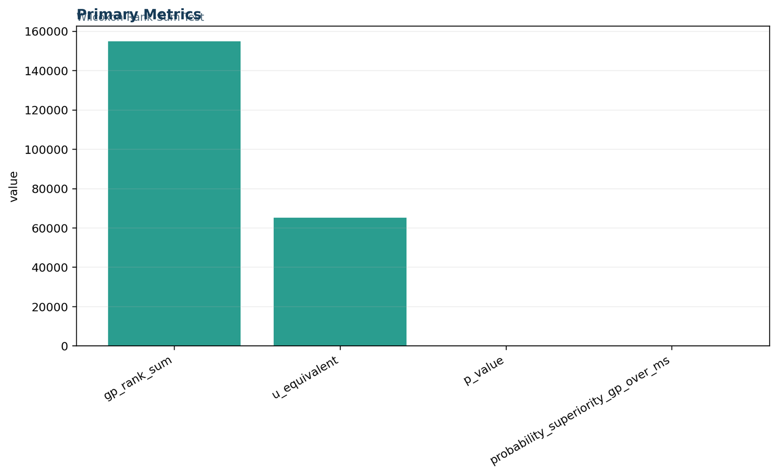
Python chart 1: Primary metrics
The full-width Wilcoxon rank sum test overview displays the GP rank sum of 154,877, the equivalent U statistic of 65,201, the very small two-sided p-value and probability superiority of 0.6820. Because all quantities share one axis, the p-value and probability bar appear near zero relative to the rank totals. Their exact values should be read from the report rather than estimated from bar height.
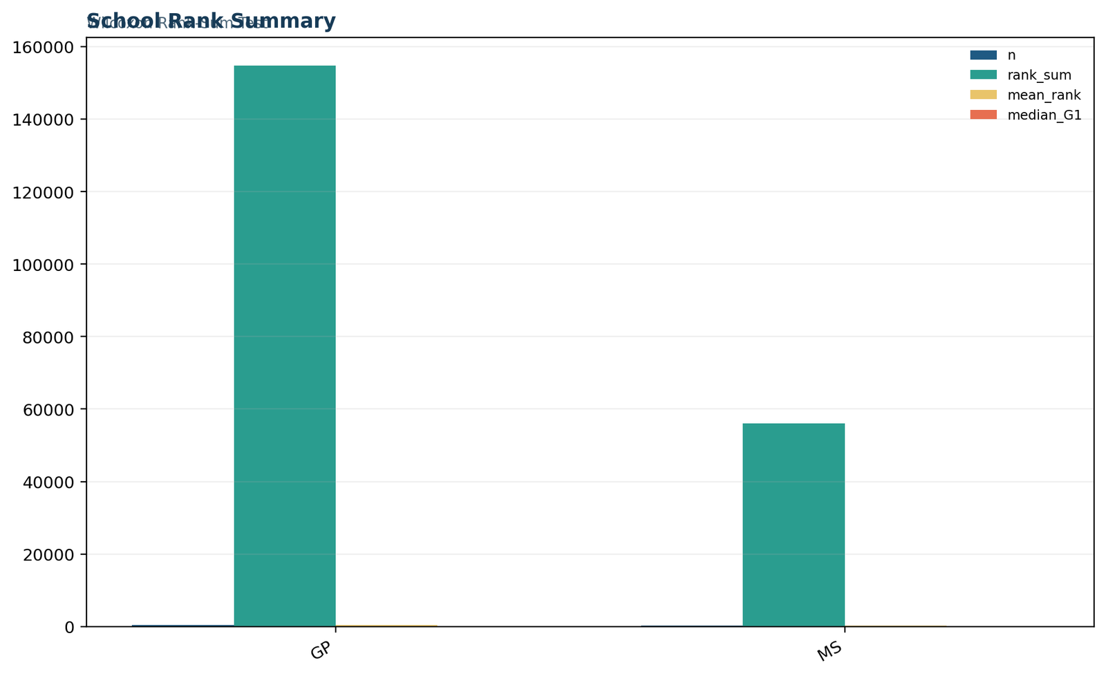
Python chart 2: School rank summary
In the Wilcoxon rank sum test rank table, GP contributes 423 observations, rank sum 154,877, mean rank 366.139 and median G1 = 12. MS contributes 226 observations, rank sum 56,048, mean rank exactly 248 and median G1 = 10. The much higher GP mean rank is the central descriptive signal behind the positive U departure.
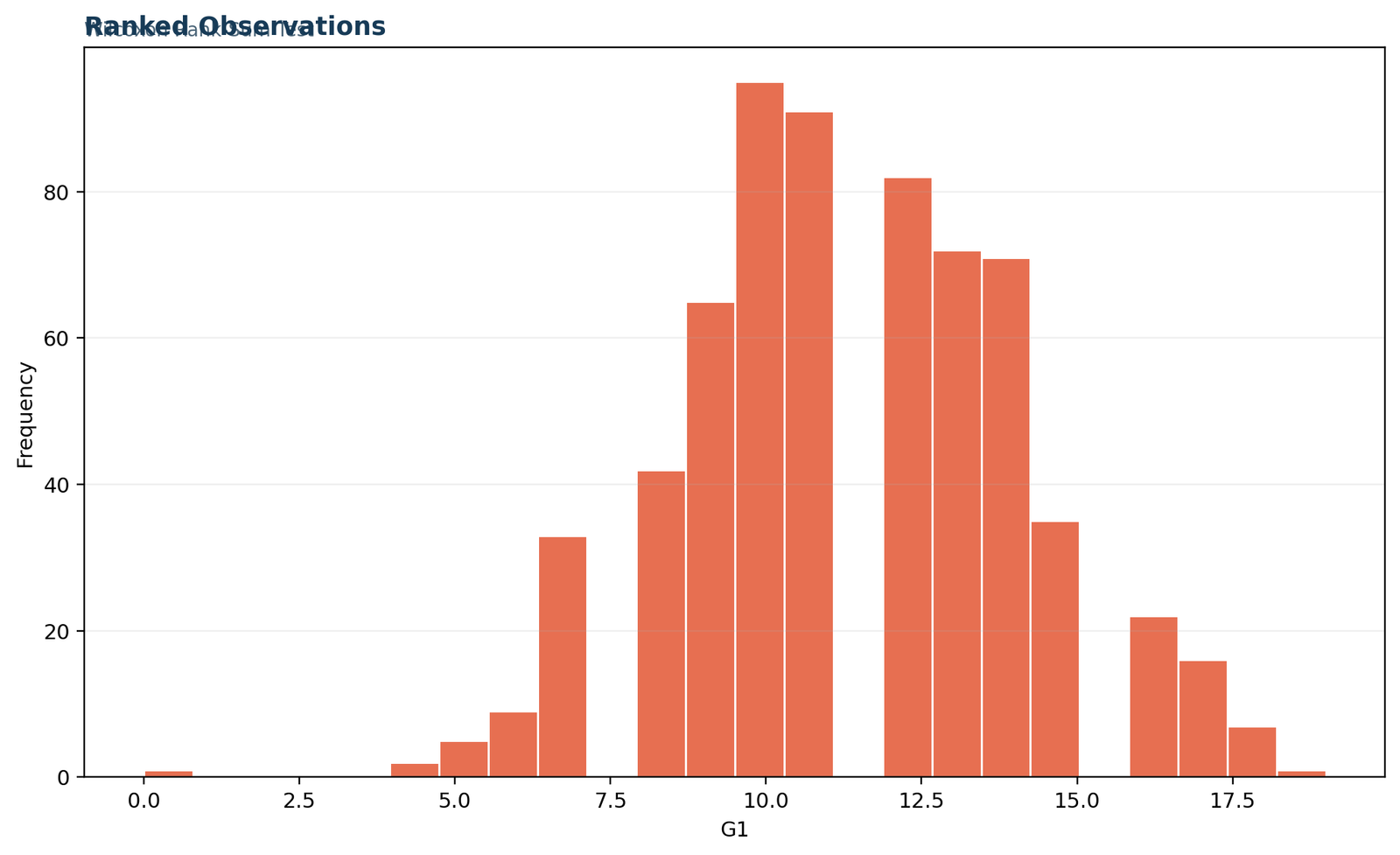
Python chart 3: Ranked observations
The Wilcoxon rank sum test histogram shows the pooled G1 frequency structure from 0 through 19. Integer scores create substantial ties, particularly around 10–14. Those repetitions justify midranks and a tie-adjusted variance. The pooled chart describes overall frequency but should be supplemented by group-specific summaries before attributing the result to a pure location shift.
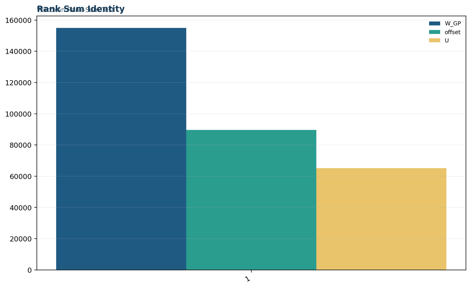
Python chart 4: W-to-U identity
The Wilcoxon rank sum test identity chart decomposes the GP rank sum into the fixed offset and the U equivalent: 154,877 = 89,676 + 65,201. This identity explains why packages can display different-looking statistics while returning the same p-value. The offset depends only on the first-group sample size.
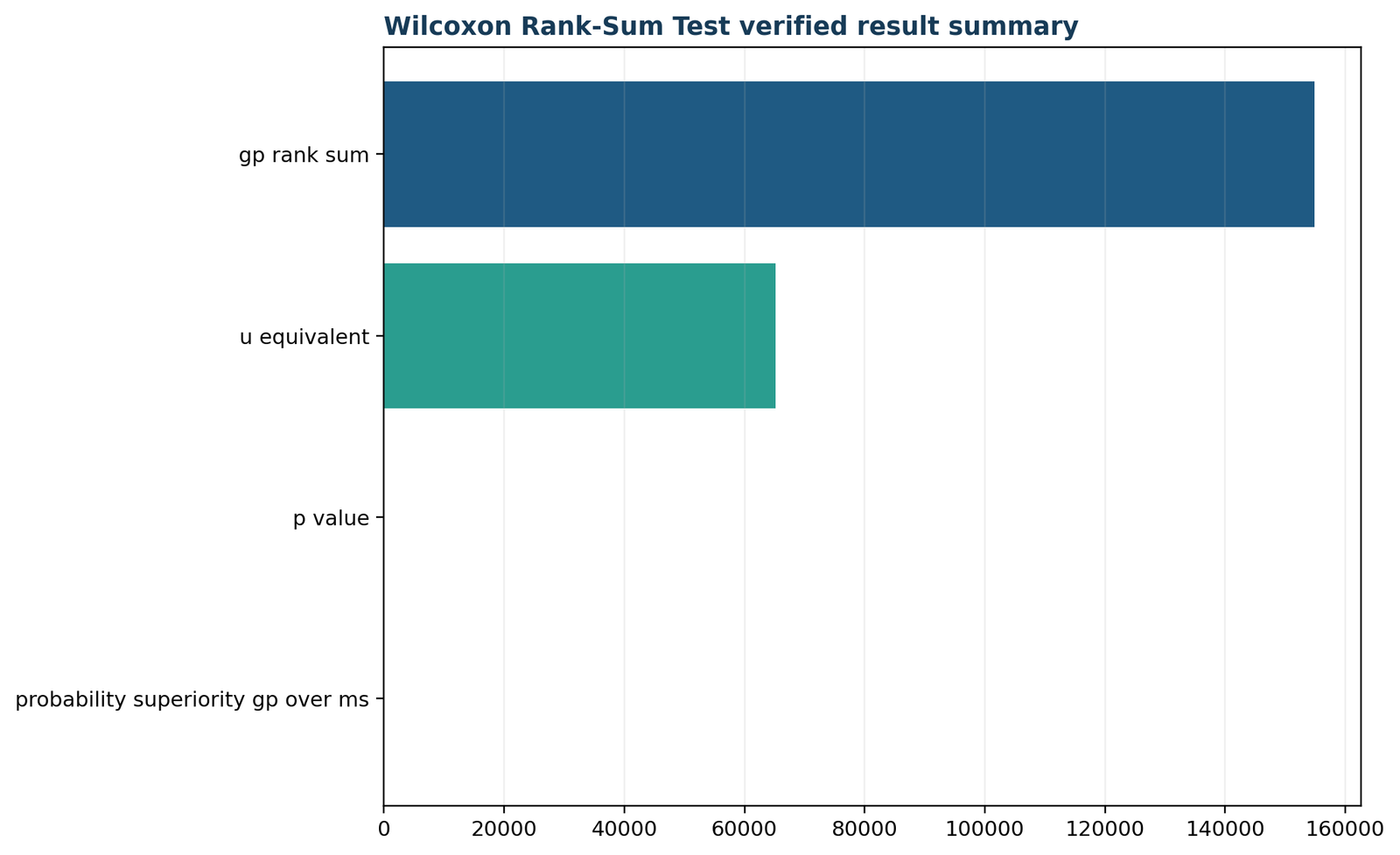
Python chart 5: Verified result summary
The final Wilcoxon rank sum test chart repeats WGP, UGP, the p-value and probability superiority as an audit summary. The statistical conclusion is strongest when the tiny p-value is paired with the 68.20% probability-superiority estimate rather than presented as significance alone.
Wilcoxon rank sum test in R: wilcox.test() and statistic conventions
Base R performs the two-sample Wilcoxon test with continuity correction and optional confidence intervals.
The Wilcoxon rank sum test in R is run with wilcox.test(). With two independent samples and ties, set paired = FALSE, use the normal approximation, and state whether continuity correction was requested.
df <- read.csv("dataset.csv")gp <- df$G1[df$school == "GP"]
ms <- df$G1[df$school == "MS"]
fit <- wilcox.test(
gp, ms,
alternative = "two.sided",
paired = FALSE,
exact = FALSE,
correct = TRUE,
conf.int = TRUE,
conf.level = 0.95
)
fit
What R calls W
For the two-sample procedure, base R’s printed statistic labeled W is commonly the first-sample rank sum after subtracting n1(n1 + 1)/2. With GP supplied first, the printed value is therefore expected to match UGP = 65,201 rather than the raw pooled rank total 154,877.
This naming convention is not an error. Always identify the software and group order when copying the statistic into a report.
Confidence interval meaning
When conf.int = TRUE, R estimates the pseudomedian of pairwise differences under its shift model and provides a confidence interval. This is not automatically a confidence interval for the raw difference between the two sample medians. With many ties, warnings or slight software differences can occur.
n1 <- length(gp)
n2 <- length(ms)U_gp <- unname(fit$statistic)
A_gp <- U_gp / (n1 * n2)
rank_biserial <- 2 * A_gp - 1
c(probability_superiority = A_gp,
rank_biserial = rank_biserial)
R chart 1: Primary metrics
The full-width R Wilcoxon rank sum test overview reproduces the verified rank total, U equivalent, p-value and probability-superiority estimate. The p-value is approximately 1.424 × 10⁻¹⁴, so it is visually compressed by rank totals measured in tens of thousands.
R chart 2: School rank summary
In the R Wilcoxon rank sum test summary, the GP bar for rank sum is larger partly because GP has more observations, so mean rank is the more direct group comparison. Mean rank 366.139 for GP versus 248.000 for MS confirms that GP grades occupy higher pooled positions.
R chart 3: Pooled grade frequencies
The discrete peaks in the Wilcoxon rank sum test chart demonstrate why exact no-tie theory is inappropriate for this dataset. The pooled order contains many tied blocks, and every member of a tied block receives the same average rank.
R chart 4: Statistic identity
For the Wilcoxon rank sum test, the raw rank sum equals the fixed GP offset plus the Mann–Whitney U statistic. This relationship is the key to reconciling R, SciPy, SPSS, MATLAB and textbook output.
R chart 5: Final verification
The closing R Wilcoxon rank sum test summary confirms the same numerical result as the workbook and Python analysis. Agreement across implementations reduces the risk of a group-order, tie-correction or statistic-labeling mistake.
Wilcoxon rank sum test in SPSS: Mann–Whitney U workflow
SPSS labels the equivalent test as Mann–Whitney U in the two-independent-samples procedure.
To run the Wilcoxon rank sum test in SPSS, select the Mann–Whitney U test for two independent samples. SPSS reports a Mann–Whitney statistic, a Wilcoxon rank sum and a standardized value; the displayed raw values can correspond to the smaller group rather than the first group used in Python or Excel.
Legacy dialog steps
Expected statistic reconciliation
If SPSS reports the smaller U, the value is 30,397. Its associated Wilcoxon W is the MS rank sum, 56,048. These are equivalent to the GP-oriented values because UGP + UMS = 95,598 and WGP + WMS = 210,925.
The sign of the standardized z can depend on group coding and rank direction. The p-value and substantive direction should be interpreted using the group-rank table rather than the sign alone.
* Create a numeric group code when school is stored as text.

AUTORECODE VARIABLES=school /INTO school_num.

VALUE LABELS school_num 1 'GP' 2 'MS'.NPAR TESTS

/M-W = G1 BY school_num(1 2)

/STATISTICS = DESCRIPTIVES QUARTILES

/MISSING ANALYSIS.
Wilcoxon rank sum test in Excel: worked formulas with tie correction
Use pooled midranks and formula-driven checks rather than a hand-entered p-value.
The supplied Wilcoxon rank sum test Excel workbook separates raw data, row-level ranks, calculations, diagnostics and reporting. Its structure makes the result auditable from every G1 observation through W, U, the tie term, z and the final p-value.
Recommended workbook logic
| Item | Excel action or formula | Verified result |
|---|---|---|
| Pooled midrank | =RANK.AVG(A5,$A$5:$A$653,1) after pooling all G1 values | One average rank per tied score |
| GP rank sum | =SUMIF($B$5:$B$653,"GP",$C$5:$C$653) | 154,877 |
| GP sample size | =COUNTIF($B$5:$B$653,"GP") | 423 |
| MS sample size | =COUNTIF($B$5:$B$653,"MS") | 226 |
| UGP | =W_GP-n1*(n1+1)/2 | 65,201 |
| Mean U | =n1*n2/2 | 47,799 |
| Tie term | Sum t3 − t across unique G1 values | 3,336,300 |
| Variance U | =n1*n2/12*((N+1)-TieTerm/(N*(N-1))) | 5,115,025.6003 |
| Corrected |z| | =(ABS(U-MeanU)-0.5)/SQRT(VarianceU) | 7.694188 |
| Two-sided p | =2*NORM.S.DIST(-ABS(z),TRUE) | ≈ 1.424E-14 |
How to calculate tie sizes
Create a unique list of G1 values, count each value with COUNTIF, then calculate t^3-t for every count. The total 3,336,300 must be included in the variance. Omitting it produces an incorrect standard error for these highly discrete grades.
How to avoid p = 0
Use the lower-tail formula =2*NORM.S.DIST(-ABS(z),TRUE). The algebraically equivalent expression =2*(1-NORM.S.DIST(ABS(z),TRUE)) can lose precision when the cumulative probability rounds to 1.
Wilcoxon rank sum test in MATLAB, SAS and Stata
Equivalent commands use different labels but test the same independent-sample ordering question.
The Wilcoxon rank sum test is available as ranksum in MATLAB, the Wilcoxon option in SAS PROC NPAR1WAY, and ranksum in Stata. Always verify which group defines the printed rank sum or U statistic.
MATLAB
gp = G1(school == "GP");

ms = G1(school == "MS");[p,h,stats] = ranksum(gp,ms,...

'tail','both',...

'method','approximate');
MATLAB returns the rank sum of the first sample and, for the approximate method, a z value. With GP first, the raw rank sum should be 154,877. Confirm the treatment of ties and continuity correction in the version used.
SAS
proc npar1way data=student wilcoxon;

class school;

var G1;

exact wilcoxon / maxtime=60;

run;
The asymptotic Wilcoxon analysis is appropriate for this large tied dataset. An exact request can be computationally intensive and must use a method that accounts for the observed ties.
Stata
ranksum G1, by(school)

return list
Stata reports rank sums, expected rank sums and a normal approximation. Check the group ordering in the output before interpreting the sign of z.
Wilcoxon rank sum vs Mann–Whitney U, t test and signed rank
Closely related names do not imply identical designs or estimands.
The most common search question is whether the Mann Whitney U test is the same as the Wilcoxon rank sum test. The inferential tests are equivalent for two independent samples; the difference is mainly the raw statistic reported. The Wilcoxon signed rank test, however, is a different paired-sample procedure.
| Method | Design | Main target | Statistic | Important caution |
|---|---|---|---|---|
| Wilcoxon rank sum | Two independent groups | Distributional ordering; location under common shape | Rank sum W | W convention varies by software. |
| Mann–Whitney U | Two independent groups | Same inference as rank sum; pairwise superiority | U | Some software reports U for the first group, others the smaller U. |
| Wilcoxon signed rank | Paired or one-sample differences | Symmetric location of paired differences | Signed-rank sum | Not valid for independent groups. |
| Welch t test | Two independent groups | Difference in population means | t | Targets means and uses metric distances. |
| Brunner–Munzel test | Two independent groups | Relative effect without equal-shape/equal-variance requirement | t-like statistic | Can be preferable when group shapes and variances differ. |
| Two-sample KS test | Two independent groups | Any difference between continuous CDFs | Maximum CDF distance | Different sensitivity and complications with ties. |
| Kruskal–Wallis | Three or more independent groups | Rank-based omnibus difference | H | Requires post-hoc comparisons after significance. |
Wilcoxon rank sum vs t test
The rank test is not simply a t test without normality. Welch’s t test targets the mean difference and uses the magnitude of each observation. The rank test targets ordering and is less sensitive to extreme numeric distances. Under normal location shifts, the t test is usually more efficient; under heavy tails or influential outliers, the rank approach can be more stable.
Wilcoxon rank sum vs median test
The median test reduces each observation to above/below a pooled median and discards much rank information. It can be useful for a narrowly defined median question but usually has lower power than the full rank-sum procedure. The rank-sum result should still not be called a median test unless shape conditions are satisfied.
Diagnostics, sensitivity checks, sample size and power
Inspect design and distributions before relying on the final p-value.
A strong Wilcoxon rank sum test analysis includes group-size checks, missing-value handling, pooled ties, distribution-shape diagnostics, alternative-statistic conventions, effect size and a power discussion. The method is robust to many non-normal shapes but not to dependence or an undefined estimand.
Independence audit
Check whether students are nested in classrooms or families, whether repeated records exist and whether school membership was sampled independently. A large nominal N cannot compensate for pseudoreplication.
Missing-data audit
Confirm that the same 649 complete records appear in all software. Report the rule for missing G1 or school values. A different valid-case set changes ranks for every included observation.
Tie audit
List the frequency of each observed grade and verify midranks. For small samples with ties, prefer a permutation procedure that conditions on the observed pooled values rather than a no-tie exact distribution.
Shape audit
Compare ECDFs, histograms, boxplots and quantiles. Similar IQRs of 4 support a location comparison, but the different SDs and ranges show that shape equality should not be asserted without visual evidence.
Direction audit
Confirm which group was entered first. A positive GP-oriented U departure indicates higher GP ranks, while software that reports the smaller U can attach a negative z to the same substantive result.
Effect-size audit
Report probability superiority or rank-biserial correlation. Avoid presenting z/√N as the only magnitude estimate because it depends on total sample size and does not translate as directly into pairwise ordering.
Power and sample-size planning
Power depends on the full alternative distribution, not only on a median difference. Simulation is often the clearest planning approach: specify plausible GP and MS distributions, sample repeatedly at candidate sizes, run the same tie-aware procedure and estimate the proportion of rejected null hypotheses.
For a probability-superiority target, planning can also be framed around the expected A parameter. The observed A = .682 is large enough that the present samples have overwhelming evidence, but a future study should use a conservative effect grounded in substantive importance rather than reusing the observed estimate without shrinkage.
Sensitivity analysis for this example
The no-correction and continuity-corrected p-values are nearly identical. The median difference and Hodges–Lehmann shift are both two points. Probability superiority, rank-biserial correlation and mean ranks all point in the same direction. This convergence makes the conclusion more stable than a decision based on one p-value alone.
A Welch t test could answer the separate mean-difference question, while Brunner–Munzel could test relative effect with weaker equal-shape requirements. Agreement across these conceptually different analyses would strengthen the descriptive conclusion, but each result must retain its own estimand.
How to report the Wilcoxon rank sum test in APA style
Include group summaries, statistic convention, p-value method, direction and effect size.
An APA-style Wilcoxon rank sum test report should identify the independent groups and outcome, explain whether W or U is reported, provide the continuity-corrected z and p-value, describe medians or rank summaries, and include a practical effect measure.
Recommended narrative
When the journal or software convention expects the smaller U, the same analysis can be reported as U = 30,397. State the group order or software source so readers can reconcile the number. Do not report both 65,201 and 30,397 without explaining that they are complementary statistics.
Minimum reporting checklist
Interpretive language to avoid
Avoid “the Wilcoxon test proves GP causes higher grades,” “the means are significantly different,” “the medians are unequal” without a shape qualification, and “p = 0.000.” Prefer “GP observations tended to be higher,” “the distributions differed,” and “under a common-shape interpretation, GP had the higher location.”
Wilcoxon rank sum test PDF, Excel and software downloads
Use the complete outputs to reproduce and audit the worked analysis.
Download the Wilcoxon rank sum test reports for Python, R and SPSS, plus the formula-driven Excel workbook containing raw data, pooled ranks, calculations, diagnostics and reporting checks.
Python report PDFVerified SciPy calculation, descriptive results and charts.Download PDF →
R report PDFR workflow, statistics and reproducible output.Download PDF →
SPSS output PDFMann–Whitney U output and group-rank tables.Download PDF →
Worked Excel analysisRaw input, midranks, tie correction, formulas and audit checks.Download workbook →
Official Wilcoxon rank sum references and software documentation
Method identity and implementation details were checked against primary documentation.
Reliable Wilcoxon rank sum test guidance should distinguish the broad equal-distributions null, the common-shape location interpretation, the W-to-U identity, exact versus asymptotic inference, ties and software-specific statistic conventions.
mannwhitneyu documentation. Documents the first-sample U statistic, W-to-U conversion, independent-sample design, exact/asymptotic/permutation methods and treatment of ties.stats::wilcox.test documentation. Documents the two-sample test, continuity correction, exact option, one-sided alternatives and shift confidence interval.ranksum documentation. Provides the rank-sum statistic, U identity, tie-adjusted normal approximation, continuity correction and exact/approximate method rules.Wilcoxon rank sum test FAQs
Clear answers to the most common formula, assumption, software and interpretation questions.
What is a Wilcoxon rank sum test?
The Wilcoxon rank sum test is a nonparametric test for comparing two independent samples. It pools the observations, assigns ranks and tests whether one group tends to occupy higher ranks than the other.
Is the Mann–Whitney U test the same as the Wilcoxon rank sum test?
The Wilcoxon rank sum test and Mann–Whitney U procedures are inferentially equivalent. The Wilcoxon form emphasizes a rank sum W; the Mann–Whitney form emphasizes a pair-count statistic U. Software can report either orientation.
Is the Wilcoxon signed rank test the same test?
The Wilcoxon rank sum test is not the signed-rank test. Signed rank is for paired observations or one-sample differences. Rank sum is for two independent groups.
What does the Wilcoxon rank sum test measure?
The Wilcoxon rank sum test measures whether one population tends to generate higher observations than the other. Broadly it tests equality of distributions; under common shape it can be interpreted as a location or median-shift test.
What are the main assumptions?
For the Wilcoxon rank sum test, the samples and observations should be independent, the outcome must be orderable, the sampling design must justify inference, ties must be handled correctly, and similar shapes are needed for a pure median interpretation.
Can the sample sizes be unequal?
The Wilcoxon rank sum test permits unequal sample sizes. The worked example uses 423 GP observations and 226 MS observations. Unequal sizes are included directly in the W, U, expectation and variance formulas.
How are tied values ranked?
In the Wilcoxon rank sum test, every observation in a tie block receives the average of the ranks occupied by that block. The normal-approximation variance must also be reduced using the tie term.
What is W in the Wilcoxon rank sum test?
In the textbook Wilcoxon rank sum test form, W is the pooled rank total for a selected group. Some software uses W for an offset statistic equivalent to U, so the convention must be stated.
How are W and U related?
For the Wilcoxon rank sum test, group 1 has U = W − n₁(n₁ + 1)/2. In the example, 154,877 − 89,676 = 65,201.
What was the worked-example result?
The worked Wilcoxon rank sum test gave GP W = 154,877 and U = 65,201, with continuity-corrected z = 7.694 and two-sided p approximately 1.424 × 10⁻¹⁴.
How should the p-value be interpreted?
For the Wilcoxon rank sum test, under the equal-distributions null, a rank separation at least as extreme as the observed result is extraordinarily unlikely. The p-value does not measure the probability that the null is true or the size of the effect.
What is probability superiority?
For the Wilcoxon rank sum test, probability superiority is U/(n₁n₂). In this analysis it is .682, meaning a random GP grade is higher than a random MS grade, ties counted one-half, 68.2% of the time.
What effect size should be reported?
For a Wilcoxon rank sum test, probability superiority and rank-biserial correlation are direct choices. The analysis reports A = .682 and rrb = .364. A Hodges–Lehmann shift can also be useful under a location model.
Does a significant result prove the medians differ?
A significant Wilcoxon rank sum test does not prove a median difference in every situation. The test can respond to differences in spread or shape. A median-shift conclusion requires reasonably similar distribution shapes.
How do I run the test in Python?
Run the Wilcoxon rank sum test in Python with scipy.stats.mannwhitneyu with the two independent arrays, the planned alternative and an appropriate exact, asymptotic or permutation method.
How do I run the test in R?
Run the Wilcoxon rank sum test in R with wilcox.test(x, y, paired = FALSE) or the formula interface. With ties and large samples, use the asymptotic method and state the continuity-correction choice.
How do I run the test in SPSS?
Run the Wilcoxon rank sum test in SPSS by choosing the Mann–Whitney U option under two independent samples, define the two group codes, and inspect the rank table, U, Wilcoxon W, z and significance.
How do I calculate it in Excel?
Calculate the Wilcoxon rank sum test in Excel by pooling the observations, assigning RANK.AVG midranks, sum one group’s ranks, convert W to U, calculate the tie-adjusted variance, continuity-correct z and use the standard normal lower tail for the p-value.
Related statistical guides
Continue with methods that clarify independent samples, paired samples, distribution shape and effect size.