
ANOVA Post Hoc Test, Unequal Group Sizes, Harmonic Mean Sample Size
Hochbergs GT2: Formula, Interpretation, SPSS, Python, R and Excel Guide
Hochbergs GT2, usually written as Hochberg’s GT2, is a post hoc multiple comparison method used after one-way ANOVA to compare group means pair by pair. It is commonly used when equal variances are assumed and group sizes are unequal. This guide explains Hochbergs GT2 with SPSS output, Python charts, R validation, Excel workflow, harmonic mean sample size, pairwise p-values, confidence intervals, APA reporting and downloadable resources.
Quick Answer: Hochbergs GT2 Result
The worked example compares G3 final grade across four studytime groups. The sample contains 649 students. The omnibus one-way ANOVA was statistically significant, F(3, 645) = 15.876, p < .001, so post hoc pairwise comparisons were justified. Hochbergs GT2 was then used to identify which studytime groups differed from each other.
The group means increased from the lowest studytime group to the higher studytime groups. Group 1 had the lowest mean G3 score, M = 10.84. Group 2 had M = 12.09. Group 4 had M = 13.06. Group 3 had the highest mean, M = 13.23. Hochbergs GT2 found 4 significant pairwise comparisons out of 6 total comparisons.
Final interpretation: Hochbergs GT2 shows that studytime group 1 differs significantly from groups 2, 3 and 4. Group 2 also differs significantly from group 3. The comparisons 2 vs 4 and 3 vs 4 are not statistically significant. In plain language, students in the lowest studytime category had lower final grades than students in the higher studytime categories, while the highest studytime groups were not clearly different from each other.
Important reporting point: SPSS uses a harmonic mean sample size for Hochberg’s GT2 when group sizes are unequal. In this example, the harmonic mean sample size is approximately 85.331. SPSS also warns that Type I error levels are not guaranteed when group sizes are unequal, so the result should be interpreted as a post hoc comparison under unequal sample-size conditions.
Table of Contents
- What Is Hochbergs GT2?
- When to Use Hochbergs GT2
- Hochbergs GT2 Formula and Decision Logic
- Null and Alternative Hypotheses
- Dataset and Variables Used
- SPSS Output Interpretation
- Python Chart-by-Chart Interpretation
- R Chart-by-Chart Validation
- SPSS, R, Python and Excel Workflows
- Code Blocks for Hochbergs GT2
- APA Reporting Wording
- Common Mistakes
- Downloads and Resources
- Related Guides
- FAQs
What Is Hochbergs GT2?
Hochbergs GT2 is a post hoc multiple comparison test used after a one-way ANOVA. It compares all possible pairs of group means and adjusts the decision for the fact that several pairwise comparisons are being made. In SPSS, it appears as Hochberg’s GT2 in the post hoc test options.
The purpose of Hochbergs GT2 is to answer the question that ANOVA does not answer by itself. ANOVA tells whether at least one group mean differs, but it does not identify exactly which groups are different. Hochbergs GT2 compares each group pair and reports the mean difference, standard error, significance value and confidence interval.
Hochbergs GT2 is often discussed for designs with unequal group sizes under the equal-variance ANOVA framework. It uses the harmonic mean sample size when group sizes are unequal. That is why the group-size structure must be reported clearly when interpreting this test.
Simple definition: Hochbergs GT2 is an ANOVA post hoc test for comparing group means pair by pair, especially when group sizes are unequal but equal variances are assumed.
Before using Hochbergs GT2, review one-way ANOVA, ANOVA assumptions, Levene test, p-values, confidence intervals, and effect size.
When to Use Hochbergs GT2
Use Hochbergs GT2 when you have a one-way ANOVA with three or more groups, a continuous dependent variable, an overall significant ANOVA result, and a need to compare all pairs of group means. It is especially relevant when group sizes are unequal but the equal-variance assumption is acceptable.
| Use Hochbergs GT2 When | Why It Matters | Example in This Guide |
|---|---|---|
| The omnibus ANOVA is significant | Post hoc testing is justified after evidence that at least one group mean differs. | ANOVA p < .001. |
| You need pairwise comparisons | ANOVA does not identify which specific group pairs differ. | Four studytime groups create six pairwise comparisons. |
| Group sizes are unequal | Hochberg’s GT2 uses the harmonic mean sample size in unequal-size designs. | Group sizes are 212, 305, 97 and 35. |
| Equal variances are acceptable | Hochberg’s GT2 belongs to the equal-variance ANOVA post hoc family. | Levene test based on mean was not significant, p = .400. |
When not to use it: If variances are clearly unequal, a method such as Games-Howell may be safer. If group sizes are extremely unequal, interpret Hochbergs GT2 carefully because SPSS warns that Type I error levels are not guaranteed when unequal group sizes are handled through the harmonic mean sample size.
Hochbergs GT2 Formula and Decision Logic
Hochbergs GT2 compares group means using the pooled ANOVA error term and a multiple-comparison critical value. The basic pairwise mean difference is:
The pooled within-group mean square error comes from the ANOVA table:
For pairwise comparison, the standard error is based on the ANOVA MSE and the group sample sizes:
When group sizes are unequal, SPSS reports that the harmonic mean sample size is used. A simplified harmonic mean idea is:
The pairwise decision is then based on whether the adjusted p-value is below α = .05 or whether the confidence interval excludes zero.
| Symbol | Meaning | Interpretation |
|---|---|---|
| Mi, Mj | Group means | The two studytime group means being compared. |
| MSE | Mean square error | The pooled within-group error estimate from ANOVA. |
| ni, nj | Group sample sizes | The sample sizes for the compared pair. |
| nh | Harmonic mean sample size | Used by SPSS when group sizes are unequal. |
| Adjusted p-value | Post hoc significance value | Used to decide whether a pairwise difference is significant. |
Decision rule: A pair is significant when the adjusted p-value is below .05 or when the Hochberg GT2 confidence interval for the mean difference excludes zero.
Null and Alternative Hypotheses for Hochbergs GT2
Hochbergs GT2 is interpreted pair by pair. Each comparison has its own null and alternative hypothesis. The null says the two population means are equal. The alternative says the two population means are different.
| Pairwise Test | Hypothesis | Meaning |
|---|---|---|
| Null hypothesis | H0: μi = μj | The two studytime groups have equal mean G3 scores. |
| Alternative hypothesis | H1: μi ≠ μj | The two studytime groups have different mean G3 scores. |
| Decision rule | Adjusted p < .05 or CI excludes 0 | The pair is significant by Hochbergs GT2. |
Decision for this example: The significant comparisons are 1 vs 2, 1 vs 3, 1 vs 4, and 2 vs 3. The non-significant comparisons are 2 vs 4 and 3 vs 4.
Dataset and Variables Used
The worked example uses a student performance dataset. The dependent variable is G3 final grade. The factor is studytime, coded into four weekly study-time categories. The analysis asks whether average final grade differs across studytime groups and which pairs of groups are significantly different after the ANOVA.
| Variable | Role | How It Is Used in Hochbergs GT2 |
|---|---|---|
| G3 | Dependent variable | The final grade score being compared across studytime groups. |
| studytime | Grouping factor | The four-level factor used in one-way ANOVA and Hochberg GT2 post hoc comparisons. |
| Group 1 | < 2 hours | Lowest studytime group and lowest mean G3 score. |
| Group 2 | 2 to 5 hours | Middle studytime group with a higher mean than group 1. |
| Group 3 | 5 to 10 hours | Highest mean G3 score in this example. |
| Group 4 | > 10 hours | High mean G3 score but not significantly different from groups 2 or 3. |
Before interpreting Hochbergs GT2, review the group distributions, means, sample sizes and variance context. Helpful related guides include descriptive statistics, box plot interpretation, Levene test, and ANOVA in SPSS.
SPSS Output Interpretation for Hochbergs GT2
The SPSS output provides the official Hochberg’s GT2 post hoc table. It begins with group descriptives, checks homogeneity of variances, reports the one-way ANOVA and then lists the Hochberg multiple comparisons and homogeneous subsets.
SPSS Group Descriptives
| Studytime Group | N | Mean G3 | Std. Deviation | Variance | Minimum | Maximum | Interpretation |
|---|---|---|---|---|---|---|---|
| 1 | 212 | 10.84 | 3.219 | 10.360 | 0 | 18 | Lowest average final grade. |
| 2 | 305 | 12.09 | 3.243 | 10.518 | 0 | 19 | Higher than group 1. |
| 3 | 97 | 13.23 | 2.502 | 6.261 | 8 | 18 | Highest average final grade. |
| 4 | 35 | 13.06 | 3.038 | 9.232 | 6 | 19 | Similar to group 3 but with a smaller sample size. |
| Total | 649 | 11.91 | 3.231 | 10.437 | 0 | 19 | Overall final grade mean. |
SPSS Homogeneity of Variances
| Test | Statistic | df1 | df2 | p-value | Interpretation |
|---|---|---|---|---|---|
| Levene test based on mean | 0.985 | 3 | 645 | .400 | Not significant; the equal-variance assumption is acceptable for this example. |
| Levene test based on median | 1.026 | 3 | 645 | .380 | Also not significant; supports the same variance conclusion. |
| Levene test based on trimmed mean | 1.081 | 3 | 645 | .356 | No strong variance warning from the trimmed mean version. |
SPSS One-Way ANOVA Table
| Source | Sum of Squares | df | Mean Square | F | Sig. | Interpretation |
|---|---|---|---|---|---|---|
| Between Groups | 465.078 | 3 | 155.026 | 15.876 | < .001 | At least one studytime group mean differs. |
| Within Groups | 6298.189 | 645 | 9.765 | Pooled error term used in equal-variance post hoc comparisons. | ||
| Total | 6763.267 | 648 | Total variation in G3. |
SPSS Hochberg GT2 Multiple Comparisons
| Comparison | Mean Difference | Std. Error | SPSS Sig. | 95% CI | Hochberg GT2 Decision | Plain Interpretation |
|---|---|---|---|---|---|---|
| 1 vs 2 | -1.247 | .279 | < .001 | [-1.98, -0.51] | Significant | Group 1 scored significantly lower than group 2. |
| 1 vs 3 | -2.382 | .383 | < .001 | [-3.39, -1.37] | Significant | Group 1 scored significantly lower than group 3. |
| 1 vs 4 | -2.213 | .570 | .001 | [-3.72, -0.71] | Significant | Group 1 scored significantly lower than group 4. |
| 2 vs 3 | -1.135 | .364 | .011 | [-2.10, -0.17] | Significant | Group 2 scored significantly lower than group 3. |
| 2 vs 4 | -0.965 | .558 | .408 | [-2.44, 0.51] | Not significant | Groups 2 and 4 do not differ clearly at α = .05. |
| 3 vs 4 | 0.170 | .616 | 1.000 | [-1.46, 1.80] | Not significant | Groups 3 and 4 are statistically similar in this analysis. |
SPSS Homogeneous Subsets
The SPSS homogeneous subsets table shows a lower subset containing group 1 and a higher subset containing groups 2, 4 and 3. Group 2 appears in the transition pattern because it is between the lowest group and the highest groups. This supports the post hoc table: group 1 is the main low-performing group, while the higher studytime groups are not all clearly separated from each other.
SPSS interpretation summary: The one-way ANOVA is significant, Levene’s test does not show a strong variance problem, and Hochberg’s GT2 identifies four significant pairwise differences. The strongest contrast is between studytime group 1 and group 3. The comparison between groups 3 and 4 is clearly not significant.
Python Chart-by-Chart Interpretation
The Python charts show the Hochbergs GT2 workflow visually. They include group distributions, group means, sample-size and variance context, pairwise p-values, mean-difference intervals, a p-value heatmap and significant difference counts.
Python Chart 1: Group Distribution Boxplots
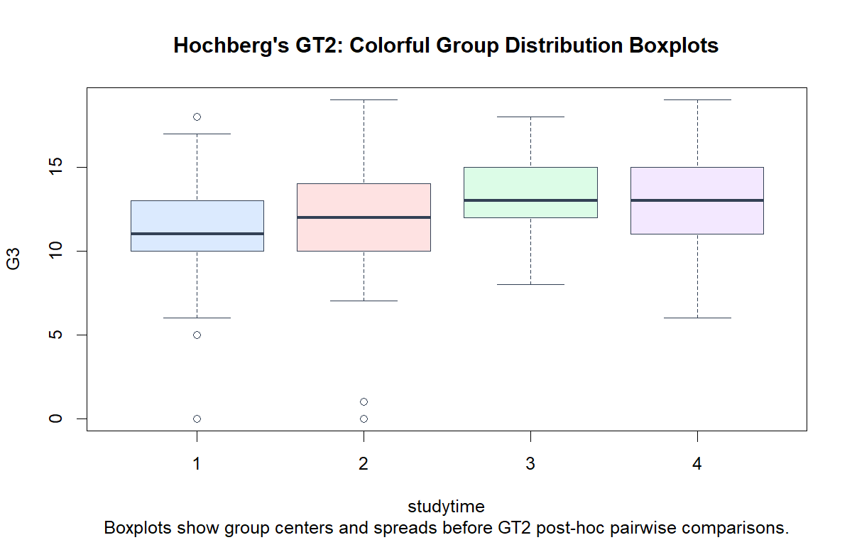
The group distribution chart shows that group 1 has the lowest central position, while groups 3 and 4 are centered higher. Group 2 sits between the lowest and highest studytime categories. This visual pattern explains why the overall ANOVA is significant and why post hoc comparisons are needed.
The boxplots also show that the lower studytime groups include more very low G3 values. Hochbergs GT2 compares means, so the boxplots should be read as context rather than as the final decision table.
Python Chart 2: Group Means with Confidence Intervals
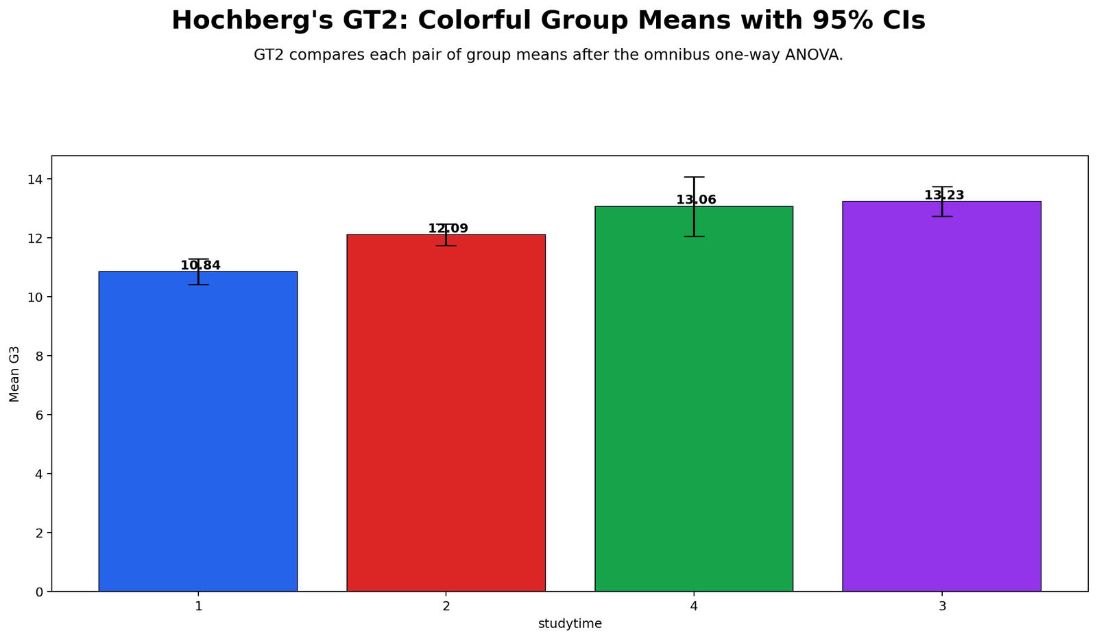
The group means chart shows the same mean order as the SPSS table. Group 1 has the lowest mean, group 2 is higher, and groups 4 and 3 are the highest. The chart makes the practical direction of the result easy to see before reading the detailed post hoc table.
The largest mean gap is between group 1 and group 3. The smallest gap is between groups 3 and 4. This is why group 1 appears in several significant comparisons while group 3 and group 4 do not significantly differ.
Python Chart 3: Group Size and Variance Context
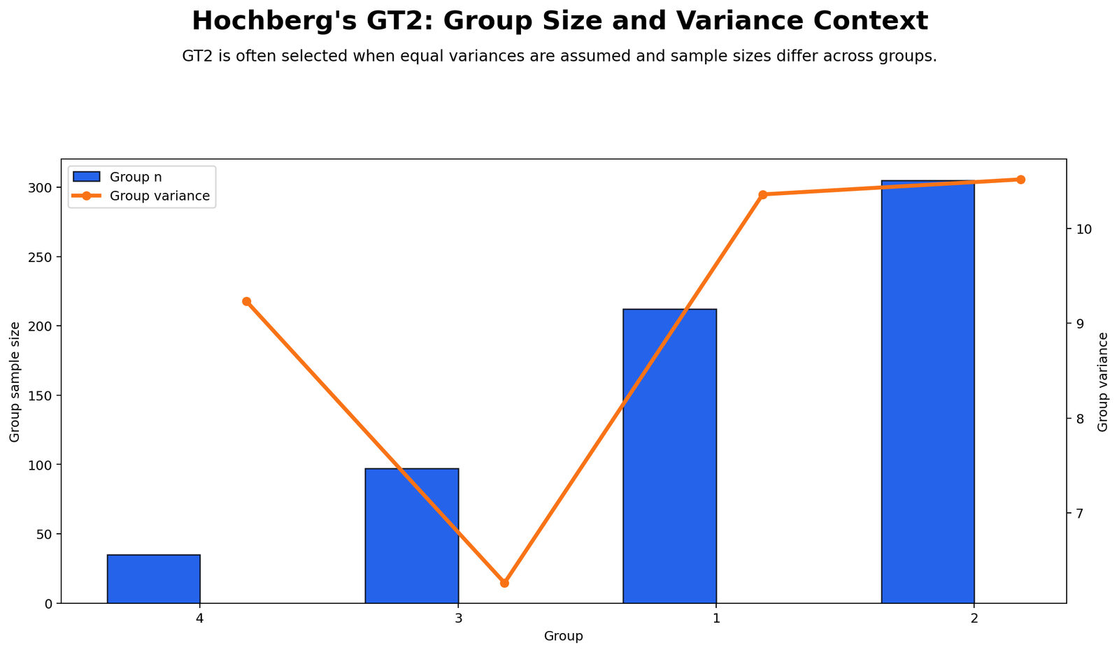
The group size and variance context chart explains why Hochbergs GT2 is relevant. The studytime groups are unequal in size: group 2 is the largest group, group 1 is also large, group 3 is smaller and group 4 is the smallest. Hochberg’s GT2 handles unequal group sizes through the harmonic mean sample size.
The variance pattern also helps interpret the post hoc method. Although the Levene test is not significant, the group variances are not identical. Reporting the variance context makes the post hoc decision more transparent.
Python Chart 4: Hochbergs GT2 Pairwise p-values
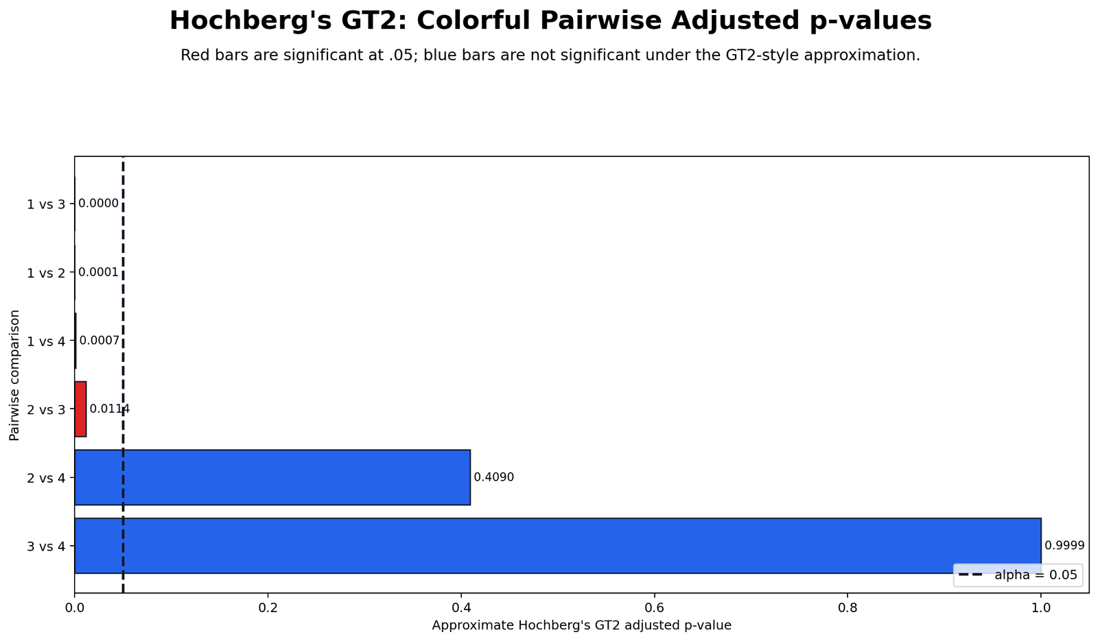
The pairwise p-value chart shows which comparisons are below α = .05. The significant comparisons are 1 vs 3, 1 vs 2, 1 vs 4, and 2 vs 3. These are the pairs where the mean difference is large enough after the Hochberg GT2 adjustment.
The non-significant comparisons are 2 vs 4 and 3 vs 4. The group 3 vs group 4 comparison has a very large p-value, which supports the conclusion that these two higher studytime groups are statistically similar.
Python Chart 5: Hochbergs GT2 Mean Difference Confidence Intervals
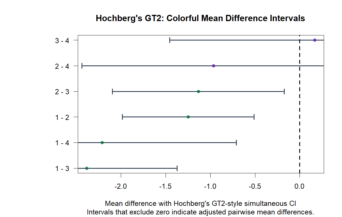
The mean difference chart uses zero as the no-difference line. Intervals that do not cross zero are significant. The intervals for 1 vs 2, 1 vs 3, 1 vs 4, and 2 vs 3 exclude zero.
The intervals for 2 vs 4 and 3 vs 4 cross zero. That means those observed mean differences are not statistically clear after the Hochberg GT2 adjustment. This chart gives a visual explanation of the confidence-interval decision rule.
Python Chart 6: Hochbergs GT2 p-value Heatmap
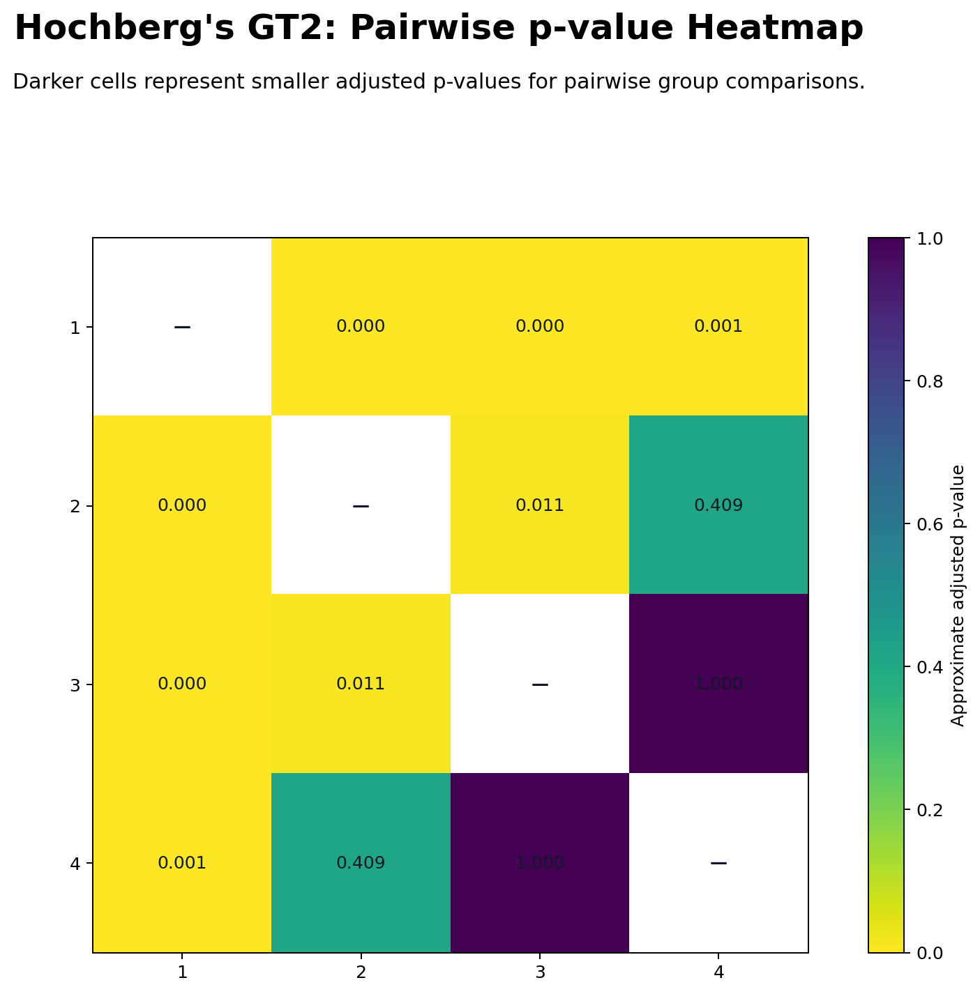
The p-value heatmap gives a compact matrix view of the same pairwise decisions. It shows that group 1 differs from each higher group and that group 2 differs from group 3. These cells represent the main significant post hoc findings.
The heatmap also makes the non-significant pairs easy to see. Groups 2 and 4 do not differ clearly, and groups 3 and 4 are very close. This supports a careful interpretation rather than claiming that every studytime group differs from every other group.
Python Chart 7: Significant Difference Count by Group
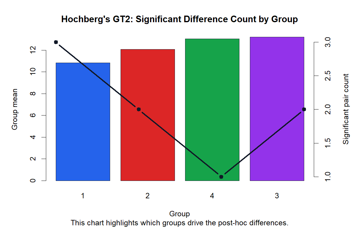
The significant difference count chart shows which groups drive the post hoc result. Group 1 is involved in three significant differences because it differs from groups 2, 3 and 4. Group 2 is involved in two significant differences because it differs from group 1 and group 3.
Group 4 is significantly different from group 1 only, while group 3 is high in mean G3 but not significantly different from group 4. This chart turns the post hoc table into a practical group-level summary.
R Chart-by-Chart Validation
The R validation charts confirm the same substantive result. The same group mean order appears, the same significant comparisons are identified, and the same non-significant comparisons remain non-significant.
R Chart 1: Group Distribution Boxplots
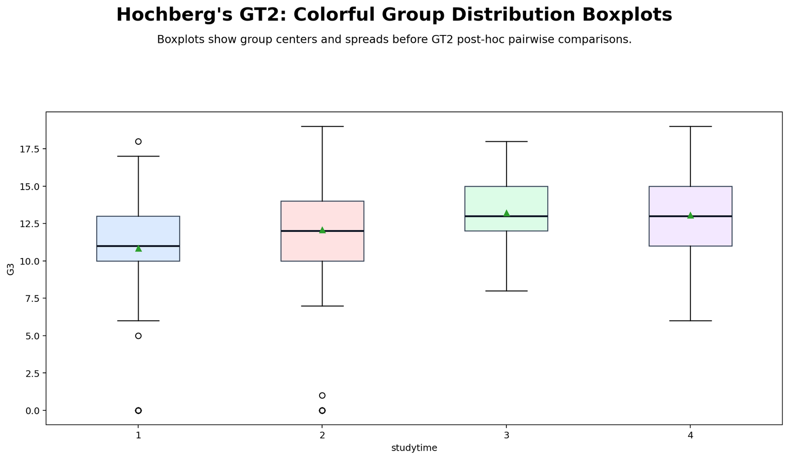
The R boxplot confirms the same distribution pattern shown by Python and SPSS. Group 1 has the lowest central position, group 2 is higher, and groups 3 and 4 are centered near the top.
This agreement across software strengthens the interpretation. The post hoc differences are not caused by one plotting method; they reflect the actual group mean structure.
R Chart 2: Group Means with Confidence Intervals
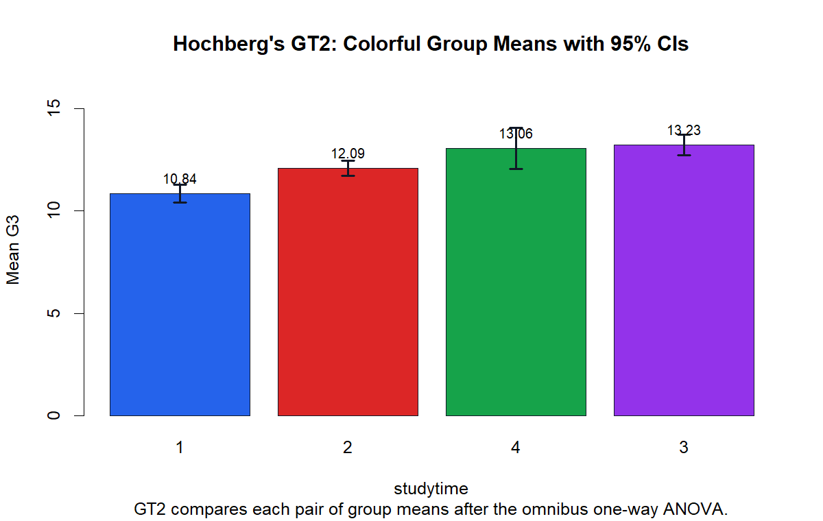
The R group means chart validates the Python mean pattern. Group 1 has the lowest mean, group 3 has the highest mean and group 4 is close to group 3.
This chart explains why groups 3 and 4 are not significantly different. Their mean gap is small compared with the uncertainty around the estimates.
R Chart 3: Group Size and Variance Context
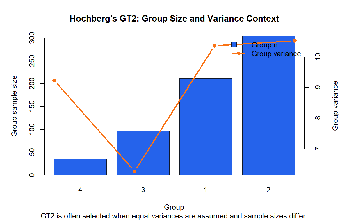
The R group-size and variance chart confirms the unequal group-size structure. Group 4 is much smaller than groups 1 and 2, which is why the harmonic mean sample size note matters for Hochberg’s GT2.
The variance context is also useful because Hochberg’s GT2 is used under an equal-variance ANOVA framework. Reporting this chart helps readers see the assumption context before the post hoc decisions.
R Chart 4: Hochbergs GT2 Pairwise p-values
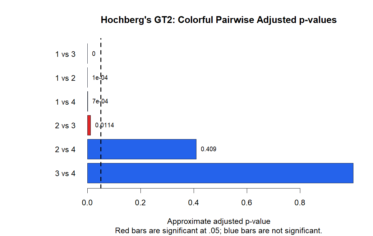
The R p-value chart confirms the same four significant pairs: 1 vs 2, 1 vs 3, 1 vs 4, and 2 vs 3. These p-values are below the .05 threshold.
The non-significant pairs remain 2 vs 4 and 3 vs 4. This software-to-software agreement supports the final interpretation.
R Chart 5: Hochbergs GT2 Mean Difference Confidence Intervals
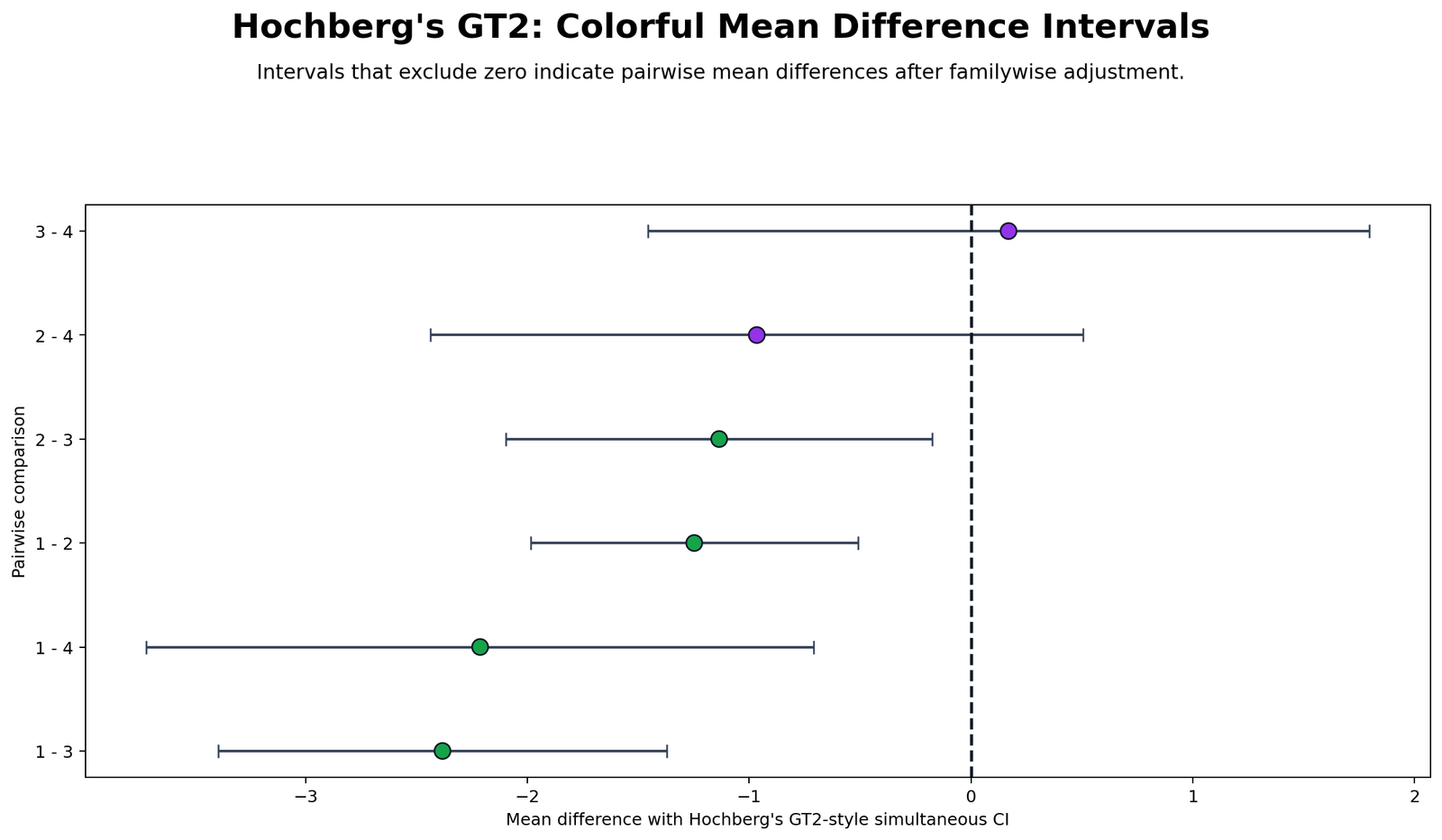
The R confidence interval chart validates the same interval decisions. Significant pairs have intervals that stay away from zero, while non-significant pairs cross zero.
The strongest difference is group 1 compared with group 3. The smallest difference is group 3 compared with group 4. This matches the SPSS post hoc table and the Python confidence interval chart.
R Chart 6: Hochbergs GT2 p-value Heatmap
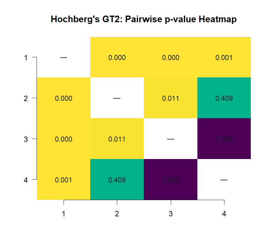
The R heatmap summarizes the pairwise decisions in a compact matrix. It shows that group 1 is the main separated group because it differs from all higher studytime groups.
The heatmap also shows that groups 3 and 4 are not meaningfully separated by the post hoc test. This prevents the common reporting mistake of claiming all higher studytime levels are different from one another.
R Chart 7: Significant Difference Count by Group
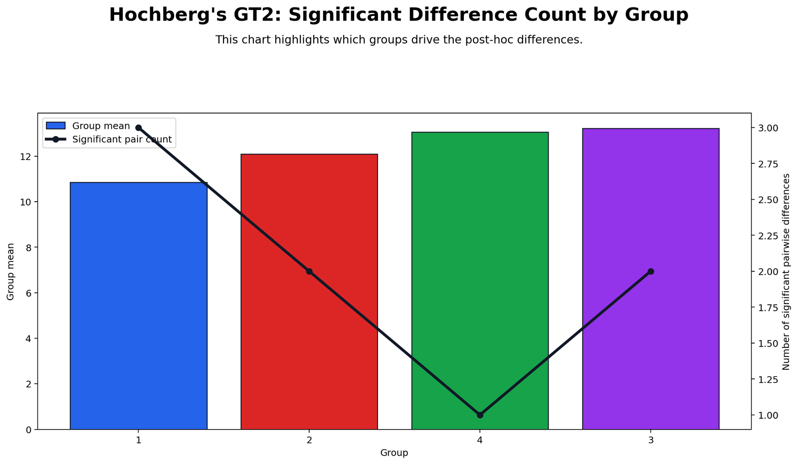
The R significant difference count chart confirms that group 1 drives the result. Group 1 differs from groups 2, 3 and 4, making it the clearest low-performing category.
The higher studytime groups show fewer significant differences among themselves. The final conclusion should therefore emphasize lower performance in group 1 rather than claiming a complete step-by-step difference across every group.
SPSS, R, Python and Excel Workflows for Hochbergs GT2
The same Hochbergs GT2 workflow can be reproduced in SPSS, R, Python and Excel. SPSS gives the easiest official Hochberg GT2 menu output. Python and R are useful for reproducible analysis and custom charts. Excel is useful for understanding the underlying pairwise comparison logic, although it does not provide a one-click Hochberg GT2 post hoc menu.
SPSS Workflow
| Step | SPSS Action | Purpose |
|---|---|---|
| Open data | File > Open > Data | Load the cleaned dataset containing G3 and studytime. |
| Run one-way ANOVA | Analyze > Compare Means > One-Way ANOVA | Set G3 as dependent variable and studytime as factor. |
| Check assumptions | Options > Descriptive and Homogeneity of variance test | Review group means, group sizes, standard deviations and Levene test. |
| Select post hoc | Post Hoc > Hochberg’s GT2 | Request Hochberg GT2 pairwise comparisons. |
| Interpret output | Read ANOVA, Multiple Comparisons and Homogeneous Subsets | Identify significant pairs and subset patterns. |
R Workflow
| Step | R Action | Purpose |
|---|---|---|
| Read data | read.csv() | Import the dataset. |
| Fit ANOVA | aov(G3 ~ factor(studytime)) | Estimate the one-way ANOVA model. |
| Get group summaries | aggregate() or dplyr::summarise() | Calculate group n, mean, standard deviation and variance. |
| Run post hoc logic | Use a Hochberg GT2-capable package or manual approximation | Compute pairwise adjusted decisions and charts. |
Python Workflow
| Step | Python Action | Purpose |
|---|---|---|
| Read data | pandas.read_csv() | Load G3 and studytime variables. |
| Fit ANOVA | statsmodels.formula.api.ols() | Estimate one-way ANOVA. |
| Extract MSE | Use residual mean square from ANOVA | Get pooled within-group error. |
| Calculate pairwise comparisons | Use means, MSE, group n and harmonic mean context | Compute p-values, confidence intervals and decisions. |
Excel Workflow
Excel can reproduce the core comparison logic by using group means, group sample sizes, ANOVA MSE and error degrees of freedom. The official Hochberg GT2 adjustment is easier in SPSS, but Excel can still be used to teach the structure of the calculations.
| Excel Item | Formula Idea | Purpose |
|---|---|---|
| Group mean | =AVERAGEIF(group_range, group_id, value_range) | Calculate each studytime group mean. |
| Group sample size | =COUNTIF(group_range, group_id) | Count observations in each group. |
| Harmonic mean n | =number_of_groups/SUM(1/n1,1/n2,1/n3,1/n4) | Approximate the harmonic mean sample-size logic. |
| Mean difference | =mean_i - mean_j | Find pairwise difference. |
| Standard error | =SQRT(MSE*(1/n_i+1/n_j)) | Calculate pairwise standard error. |
| Confidence interval | =mean_difference ± critical_value*standard_error | Check whether the interval excludes zero. |
Code Blocks for Hochbergs GT2
SPSS Syntax
ONEWAY G3 BY studytime
  /STATISTICS DESCRIPTIVES HOMOGENEITY
  /POSTHOC = GT2 ALPHA(0.05).
R Code
data <- read.csv("dataset.csv")

data$studytime <- factor(data$studytime)

model <- aov(G3 ~ studytime, data = data)
summary(model)

group_summary <- aggregate(G3 ~ studytime, data = data, function(x) {
c(n = length(x), mean = mean(x), sd = sd(x), variance = var(x))
})

print(group_summary)

# For official Hochberg's GT2 output, compare with SPSS.

# R can also reproduce the ANOVA table, group summaries,

# pairwise mean differences and post hoc charts.
Python Code
import pandas as pd
import itertools
import statsmodels.api as sm
import statsmodels.formula.api as smf

df = pd.read_csv("dataset.csv")
df["studytime"] = df["studytime"].astype("category")

model = smf.ols("G3 ~ C(studytime)", data=df).fit()
anova = sm.stats.anova_lm(model, typ=2)

mse = anova.loc["Residual", "sum_sq"] / anova.loc["Residual", "df"]
df_error = anova.loc["Residual", "df"]

summary = df.groupby("studytime")["G3"].agg(["count", "mean", "std", "var"])

# Harmonic mean sample size across groups

harmonic_n = len(summary) / (1 / summary["count"]).sum()

rows = []
for g1, g2 in itertools.combinations(summary.index, 2):
n1 = summary.loc[g1, "count"]
n2 = summary.loc[g2, "count"]
m1 = summary.loc[g1, "mean"]
m2 = summary.loc[g2, "mean"]
diff = m1 - m2
se = (mse * (1/n1 + 1/n2)) ** 0.5
rows.append([g1, g2, n1, n2, m1, m2, diff, se])

gt2_table = pd.DataFrame(rows, columns=[
"group_1", "group_2", "n_1", "n_2",
"mean_1", "mean_2", "mean_difference", "standard_error"
])

print(anova)
print(summary)
print("Harmonic mean sample size:", harmonic_n)
print(gt2_table)
Excel Formula Pattern
Group mean:
=AVERAGEIF(group_range, group_id, value_range)

Group sample size:
=COUNTIF(group_range, group_id)

Harmonic mean sample size:
=number_of_groups/SUM(1/n1,1/n2,1/n3,1/n4)

Pairwise mean difference:
=Mean_Group_i - Mean_Group_j

Pairwise standard error:
=SQRT(MSE*(1/n_i + 1/n_j))

Confidence interval:
Lower = Mean_Difference - Critical_Value*Standard_Error
Upper = Mean_Difference + Critical_Value*Standard_Error

Decision:
If the confidence interval excludes 0, the pair is significant.
If the confidence interval includes 0, the pair is not significant.
APA Reporting Wording for Hochbergs GT2
A one-way ANOVA was conducted to compare G3 final grade across four studytime groups. The ANOVA was statistically significant, F(3, 645) = 15.876, p < .001, indicating that mean final grade differed across studytime groups. Levene's test based on the mean was not significant, p = .400, supporting the homogeneity of variance assumption for this example.
Hochberg's GT2 post hoc comparisons indicated that group 1 had significantly lower G3 scores than group 2, group 3 and group 4. Group 2 also had significantly lower G3 scores than group 3. The comparisons between group 2 and group 4 and between group 3 and group 4 were not statistically significant. These results suggest that the lowest studytime group had lower final grades than the higher studytime groups, while the highest studytime categories did not differ clearly from each other.
Short APA version: A one-way ANOVA showed a significant effect of studytime on G3, F(3, 645) = 15.876, p < .001. Hochberg's GT2 post hoc tests showed significant differences for 1 vs 2, 1 vs 3, 1 vs 4 and 2 vs 3, but not for 2 vs 4 or 3 vs 4.
Common Mistakes in Hochbergs GT2
| Mistake | Why It Is a Problem | Better Practice |
|---|---|---|
| Running post hoc tests without reporting ANOVA | The post hoc table should be interpreted after the omnibus ANOVA context. | Report ANOVA first, then Hochberg GT2 comparisons. |
| Ignoring unequal group sizes | Hochberg's GT2 uses the harmonic mean sample size when groups are unequal. | Report group sample sizes and mention the harmonic mean note. |
| Ignoring variance assumptions | Hochberg's GT2 is used under the equal-variance ANOVA framework. | Review Levene test and group variance context. |
| Reporting only p-values | Readers cannot see direction or size of differences. | Report means, mean differences and confidence intervals. |
| Claiming all groups differ | Groups 2 vs 4 and 3 vs 4 are not significant. | Report only the significant pairs supported by the post hoc table. |
Most important warning: Do not say every studytime group is different from every other group. In this example, 2 vs 4 and 3 vs 4 are not significant.
Downloads and Resources
Use the following downloadable outputs to verify the Hochbergs GT2 result and compare the SPSS, Python and R workflows.
SPSS Output PDF
Complete SPSS output with descriptives, Levene test, ANOVA, Hochberg GT2 comparisons and homogeneous subsets.
Python Report PDF
Python verification report with ANOVA table, group summary and GT2-style post hoc comparisons.
R Report PDF
R validation report with supporting charts and the same substantive post hoc interpretation.
FAQs About Hochbergs GT2
What is Hochbergs GT2?
Hochbergs GT2 is an ANOVA post hoc multiple comparison method used to compare group means pair by pair after a significant one-way ANOVA.
When should I use Hochbergs GT2?
Use Hochbergs GT2 when the omnibus ANOVA is significant, equal variances are acceptable, and group sizes are unequal.
What were the significant pairs in this example?
The significant pairs were 1 vs 2, 1 vs 3, 1 vs 4 and 2 vs 3. The pairs 2 vs 4 and 3 vs 4 were not significant.
What is the harmonic mean sample size in Hochbergs GT2?
When group sizes are unequal, SPSS uses the harmonic mean sample size for Hochberg's GT2. In this example, the harmonic mean sample size is approximately 85.331.
Does Hochbergs GT2 require equal variances?
Yes. Hochbergs GT2 is used within the equal-variance ANOVA post hoc framework. If variances are clearly unequal, Games-Howell may be more appropriate.
How do I interpret a Hochbergs GT2 confidence interval?
If the confidence interval for a mean difference excludes zero, the pair is significant. If the interval includes zero, the pair is not significant.
Can Hochbergs GT2 be done in Excel?
Excel can reproduce the core pairwise mean-difference logic using group means, sample sizes, harmonic mean context and ANOVA MSE, but SPSS is easier for official Hochberg GT2 output.
What is the main limitation of Hochbergs GT2?
The main limitation is that when group sizes are unequal, SPSS warns that Type I error levels are not guaranteed. This should be mentioned when reporting the result.

