
Survival Analysis, Hazard Ratios, Censoring and Proportional Hazards
Cox Proportional Hazards Model: Interpretation, SPSS, Python, R and Excel Guide
Cox Proportional Hazards Model analysis estimates how named predictors change the instantaneous event hazard while allowing right-censored observations to remain in the analysis. This guide explains cox_duration, cox_event, hazard ratios, 95% confidence intervals, baseline survival, Kaplan-Meier risk groups, proportional-hazards checks, eight supplied Python charts, six supplied R charts, native SPSS COXREG output and a separate 20-row Excel partial-likelihood example.
Quick Answer: Cox Proportional Hazards Model Result
The supplied Python hazard-ratio table contains 649 observations and ten predictors: age, Medu, Fedu, traveltime, studytime, failures, famrel, freetime, school_MS and sex_M. Four terms have 95% confidence intervals that do not include 1: age, studytime, famrel and school_MS.
Main fitted result: the MS-coded school group has a hazard ratio of 1.4819, 95% CI [1.2281, 1.7882], p < .0001. Under the stated event coding, this corresponds to approximately 48.19% higher instantaneous event hazard than the GP reference group, holding the other predictors constant. Studytime has HR = 1.1377, famrel has HR = 1.1029, and age has HR = 0.9149.
Required coding correction before publication: the current scripts and SPSS syntax define cox_event = 1 when G3 < 10, but the uploaded Python and R count charts label 569 records as Event and 80 as Censored. Those labels appear reversed relative to the script definition. The numerical chart values are preserved here exactly as displayed, but event coding must be verified before the final substantive interpretation is published.
Model-specification note: Python and R use the compact ten-predictor model represented by the forest plot. The supplied SPSS COXREG syntax enters a larger set of fourteen numeric predictors. The Excel workbook is a separate 20-row manual example with G1, G2, studytime and failures. These are related teaching outputs, not identical fitted models.
Table of Contents
- What Is a Cox Proportional Hazards Model?
- When to Use Cox Regression
- Cox Model Formula and Hazard Ratio
- Hypotheses and Decision Rules
- Dataset and Variables Used
- Verified Hazard-Ratio Results
- Cox Proportional Hazards Assumptions
- Partial Likelihood and Risk Sets
- Tied Event Times: Efron, Breslow and Exact Methods
- Overall Model Fit, Concordance and Prediction
- Detailed Proportional-Hazards Diagnostics
- Time-Dependent Effects, Stratification and Extensions
- Python Chart-by-Chart Interpretation
- R Charts and Independent Validation
- SPSS Output Interpretation
- Excel Worked Results Explained
- Python, R, SPSS and Excel Workflows
- Cox Regression Code
- APA-Style Reporting
- Common Mistakes
- Reporting Checklist
- Troubleshooting Guide
- Downloads and Resources
- Related Salar Cafe Guides
- FAQs
What Is a Cox Proportional Hazards Model?
A Cox Proportional Hazards Model is a semiparametric survival-regression model. It relates predictors to the hazard of an event without requiring a specific parametric form for the baseline hazard. The model is especially useful when some records are right censored, meaning the event has not been observed by the final recorded follow-up time.
The outcome has two connected parts: a positive duration and a binary event/status indicator. The model does not predict an ordinary continuous outcome. It compares event hazards across predictor values while preserving information from censored records.
Simple definition: Cox regression estimates how each predictor multiplies the instantaneous event hazard. The exponentiated coefficient is the hazard ratio.
When to Use a Cox Proportional Hazards Model
| Research Situation | Use Cox PH? | Reason |
|---|---|---|
| Time until death, relapse or recovery | Yes | The outcome is a duration with an event indicator and possible censoring. |
| Time until machine failure | Yes | Predictors can be interpreted through hazard ratios. |
| Time until customer churn | Yes | Customers who have not churned remain as censored observations. |
| Final grade without follow-up time | No | A grade is not a survival duration by itself. |
| Binary event without time | No | Logistic regression is generally more appropriate when only event/no-event status is available. |
| Strongly time-varying predictor effects | Modify the model | Use time interactions, stratification or another survival model when proportional hazards does not hold. |
Use parametric vs nonparametric tests, p-value, confidence interval and statistical power as supporting concepts when planning the analysis.
Cox Proportional Hazards Formula and Hazard Ratio
h(t | X) is the hazard for a record with predictor profile X. h₀(t) is the unspecified baseline hazard. The linear predictor changes the baseline hazard multiplicatively.
| Hazard Ratio | Meaning | Example |
|---|---|---|
| HR > 1 | Higher instantaneous event hazard | HR = 1.48 means about 48% higher hazard. |
| HR = 1 | No fitted hazard difference | The predictor does not multiply the hazard. |
| HR < 1 | Lower instantaneous event hazard | HR = .91 means about 9% lower hazard. |
A hazard ratio is not a probability ratio, risk ratio or change in survival time. It is a multiplicative comparison of instantaneous hazards, conditional on the model and proportional-hazards assumption.
Cox Regression Hypotheses and Decision Rules
| Question | Null Hypothesis | Evidence Against the Null |
|---|---|---|
| Individual coefficient | β = 0 | Small p-value and a 95% hazard-ratio interval that does not include 1. |
| Hazard ratio | exp(β) = 1 | The complete 95% CI lies above or below 1. |
| Overall model | All slope coefficients equal zero. | Likelihood-ratio, Wald or score test indicates that the fitted model improves on the null model. |
| Proportional hazards | Predictor effect is constant over time. | A small Schoenfeld-residual test p-value or a systematic time pattern suggests violation. |
See null and alternative hypothesis and Type I and Type II error for general decision-making context.
Dataset and Variables Used
The student-performance dataset does not contain a natural survival endpoint. The scripts therefore prepare a teaching survival structure. The current script documentation defines cox_duration = absences + 1 and cox_event = 1 when G3 < 10. Adding one ensures a positive duration. This is a methodological demonstration, not a natural clinical follow-up outcome.
Python and R Compact Model Variables
| Variable | Role | Plain-English Meaning / Coding | Model Interpretation |
|---|---|---|---|
| cox_duration | Time variable | Prepared positive duration, documented as absences + 1. | Defines the follow-up scale for risk sets. |
| cox_event | Event/status variable | Documented as 1 when G3 < 10 and 0 otherwise; supplied chart labels require verification. | 1 contributes an event to the partial likelihood; 0 is right censored. |
| age | Numeric predictor | Student age. | Hazard change for a one-year increase. |
| Medu | Numeric predictor | Mother’s education level. | Hazard change for a one-unit increase. |
| Fedu | Numeric predictor | Father’s education level. | Hazard change for a one-unit increase. |
| traveltime | Numeric predictor | Home-to-school travel-time category. | Hazard change for a one-category increase. |
| studytime | Numeric predictor | Weekly study-time category. | Hazard change for a one-category increase. |
| failures | Numeric predictor | Number of previous class failures. | Adjusted hazard change for one additional prior failure. |
| famrel | Numeric predictor | Family relationship quality rating. | Hazard change for a one-point increase. |
| freetime | Numeric predictor | Free-time rating after school. | Hazard change for a one-point increase. |
| school_MS | Dummy predictor | 1 = MS school; 0 = GP reference school. | Hazard comparison between MS and GP. |
| sex_M | Dummy predictor | 1 = M; 0 = F reference group. | Hazard comparison between M and F. |
Separate SPSS Specification
The supplied SPSS COXREG model enters age, Medu, Fedu, traveltime, studytime, failures, famrel, freetime, goout, Dalc, Walc, health, G1 and G2. Because that list differs from the compact Python/R model, SPSS coefficients should be reported from the SPSS PDF rather than copied from the ten-term Python chart.
Verified Cox Hazard-Ratio Results
The following values are transcribed from the supplied Python hazard-ratio summary image. The coefficient column is the natural logarithm of the displayed hazard ratio.
| Predictor | Coefficient | Hazard Ratio | 95% HR Confidence Interval | p-value | Decision | Interpretation |
|---|---|---|---|---|---|---|
| age | -0.0889 | 0.9149 | 0.8514 to 0.9831 | 0.0154 | Statistically significant | Each one-unit increase is associated with about 8.51% lower event hazard. |
| Medu | 0.0194 | 1.0196 | 0.9218 to 1.1278 | 0.7057 | Not statistically significant | Mother’s education has a small positive point estimate, but the interval crosses 1. |
| Fedu | -0.0417 | 0.9592 | 0.8687 to 1.0591 | 0.4094 | Not statistically significant | Father’s education has a small negative point estimate, but the interval crosses 1. |
| traveltime | -0.0079 | 0.9921 | 0.8835 to 1.1141 | 0.8934 | Not statistically significant | Travel time is very close to the no-effect value of HR = 1. |
| studytime | 0.1290 | 1.1377 | 1.0274 to 1.2597 | 0.0131 | Statistically significant | Each one-unit increase is associated with about 13.77% higher event hazard. |
| failures | -0.1115 | 0.8945 | 0.7633 to 1.0482 | 0.1682 | Not statistically significant | The point estimate is below 1, but the confidence interval includes 1. |
| famrel | 0.0979 | 1.1029 | 1.0109 to 1.2033 | 0.0276 | Statistically significant | Each one-unit increase is associated with about 10.29% higher event hazard. |
| freetime | -0.0012 | 0.9988 | 0.9215 to 1.0827 | 0.9776 | Not statistically significant | The estimated hazard ratio is effectively 1. |
| school_MS | 0.3933 | 1.4819 | 1.2281 to 1.7882 | < .0001 | Statistically significant | The MS-coded group has about 48.19% higher fitted event hazard than the GP reference group. |
| sex_M | 0.0440 | 1.0450 | 0.8739 to 1.2496 | 0.6291 | Not statistically significant | The M-coded group has a small positive point estimate, but the interval crosses 1. |
Which Predictors Are Statistically Notable?
school_MS has the largest effect in the table, HR = 1.4819, 95% CI [1.2281, 1.7882], p < .0001. studytime is also above 1, HR = 1.1377, 95% CI [1.0274, 1.2597], p = .0131. famrel has HR = 1.1029, 95% CI [1.0109, 1.2033], p = .0276. age is below 1, HR = 0.9149, 95% CI [0.8514, 0.9831], p = .0154.
The other six intervals include 1. Their point estimates may still be described, but they should not be called statistically significant at alpha .05. The interpretation of all hazard directions depends on confirming which status category is truly coded as event = 1.
Cox Proportional Hazards Model Assumptions
| Assumption | What It Means | How to Check It |
|---|---|---|
| Proportional hazards | Each predictor’s hazard ratio is reasonably constant over follow-up time. | Use Schoenfeld residual tests, time interactions and log-minus-log plots. |
| Independent censoring | Censoring should not depend on unobserved event risk after conditioning on the model. | Review study design and reasons for loss to follow-up. |
| Correct functional form | Continuous predictor effects should be appropriately represented on the log-hazard scale. | Inspect residual patterns, transformations and nonlinear terms. |
| Independent observations | Records should not be correlated unless clustering is modeled. | Use robust/clustered variance or frailty models when required. |
| Adequate events | The effective information comes primarily from observed events. | Check the number of events relative to model complexity. |
| No severe multicollinearity | Predictors should not be nearly redundant. | Use multicollinearity checks, VIF and tolerance. |
How Cox Partial Likelihood and Risk Sets Work
The Cox model does not estimate the baseline hazard by assuming a normal, Weibull, exponential or log-normal distribution. Instead, it estimates regression coefficients from the ordering of event times. At every observed event time, the model compares the predictor profile of the event record with the predictor profiles of all records still at risk immediately before that event.
The set of records still under observation and still event-free at an event time is called the risk set. A right-censored record remains in risk sets until its censoring time. After censoring, it no longer contributes to later risk sets. This is why censored records must not be deleted before fitting the model: they provide information about who was still at risk during earlier follow-up periods.
For each event record i, the numerator is that record’s risk score. The denominator is the sum of risk scores for all records in the corresponding risk set R(tᵢ). The product across event times is the partial likelihood. Software normally maximizes the log partial likelihood because sums are more stable numerically than products of many small probabilities.
Why There Is No Ordinary Intercept
Ordinary linear and logistic regression include an intercept because they estimate the complete conditional mean or event probability. The Cox model leaves the baseline hazard unspecified. A separate intercept is therefore not estimated in the same way. The baseline hazard absorbs the time-specific reference level, while the regression coefficients estimate relative hazard multipliers.
How the Excel Workbook Demonstrates the Risk Set
The 20-row workbook calculates a linear predictor, exponentiated risk score, risk-set sum and event contribution for every row. For example, row ID 1 has a linear predictor of -0.67 and exp(lp) of 0.5117. The risk-set sum at its event time is 3.2235, producing a partial log-likelihood contribution of approximately -1.8405. Censored rows contribute zero as event terms but still remain in the denominator of earlier risk sets.
The total workbook partial log likelihood is -16.6292. Excel Solver can change the four coefficient cells to maximize this quantity. In professional survival software, the same objective is optimized automatically and is accompanied by standard errors, confidence intervals, tests and diagnostics.
Key point: Cox coefficients are estimated from comparisons within risk sets, not from a direct regression of duration on predictors. Two people with the same duration may contribute differently depending on status, timing and the other records still at risk.
Tied Event Times: Efron, Breslow and Exact Methods
Tied event times occur when two or more events share the same recorded duration. They are common when time is measured in whole days, months, visits or—as in this teaching example—integer values derived from absences. The standard Cox partial-likelihood expression assumes one event at a time, so software uses an approximation or exact calculation when ties occur.
| Tie Method | How It Works | Strength | Limitation | When to Use |
|---|---|---|---|---|
| Efron | Gradually removes fractions of tied-event risk scores from the denominator. | Usually more accurate than Breslow when several ties occur. | Still an approximation. | Good general default and the method specified in the R code. |
| Breslow | Treats all tied events as occurring before any are removed from the risk set. | Simple and computationally efficient. | Can be less accurate when ties are frequent or large. | Reasonable when ties are uncommon. |
| Exact | Evaluates all possible event orderings within each tied set. | Most faithful to discrete-time ordering. | Computationally expensive with many ties. | Small datasets with heavily discrete event times. |
The R workflow explicitly uses ties = "efron". Python libraries commonly use Efron-style handling internally. SPSS uses its own native tie treatment according to procedure defaults and options. When results are compared across software, the tie method must be aligned before small coefficient or likelihood differences are treated as errors.
Why Ties Matter in This Worked Dataset
The constructed duration is integer valued, so many students share the same follow-up time. The cumulative-event and duration-distribution charts visibly show large concentrations at early integer values. A tie method is therefore not a minor implementation detail. It directly affects risk-set denominators at times where many events occur together.
Reporting recommendation: state the tie method whenever event time is discrete or heavily rounded. A concise methods sentence is: “Tied event times were handled using the Efron approximation.”
Overall Model Fit, Concordance and Prediction
Individual hazard ratios answer predictor-specific questions, but a complete Cox report should also evaluate whether the model as a whole improves on a null model and whether fitted risk scores meaningfully rank records by event timing.
Likelihood-Ratio, Wald and Score Tests
| Test | Main Question | Strength | Reporting Use |
|---|---|---|---|
| Likelihood-ratio test | Does the fitted covariate model improve the partial likelihood relative to the null model? | Often preferred for overall model comparison. | Report χ², df and p-value. |
| Wald test | Are the estimated coefficients jointly different from zero? | Directly uses estimates and covariance matrix. | Useful but can behave poorly with very large coefficients or sparse events. |
| Score test | Would moving away from the null coefficients improve fit? | Evaluated near the null model. | Often similar to the log-rank test in simple group comparisons. |
Concordance Index
The concordance index measures whether records assigned higher fitted risk tend to experience events earlier. A value near 0.50 indicates little ranking ability, while larger values indicate better discrimination. Concordance should be reported with uncertainty when possible and should ideally be validated outside the data used for model fitting.
The supplied Kaplan-Meier risk-group curves show visible separation, but a median split is not a formal replacement for concordance. Two models can produce similar grouped curves while differing in individual ranking performance. Conversely, a model may have acceptable concordance but poorly calibrated survival probabilities.
Discrimination vs Calibration
| Property | Question | Typical Assessment |
|---|---|---|
| Discrimination | Does the model rank higher-risk records ahead of lower-risk records? | Concordance index, time-dependent AUC and risk-group separation. |
| Calibration | Do predicted survival probabilities agree with observed survival? | Calibration curves at selected times and observed-versus-predicted survival. |
| Overall fit | Does the predictor set improve the Cox partial likelihood? | Likelihood-ratio, Wald and score tests. |
| Clinical or practical value | Does the model improve decisions? | External validation, decision curves and context-specific utility. |
A large hazard ratio does not guarantee good prediction, and good concordance does not prove proportional hazards. Each result answers a different question. The final post should therefore keep coefficient inference, model discrimination, calibration and assumption checks in separate subsections.
Detailed Proportional-Hazards Diagnostics
The proportional-hazards assumption states that the hazard ratio for a predictor is approximately constant over time. It does not require the baseline hazard to be constant. The baseline hazard may rise, fall or change shape; proportionality concerns the relative multiplier between predictor profiles.
Schoenfeld Residual Tests
A Schoenfeld residual is defined at an event time and compares the observed predictor value for the event record with the risk-set-weighted expected predictor value. If a coefficient is constant over time, scaled Schoenfeld residuals should not show systematic association with transformed time.
The R cox.zph() output typically provides a test for each predictor and a global test. A small predictor-specific p-value suggests time variation for that coefficient. A small global p-value indicates that at least part of the fitted model may violate proportional hazards.
How to Read the Schoenfeld Chart
| Visual Pattern | Possible Interpretation | Next Step |
|---|---|---|
| Smooth line approximately horizontal around zero | Effect is reasonably stable across time. | Retain the standard Cox term, subject to the numerical test. |
| Consistent upward trend | Log-hazard effect may become more positive over time. | Test predictor × time interaction. |
| Consistent downward trend | Effect may weaken or become more negative over time. | Model a time-varying coefficient. |
| Strong curvature | Effect may change nonlinearly over follow-up. | Use flexible time functions or piecewise effects. |
| Large random scatter without a systematic smooth trend | Possible noise rather than a clear PH violation. | Consider sample size and numerical p-value. |
Log-Minus-Log Curves
For categorical groups, plots of log[-log(S(t))] against log time should be approximately parallel when proportional hazards is reasonable. Exact parallelism is not expected. Strong crossings or changing distances between curves can signal nonproportional hazards.
Time Interaction Test
A direct test adds a product between a predictor and a function of time, such as X × log(time). A nonzero time-interaction coefficient indicates that the predictor’s log-hazard effect changes with time. The selected time function should be justified because a poor function can miss a more complex pattern.
Functional-Form Diagnostics
Proportionality is not the only Cox assumption. Martingale or deviance residual plots can reveal whether a continuous predictor is linear on the log-hazard scale. A predictor may satisfy proportional hazards but still be misspecified because its association is curved. Restricted cubic splines or categorized terms may be considered when theory and diagnostics support them.
Do not use a single test mechanically: with a large sample, small deviations may become statistically significant; with few events, serious deviations may be difficult to detect. Combine numerical tests, residual plots, subject knowledge and sensitivity analysis.
Time-Dependent Effects, Stratification and Cox Model Extensions
When a standard Cox model is inadequate, the solution is not always to abandon survival regression. Several extensions preserve the time-to-event framework while relaxing specific assumptions.
Time-Dependent Coefficients
A time-dependent coefficient allows a predictor’s hazard ratio to change during follow-up. One common representation is:
Here, g(t) may be log time, a piecewise time indicator or a smooth function. The hazard ratio for X is then a function of time rather than one constant value.
Time-Varying Covariates
A time-varying covariate changes value during follow-up, such as current treatment, blood pressure, employment status or account balance. These data are usually stored in start-stop format, with multiple rows per subject representing intervals during which covariate values remain constant.
Stratified Cox Regression
Stratification allows different baseline hazards for levels of a categorical variable while keeping common coefficients for the remaining predictors. It is useful when a nuisance grouping variable violates proportional hazards but its hazard ratio is not itself a primary target.
Cluster-Robust Variance
When records are grouped within schools, hospitals, families or repeated subjects, ordinary standard errors may be too small. Robust sandwich variance estimates adjust coefficient uncertainty for within-cluster dependence without introducing a full random-effects survival model.
Frailty Models
Frailty models introduce an unobserved random effect for clusters or individuals. A shared frailty may represent unmeasured risk common to members of the same group. Frailty models change both interpretation and estimation and should not be treated as a simple checkbox extension.
Penalized Cox Regression
Ridge, lasso and elastic-net penalties are useful when the predictor set is large relative to the number of events or when predictors are strongly correlated. Penalization can improve stability and prediction, but ordinary unpenalized confidence intervals and p-values no longer apply directly.
| Problem | Possible Extension | Primary Consequence |
|---|---|---|
| One categorical variable violates PH | Stratified Cox model | No single hazard ratio is estimated for the stratification variable. |
| Predictor effect changes with time | Time-dependent coefficient | Report hazard ratios at meaningful times. |
| Covariate changes during follow-up | Start-stop time-varying model | Multiple intervals may be required per subject. |
| Clustered observations | Robust variance or frailty | Adjust dependence or model latent cluster risk. |
| Many correlated predictors | Penalized Cox regression | Focus often shifts toward prediction and shrinkage. |
Python Chart-by-Chart Interpretation with Real Values
Python Chart 1: Event and Censored Counts
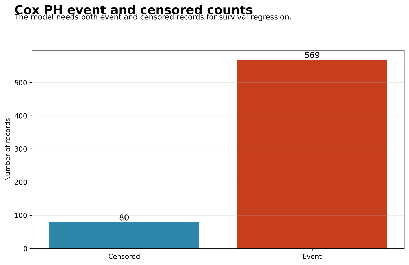
The bars contain 569 records labelled Event and 80 labelled Censored, totaling 649. As displayed, the event share is 87.67% and the censored share is 12.33%. This would provide many observed events for coefficient estimation.
However, the script documentation says event = 1 when G3 < 10. The uploaded status labels should therefore be checked against the generated model-ready CSV. If the 80 records are the G3 < 10 cases, the two bar labels must be reversed before publication.
Python Chart 2: Duration Distribution by Status
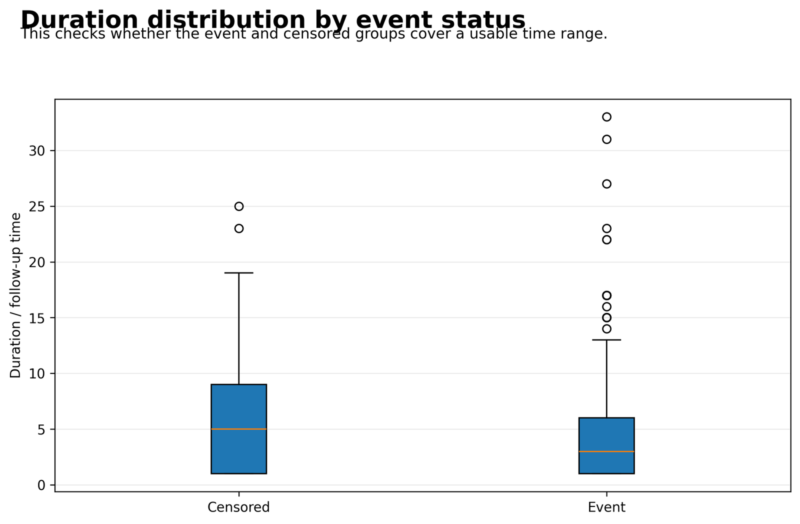
The displayed Censored group has a median duration near 5, with an interquartile range of approximately 1 to 9. Its upper whisker reaches about 19, with outliers near 23 and 25. The displayed Event group has a lower median near 3, an interquartile range of approximately 1 to 6, an upper whisker near 13 and outliers extending to about 33.
Both groups cover multiple duration values, but the distributions are strongly right skewed because duration is based on absences + 1. The long upper tail and many tied integer times should be acknowledged when discussing risk sets and tied-event handling.
Python Chart 3: Hazard-Ratio Forest Plot
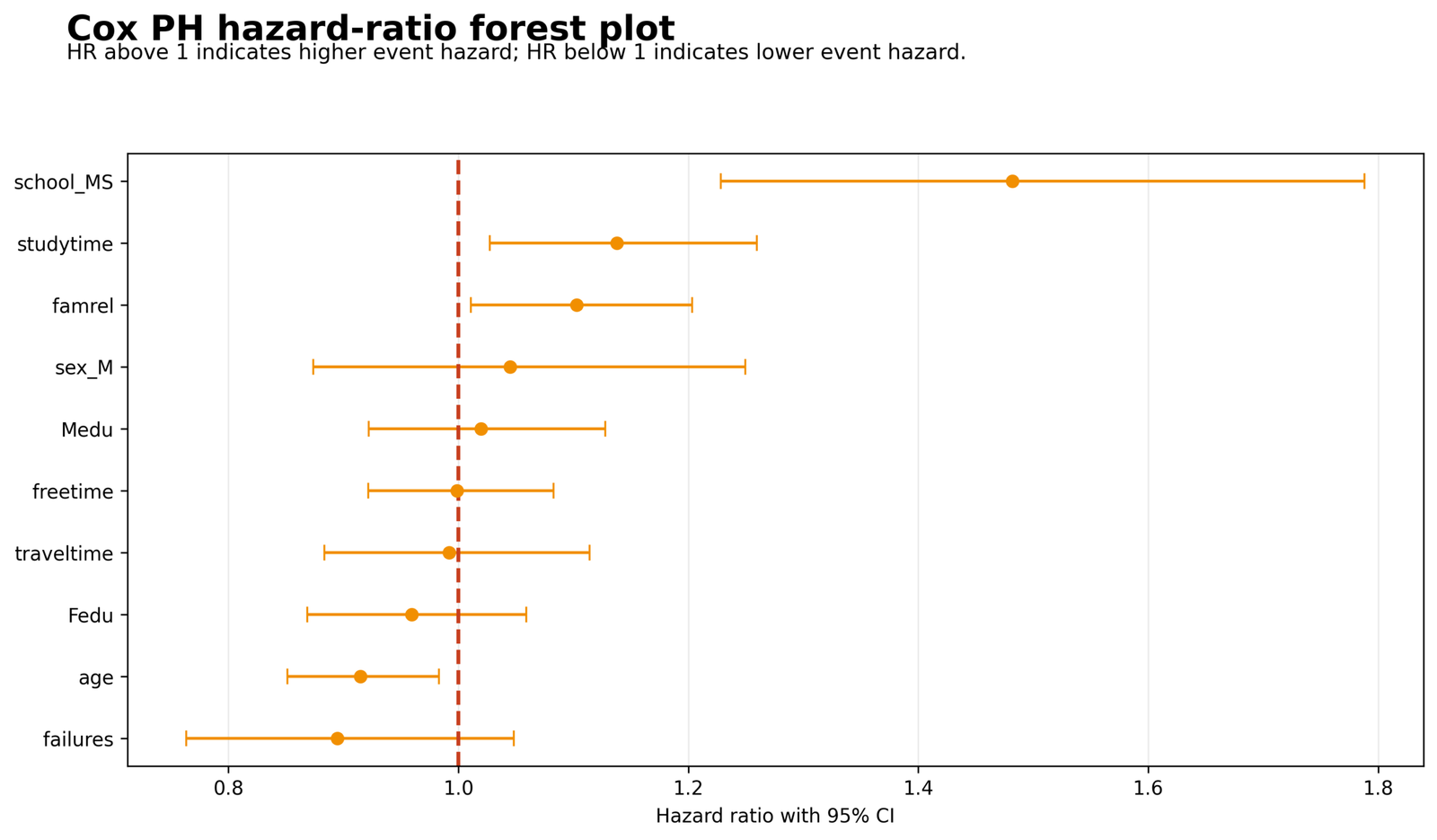
The dashed reference line at HR = 1 separates higher from lower fitted hazard. The largest point is school_MS = 1.4819. Studytime = 1.1377 and famrel = 1.1029 also lie above 1 with intervals fully above the reference. Age = 0.9149 lies below 1 with its interval fully below 1.
Medu, Fedu, traveltime, failures, freetime and sex_M have intervals crossing 1. The forest plot therefore supports four statistically notable terms and six uncertain terms. The direction of these effects must be tied to the verified event definition.
Python Chart 4: Baseline or Overall Survival Curve
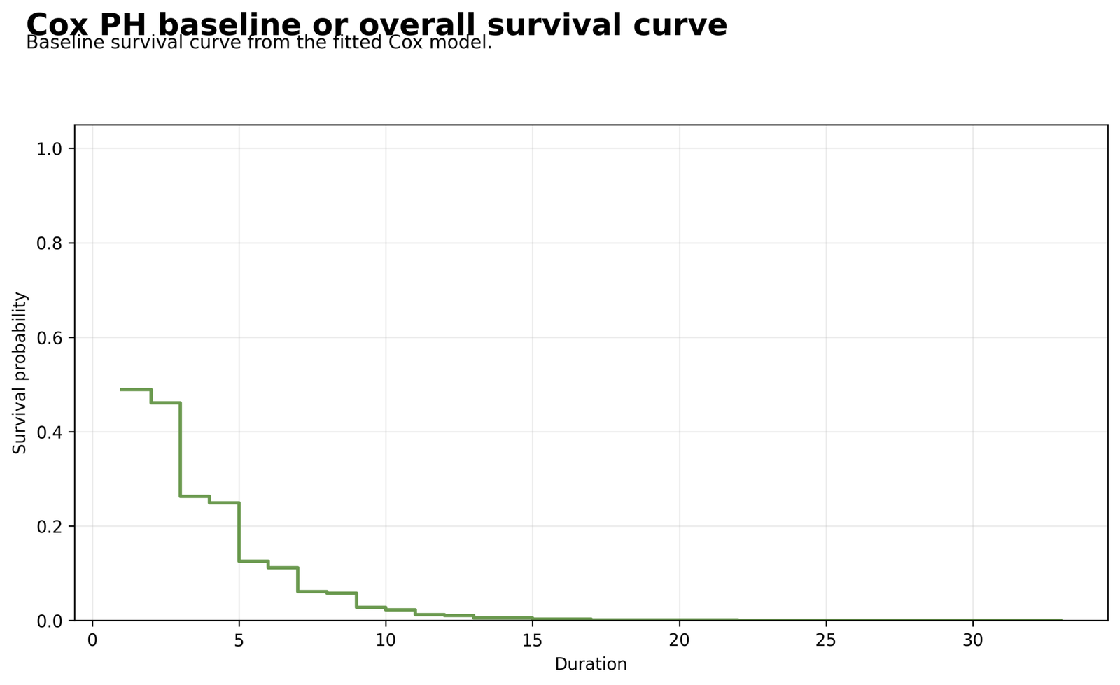
The supplied Python baseline curve begins below 0.50 at the earliest displayed time, falls to roughly 0.26 around duration 3, approximately 0.13 around duration 5, and below 0.05 by about duration 8. It approaches zero after approximately duration 14.
This rapid decline is consistent with the chart’s very large displayed event group. Baseline survival refers to the model’s reference covariate profile; it is not the survival probability for every student. Its unusual starting level also reinforces the need to verify event coding and model centering.
Python Chart 5: Kaplan-Meier Survival by Predicted Risk Group
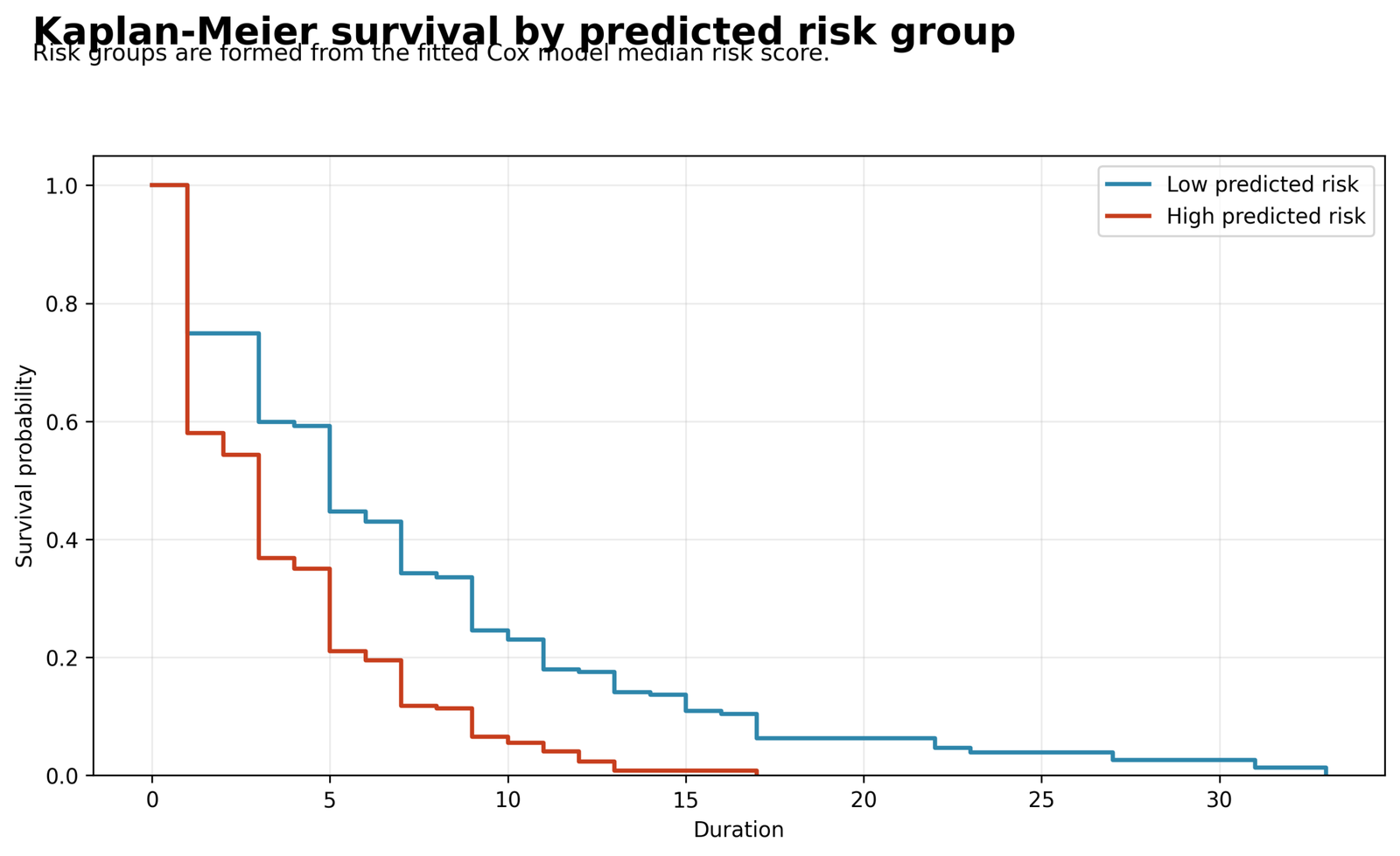
The high-predicted-risk curve falls faster than the low-risk curve. At approximately duration 5, the high-risk survival is near 0.21, compared with about 0.45 in the low-risk group. Around duration 10, the curves are approximately 0.06 and 0.24, respectively.
The high-risk curve reaches almost zero by duration 17, whereas the low-risk group retains a small survival probability into the longest durations. This separation supports practical discrimination, but it is an in-sample median split and is not a substitute for a reported concordance index or external validation.
Python Chart 6: Cumulative Observed Events
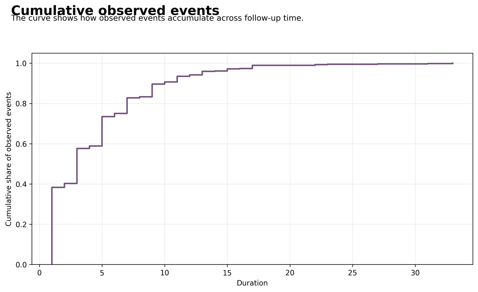
Approximately 38% of displayed events have accumulated by duration 1, about 58% by duration 3, 74% by duration 5, 83% by duration 7 and around 90% by duration 9. The curve exceeds 95% by approximately duration 13 and is nearly complete by duration 17.
The event process is therefore concentrated early on the constructed duration scale. Later observations contribute relatively few additional events, which explains why survival curves flatten close to zero in the tail.
Python Chart 7: Predicted Risk Score Distribution
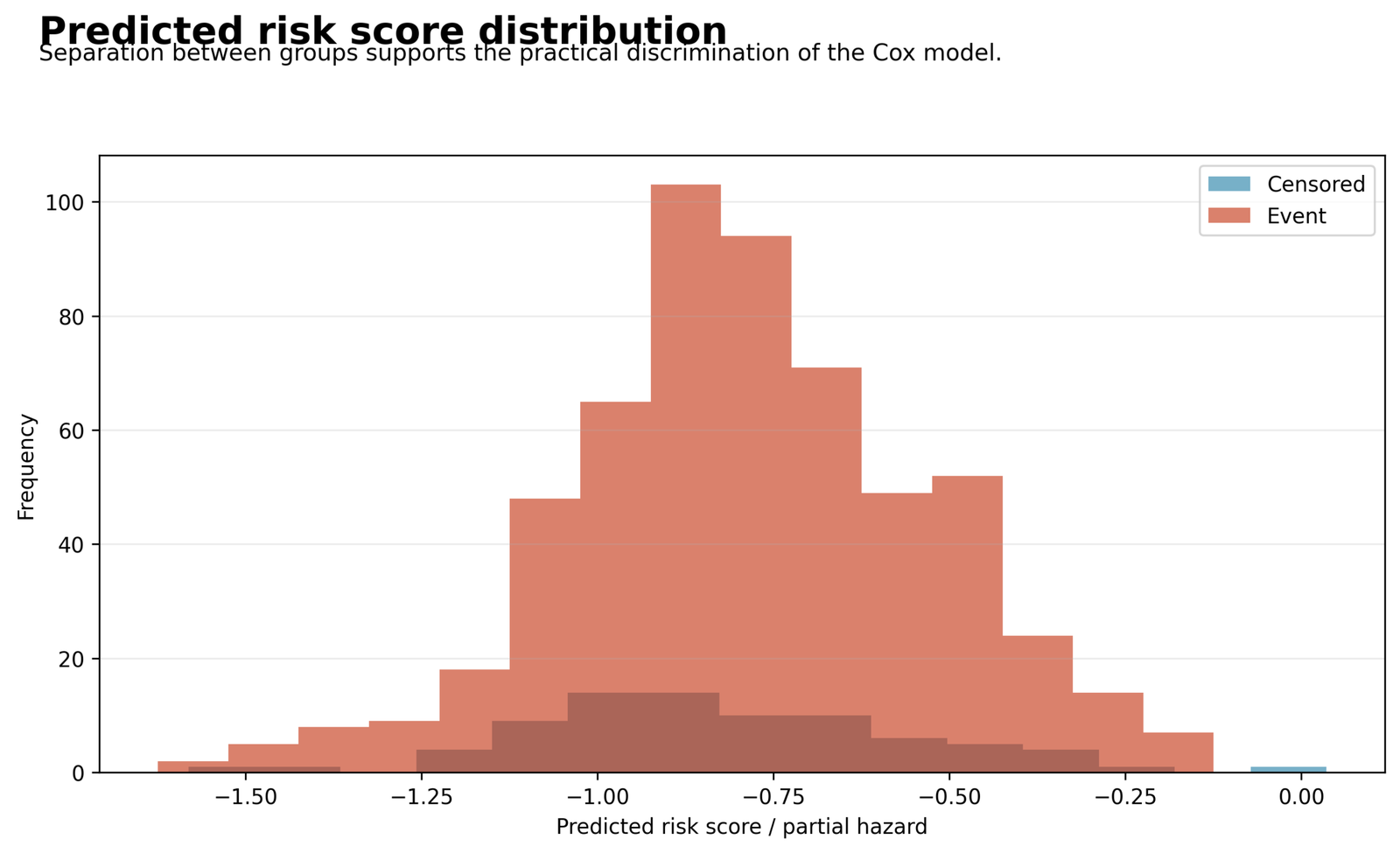
The displayed Event histogram is concentrated mainly between approximately -1.10 and -0.40, with its highest bin slightly above 100 records near -0.9. The displayed Censored group has far fewer records and overlaps substantially with the same risk-score range.
The model separates the groups enough to produce different survival curves, but the overlapping histograms show that discrimination is not perfect. A concordance index and out-of-sample validation would provide a more formal assessment.
Python Chart 8: Hazard-Ratio Summary Table
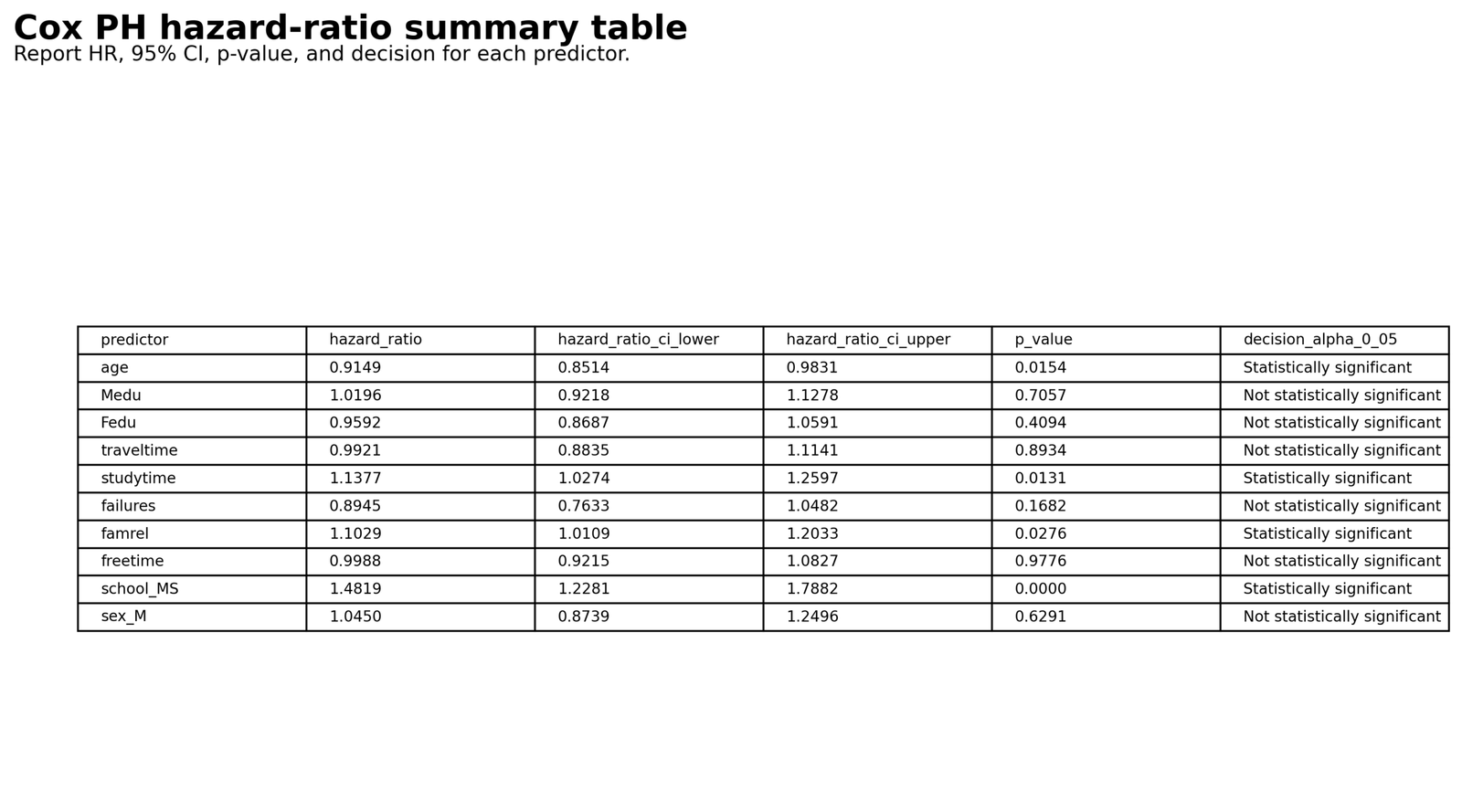
The table confirms the exact values used above. Significant rows are age, studytime, famrel and school_MS. The most precise large effect is school_MS, HR = 1.4819, 95% CI [1.2281, 1.7882]. Freetime is closest to no effect, HR = 0.9988, p = .9776.
This figure should be the primary numeric reference when the forest plot is too compressed to read exact values. It also demonstrates why every chart interpretation should include the underlying numbers rather than only describing point positions.
R Charts and Independent Validation
Open the updated Cox Proportional Hazards Model R report PDF
The R generator fits survival::coxph(), creates a hazard-ratio table and evaluates proportional hazards with cox.zph(). Six confirmed R media URLs are now supplied. The R section now includes the corrected baseline survival chart, Kaplan-Meier curves by predicted risk group, and the Schoenfeld-residual proportional-hazards diagnostic.
R Chart 1: Event and Censored Counts
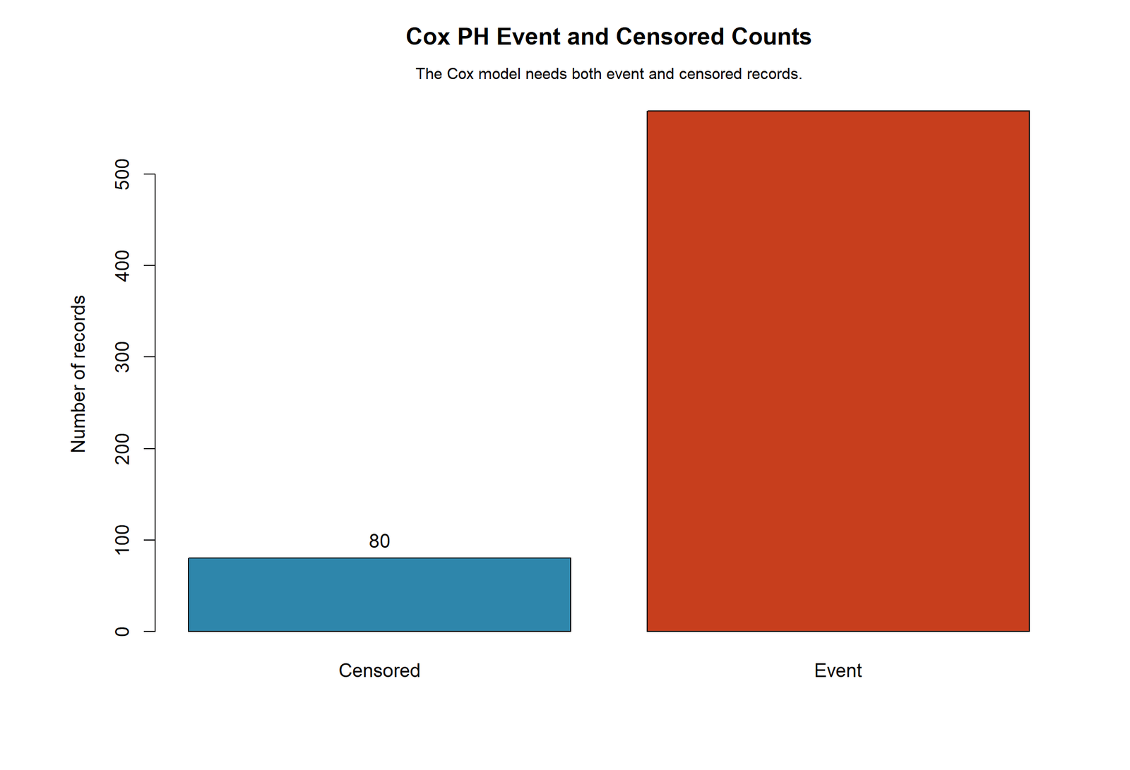
The R count chart visually reproduces the Python values: 569 under Event and 80 under Censored. This cross-software agreement confirms that the same model-ready status values were plotted. It does not resolve whether the labels are correct relative to the documented G3 < 10 coding; the underlying CSV still needs verification.
R Chart 2: Duration Distribution by Status
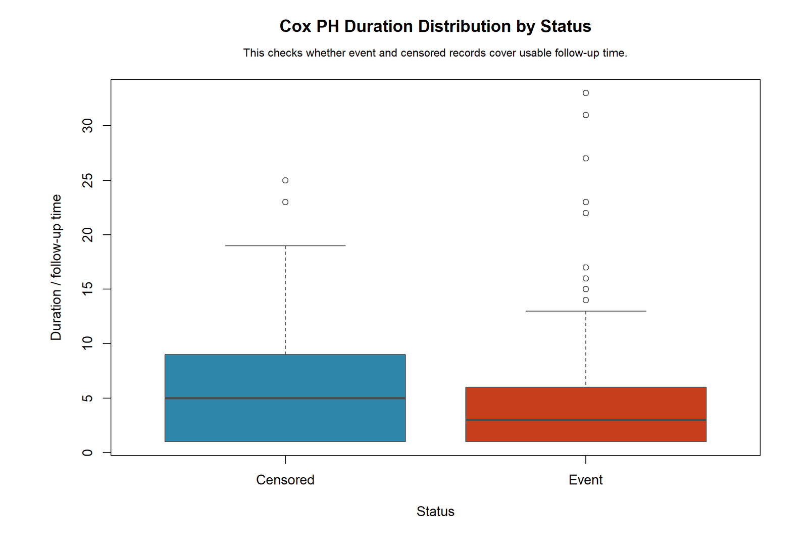
The R boxplot confirms the same approximate medians: 5 for the displayed Censored group and 3 for the displayed Event group. The Event-labelled group has more extreme upper outliers, reaching approximately 33, while the Censored-labelled group reaches about 25.
The agreement between the Python and R boxplots supports the duration summary. The difference is descriptive and should not be interpreted as an adjusted Cox coefficient by itself.
R Chart 3: Hazard-Ratio Forest Plot
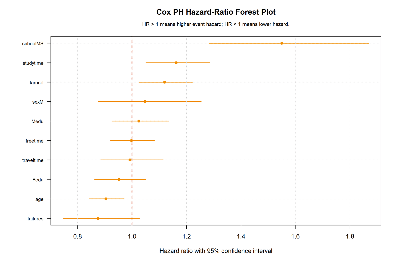
The R forest plot places schoolMS around 1.48, studytime around 1.14, famrel around 1.10 and age around 0.91. It also reproduces the confidence-interval crossings for Medu, Fedu, traveltime, failures, freetime and sexM.
The equivalent predictor labels differ slightly between software, such as school_MS versus schoolMS and sex_M versus sexM. These are naming differences created by dummy coding, not different concepts.
R Chart 4: Baseline Survival with Confidence Limits
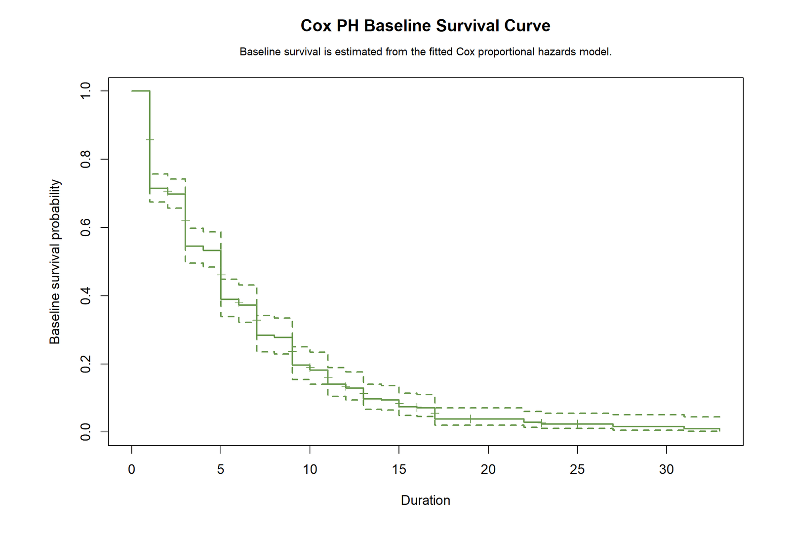
The R baseline survival starts at 1 before the first event, then drops to approximately 0.71 around duration 1, 0.54 around duration 3, 0.38 around duration 5, 0.28 around duration 7 and roughly 0.19 around duration 9. It falls below 0.10 by about duration 14 and approaches zero in the late tail.
The dashed limits widen where fewer observations remain informative. The numerical level differs from the Python baseline figure because baseline curves can depend on implementation details, centering and fitted specification. The hazard-ratio directions are the more directly comparable quantities across the supplied outputs.
R Chart 5: Kaplan-Meier Survival by Predicted Risk Group
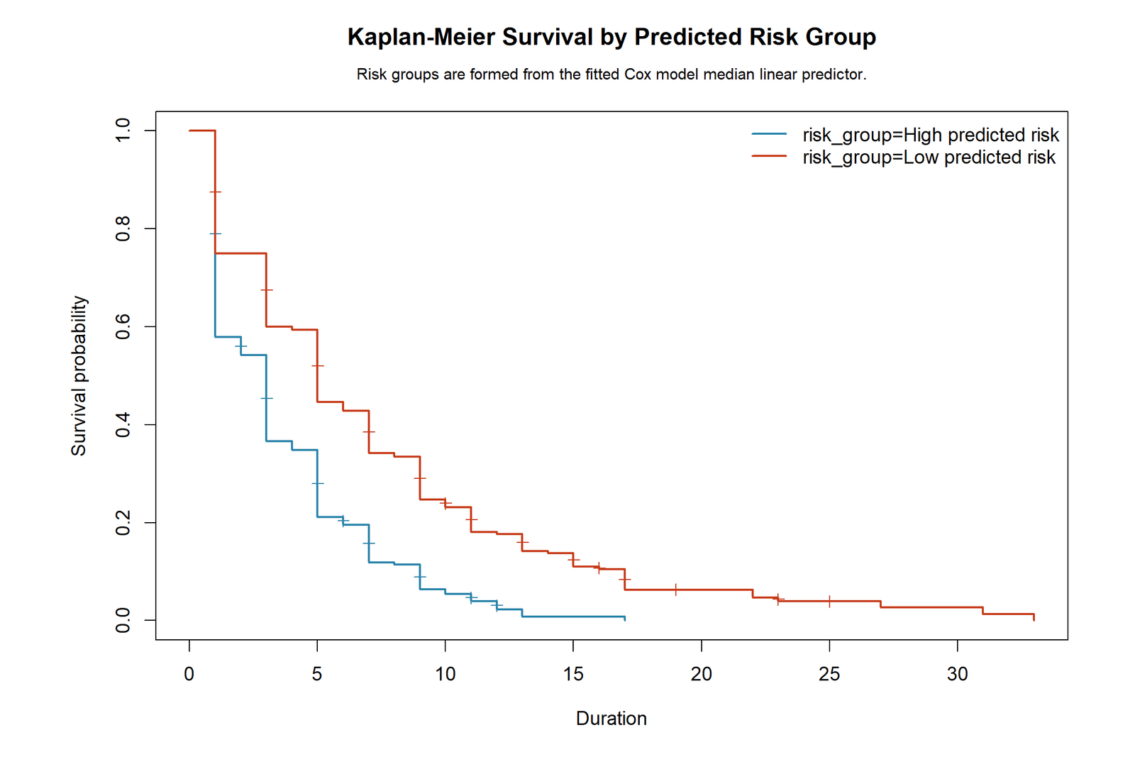
The R Kaplan-Meier chart compares observed survival after the fitted linear-predictor values are divided into lower- and higher-risk groups. The higher-risk curve is expected to decline more rapidly when the Cox risk score discriminates between records with different fitted hazards. In the supplied output, the high-risk curve remains below the low-risk curve across much of the constructed duration scale, matching the separation shown in the Python risk-group chart.
This median-risk split is descriptive and discards some information from the original continuous risk score. Interpret the curve separation together with the hazard-ratio table, confidence intervals, model concordance when available, and the confirmed event coding rather than treating the grouped chart as the primary Cox test.
R Chart 6: Schoenfeld-Residual Proportional-Hazards Check
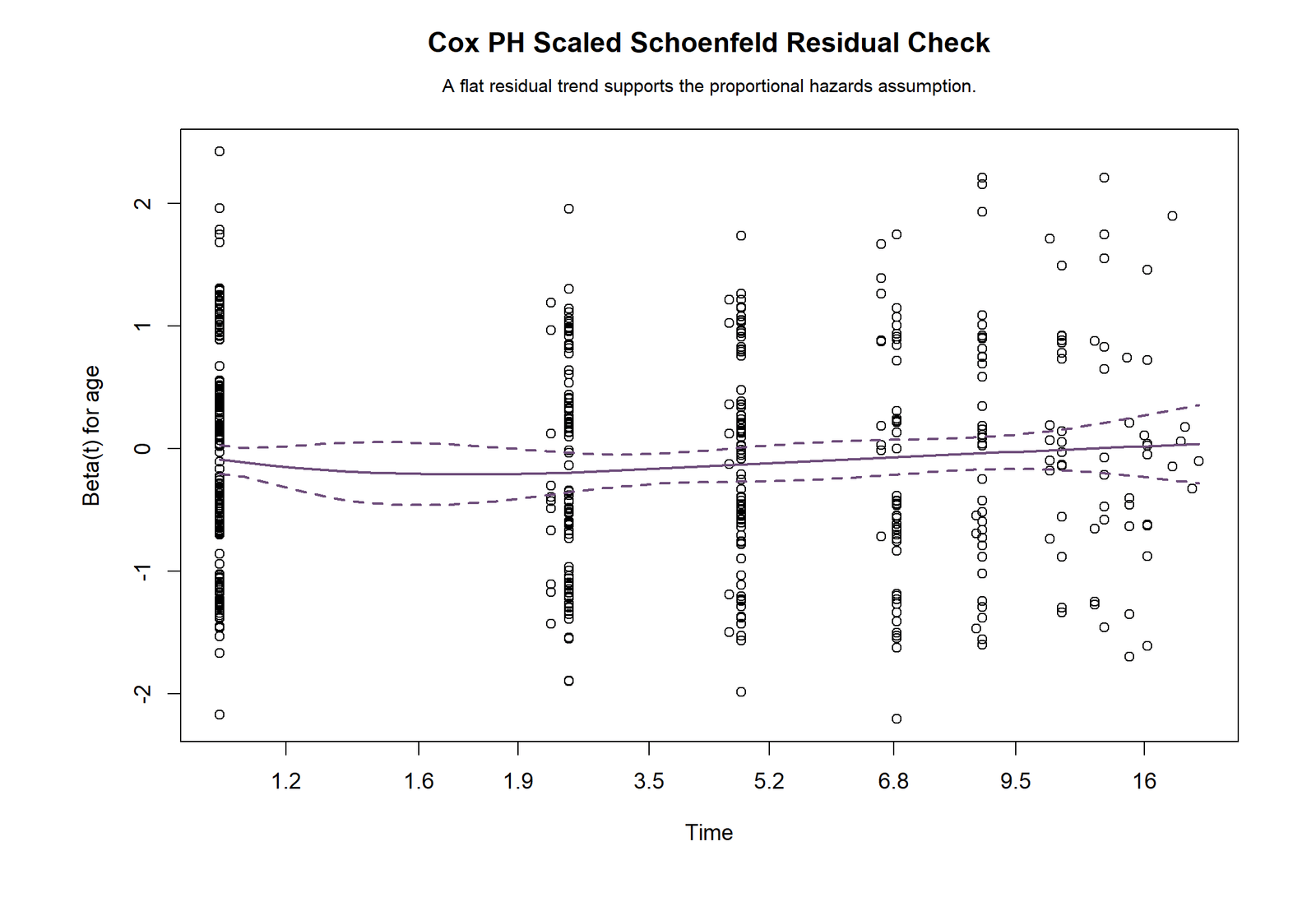
The Schoenfeld-residual chart checks whether the fitted log-hazard effect changes systematically over follow-up time. A smooth pattern that remains approximately horizontal around zero supports the proportional-hazards assumption. Strong curvature, a sustained upward or downward trend, or a small corresponding cox.zph() p-value suggests that the hazard ratio may vary over time.
The visual decision must be read with the numerical cox.zph() results in the updated R report. When a meaningful violation is present, consider a predictor-by-time interaction, a stratified Cox model, a time-varying coefficient model, or another survival specification.
R media update: all six supplied R charts are now embedded, including the corrected baseline-survival image, Kaplan-Meier risk-group chart and Schoenfeld-residual proportional-hazards diagnostic.
SPSS Cox Regression Output Interpretation
The SPSS workflow creates cox_duration = absences + 1, creates cox_event = 1 when G3 < 10, saves the prepared SAV file, runs Kaplan-Meier context and fits a native COXREG model. SPSS reports B, SE, Wald, df, Sig. and Exp(B).
| SPSS Item | What to Read | Interpretation |
|---|---|---|
| Case Processing Summary | Events and censored cases | Verify that the event label and count agree with the intended coding. |
| Variables in the Equation | B, Wald, Sig., Exp(B), 95% CI | Exp(B) is the adjusted hazard ratio. |
| Overall Model Fit | Likelihood-ratio or omnibus statistics | Tests whether the covariate set improves on the null model. |
| Survival / hazard plots | Curve separation and shape | Provide descriptive model context. |
| Log-minus-log plot | Approximate parallelism | Strongly nonparallel curves may indicate a PH problem. |
| Predictor list | Fourteen numeric terms in the supplied syntax | Do not copy the ten-term Python coefficients into this larger SPSS specification. |
Do not use the supplied Binary Logistic Regression SPSS PDF for this post. Cox regression requires time, status, censoring and hazard-ratio output; binary logistic output answers a different question.
Excel Worked Cox Proportional Hazards Results
The Excel workbook is a transparent 20-row teaching example. It contains 10 observed events and 10 censored records, an event rate of 50%, median duration of 6, total partial log-likelihood of -16.6292, mean risk score exp(lp) of 0.1612 and highest-risk row ID 1.
Excel Dashboard
| Excel Metric | Value | Meaning |
|---|---|---|
| Total records | 20 | Small manual example, not the 649-row full model. |
| Observed events | 10 | Rows contributing event terms to the partial likelihood. |
| Censored records | 10 | Rows retained in risk sets until their recorded duration. |
| Event rate | 50% | Balanced teaching example. |
| Median duration | 6 | Middle duration across the 20 rows. |
| Total partial log-likelihood | -16.6292 | Solver objective to maximize. |
| Mean exp(lp) | 0.1612 | Average row-level risk score under the entered coefficients. |
| Highest-risk row | ID 1 | Largest fitted exp(linear predictor) in the example. |
Excel Coefficients and Hazard Ratios
| Predictor | Entered β | EXP(β) | Workbook Interpretation |
|---|---|---|---|
| G1 | -0.08 | 0.9231 | Higher G1 lowers the worked-example hazard by about 7.69% per unit. |
| G2 | -0.12 | 0.8869 | Higher G2 lowers the worked-example hazard by about 11.31% per unit. |
| studytime | -0.05 | 0.9512 | One additional studytime category lowers hazard by about 4.88%. |
| failures | 0.45 | 1.5683 | One additional prior failure increases hazard by about 56.83%. |
Excel Partial-Likelihood Logic
Excel Solver is configured to maximize the total partial log-likelihood by changing the coefficient cells. The workbook is useful for learning the mechanics, but formal confidence intervals, p-values and PH tests should come from Python, R or SPSS.
Python, R, SPSS and Excel Workflows
| Software | Model Specification | Outputs | Important Note |
|---|---|---|---|
| Python | Compact ten-predictor Cox model with dummy-coded school and sex. | Eight charts, hazard-ratio table, PH table, risk scores, TXT and PDF. | Verify event labels in the uploaded chart. |
| R | survival::coxph() using the compact predictor set. | Color charts, coefficient table, model statistics, cox.zph() output and PDF. | Only four R media URLs were supplied. |
| SPSS | Native COXREG with fourteen numeric predictors. | SAV, SPV, PDF, Kaplan-Meier and native survival/hazard plots. | This is not the identical ten-term specification. |
| Excel | 20-row manual partial-likelihood example with four predictors. | Dashboard, row calculations, coefficient cells and Solver instructions. | Teaching workbook, not a replacement for full survival software. |
Cox Proportional Hazards Model Code
Python with lifelines
import pandas as pd
from lifelines import CoxPHFitter
from lifelines.statistics import proportional_hazard_test

df = pd.read_csv("dataset.csv")

# Teaching survival setup
df["cox_duration"] = pd.to_numeric(df["absences"], errors="coerce") + 1
df["cox_event"] = (
    pd.to_numeric(df["G3"], errors="coerce") < 10
).astype(int)

model = df[
    ["cox_duration", "cox_event", "age", "Medu", "Fedu",
     "traveltime", "studytime", "failures", "famrel", "freetime"]
].dropna()

cph = CoxPHFitter(penalizer=0.01)
cph.fit(model, duration_col="cox_duration", event_col="cox_event")
print(cph.summary)

ph_test = proportional_hazard_test(cph, model, time_transform="rank")
print(ph_test.summary)
R with survival
library(survival)

df <- read.csv("dataset.csv", stringsAsFactors = FALSE)
df$cox_duration <- as.numeric(df$absences) + 1
df$cox_event <- ifelse(as.numeric(df$G3) < 10, 1, 0)

fit <- coxph(
  Surv(cox_duration, cox_event) ~
    age + Medu + Fedu + traveltime + studytime +
    failures + famrel + freetime + school + sex,
  data = df,
  ties = "efron",
  x = TRUE
)

summary(fit)
cox.zph(fit)
plot(survfit(fit))
SPSS COXREG Pattern
COMPUTE cox_duration = absences + 1.
COMPUTE cox_event = 0.
IF (G3 < 10) cox_event = 1.
EXECUTE.

COXREG cox_duration WITH
  age Medu Fedu traveltime studytime failures
  famrel freetime goout Dalc Walc health G1 G2
  /STATUS=cox_event(1)
  /METHOD=ENTER age Medu Fedu traveltime studytime failures
    famrel freetime goout Dalc Walc health G1 G2
  /PRINT=CI(95) GOODFIT SUMMARY
  /PLOT SURVIVAL HAZARD LML
  /CRITERIA=PIN(.05) POUT(.10) ITERATE(20).

OUTPUT SAVE OUTFILE=
'D:\DATA ANALYSIS\H Regression Tests and Models\Cox Proportional Hazards Model\SPSS_Output\spv\Cox-Proportional-Hazards-Model-SPSS-Output.spv'.

OUTPUT EXPORT
  /CONTENTS EXPORT=ALL LAYERS=PRINTSETTING MODELVIEWS=PRINTSETTING
  /PDF DOCUMENTFILE=
'D:\DATA ANALYSIS\H Regression Tests and Models\Cox Proportional Hazards Model\SPSS_Output\pdf\Cox-Proportional-Hazards-Model-SPSS-Output.pdf'.
Excel Formulas
Linear predictor:
=SUMPRODUCT(predictor_row, coefficient_cells)
Risk score:
=EXP(linear_predictor)
Risk-set sum:
=SUMIFS(exp_lp_range, duration_range, ">="¤t_duration)
Event partial log-likelihood:
=IF(event_cell=1, linear_predictor-LN(risk_set_sum), 0)
Hazard ratio:
=EXP(coefficient)APA-Style Cox Regression Reporting
Full Report Using the Supplied Hazard-Ratio Table
A Cox proportional hazards model was fitted to a prepared survival outcome with duration defined as absences plus one. The compact Python/R model included age, parental education, travel time, study time, previous failures, family relationship quality, free time, school and sex. The strongest adjusted association was observed for the MS school indicator, HR = 1.482, 95% CI [1.228, 1.788], p < .001. Study time, HR = 1.138, 95% CI [1.027, 1.260], p = .013, and family relationship quality, HR = 1.103, 95% CI [1.011, 1.203], p = .028, were also associated with higher fitted hazard. Age was associated with lower fitted hazard, HR = 0.915, 95% CI [0.851, 0.983], p = .015. The remaining predictor confidence intervals included 1.
Mandatory Coding Qualification
The uploaded count charts displayed 569 events and 80 censored records, whereas the analysis scripts define the event as G3 < 10. The event coding and chart labels must be reconciled before the hazard directions are given a final substantive label such as “higher hazard of low final grade.”
Excel Worked-Example Report
The separate Excel workbook demonstrated Cox partial-likelihood calculations using 20 records, 10 events and 10 censored observations. Entered coefficients produced hazard ratios of 0.923 for G1, 0.887 for G2, 0.951 for studytime and 1.568 for failures. The total partial log-likelihood was -16.629. These are manual teaching values rather than estimates from the 649-row Cox model.
Common Cox Regression Mistakes
| Mistake | Why It Is Wrong | Correct Practice |
|---|---|---|
| Reversing event and censor codes | Hazard directions and event counts become misleading. | Verify that 1 is the intended event and 0 is censoring in every file and chart. |
| Calling HR a probability ratio | Hazard is an instantaneous rate concept. | Describe HR as a multiplicative hazard comparison. |
| Ignoring the 95% CI | A point estimate alone does not show uncertainty. | Report HR, interval and p-value together. |
| Skipping PH checks | A constant hazard ratio over time is a central model assumption. | Use Schoenfeld tests, residual plots and time interactions. |
| Discarding censored cases | Censored observations contribute risk-set information. | Retain them with event/status = 0. |
| Mixing Python/R and SPSS coefficients | The supplied specifications contain different predictor sets. | Report each software model separately unless specifications are identical. |
| Using the Binary Logistic Regression PDF | Logistic regression ignores follow-up time and censoring. | Use only Cox-specific SPSS/R/Python output. |
| Treating the constructed student outcome as a natural survival endpoint | Absences and grade status are teaching transformations. | State the construction clearly and use genuine follow-up variables in substantive research. |
Cox Regression Reporting Checklist
A high-quality report should allow another analyst to reconstruct the survival outcome, predictor coding and model decisions. The following checklist is more useful than reporting only a forest plot.
| Reporting Element | Required Information | Why It Matters |
|---|---|---|
| Time variable | Name, units, minimum, maximum and construction rule. | Defines the survival scale and risk-set ordering. |
| Event variable | Exact meaning of 1 and 0. | Prevents reversal of hazard interpretation. |
| Censoring | Number and percentage censored, plus reason where known. | Shows the effective information structure. |
| Sample size | Total records and complete cases used. | Clarifies exclusions and missing-data handling. |
| Predictors | Names, units, dummy references and transformations. | Makes hazard ratios interpretable. |
| Tie method | Efron, Breslow or exact. | Supports software reproducibility. |
| Model fit | Likelihood-ratio, Wald or score statistic. | Shows whether the model improves on the null. |
| Discrimination | Concordance index with validation approach. | Evaluates risk ranking. |
| Coefficient results | B, SE, HR, 95% CI and p-value. | Provides effect magnitude and uncertainty. |
| PH diagnostics | Schoenfeld tests, global test and plots. | Evaluates the central model assumption. |
| Functional form | Assessment of nonlinear continuous effects. | Prevents misleading one-unit HR estimates. |
| Validation | Internal resampling or external dataset when prediction is a goal. | Reduces optimism in performance estimates. |
Recommended Results Order
Begin with the sample and event/censoring summary. Next report overall model fit, followed by hazard ratios with confidence intervals. Then present proportional-hazards diagnostics, discrimination, survival curves and sensitivity analyses. Keep the substantive conclusion tied to the event definition and reference categories.
Recommended Limitations Wording for This Teaching Example
The survival duration and event status were constructed from educational variables rather than collected as a natural longitudinal endpoint. The analysis is therefore intended to demonstrate Cox-regression mechanics. Event coding and the uploaded event/censor labels should be reconciled before interpreting the hazard direction substantively.
Cox Regression Troubleshooting Guide
Model Does Not Converge
Nonconvergence may result from complete separation, an extremely sparse category, severe multicollinearity, too many predictors for the number of events or a predictor with almost no variation. Inspect category counts, coefficient magnitude and warnings. Simplify the model or use penalization when appropriate.
Very Large Hazard Ratios or Confidence Intervals
Extreme hazard ratios often reflect sparse data, near separation, unstable dummy categories or poor scaling. Report the instability rather than presenting the point estimate as a precise effect. Combining categories should be based on subject knowledge, not only on obtaining smaller coefficients.
Confidence Interval Includes 1 but p-Value Appears Significant
This is usually caused by rounding or by using statistics from different models. Use more decimal places and confirm that the coefficient, standard error, p-value and interval all come from the same fitted specification.
Python, R and SPSS Results Differ
First compare event coding, censor value, predictor list, reference categories, missing-data exclusions, tie method, penalization and continuous-variable scaling. In the supplied files, Python/R and SPSS already use different predictor specifications, so identical coefficients should not be expected.
Baseline Survival Curves Differ Across Software
Baseline curves may differ because software centers predictors differently or reports survival for different reference profiles. Hazard ratios can agree while baseline survival levels differ. Document the covariate profile associated with each curve.
Global PH Test Is Significant
Inspect predictor-specific tests and plots rather than immediately rejecting the entire model. Identify which terms drive the result, evaluate practical magnitude, test time interactions and compare alternative specifications.
Too Few Events for the Predictor Count
Reduce unnecessary terms, combine carefully justified variables, use penalized methods or collect more event information. The relevant information is closer to the event count than the total sample size. A large number of censored records does not fully compensate for very few events.
Risk Groups Do Not Separate
Weak risk-group separation may indicate low discrimination, an arbitrary cut point, incorrect event coding or overfitting. Report the concordance index and consider continuous calibration rather than relying solely on a median split.
Downloads and Resources
Link verification: the updated R report URL is confirmed and included below. The Python report, SPSS report and Excel workbook URLs still follow the generator filenames and should be confirmed in WordPress Media. The unrelated binary-logistic report URLs have not been used.
Updated R Cox Report PDFConfirmed R report with hazard ratios, survival charts and proportional-hazards diagnostics.
SPSS Cox Output PDFExpected native COXREG Viewer export filename.
Worked Excel FileExpected WordPress filename for the 20-row partial-likelihood workbook.
FAQs About Cox Proportional Hazards Models
What is a Cox proportional hazards model?
It is a survival-regression model that estimates how predictors multiply the instantaneous event hazard while retaining right-censored records.
How do I interpret a hazard ratio?
HR above 1 indicates higher fitted event hazard, HR below 1 indicates lower fitted event hazard and HR equal to 1 indicates no fitted hazard difference.
Which predictors were significant in the supplied compact model?
Age, studytime, famrel and school_MS had 95% hazard-ratio confidence intervals that did not include 1.
What was the strongest hazard ratio?
school_MS had HR = 1.4819, 95% CI [1.2281, 1.7882], p < .0001.
How many events and censored records were shown?
The supplied charts displayed 569 Event records and 80 Censored records. The script coding appears inconsistent with those labels and must be verified before publication.
What is the proportional hazards assumption?
It assumes that the hazard ratio associated with a predictor is reasonably constant across follow-up time. Schoenfeld residual tests and time-interaction checks are commonly used.
Can Cox regression be performed in SPSS?
Yes. SPSS uses COXREG with a duration variable, status variable and covariates. Report Exp(B) with its 95% confidence interval.
Can Cox regression be calculated in Excel?
Excel can demonstrate risk scores and partial-likelihood contributions, and Solver can optimize coefficients. Full inference and PH diagnostics are safer in Python, R or SPSS.
Why is the Excel result different from Python and R?
The workbook contains only 20 teaching rows and four entered coefficients. The full model contains 649 records and a different predictor specification.
Is Cox regression the same as binary logistic regression?
No. Logistic regression models event probability without follow-up time or censoring. Cox regression models event hazard over time and retains censored observations.
Final Cox Proportional Hazards Model Conclusion
The supplied compact Cox model identifies school_MS as the strongest hazard-ratio term, followed by smaller significant effects for studytime, famrel and age. The Python and R media agree on the hazard-ratio pattern, duration distributions and displayed 569-to-80 status split. The Excel workbook separately demonstrates how risk scores and partial likelihood are calculated.
The final publishing step is to correct or confirm the event/censor labels. Once event = 1 is verified consistently in the model-ready data, count charts, survival curves and software reports, the hazard directions can be given a definitive substantive interpretation.

