
Adjusted Goodness of Fit Index (AGFI): Formula, Interpretation, R, Python, SPSS and Excel
The Adjusted Goodness of Fit Index is an absolute structural equation modeling fit index that adjusts GFI for model complexity. This complete guide explains the actual AGFI formula, model identification, assumptions, a verified two-factor CFA example, residual diagnostics, reporting, and reproducible workflows in R, Python, SPSS AMOS and Excel.
AGFI = .981 indicates strong adjusted global fit for the worked CFA model.
For the verified two-factor model, GFI = 0.9926350186, p = 6 observed variables and df = 8. The model contains 21 unique covariance moments and 13 free parameters. Applying the degrees-of-freedom adjustment gives AGFI = 0.9806669237, conventionally reported as AGFI = .981.
What does the Adjusted Goodness of Fit Index measure?
A global covariance-fit index with an explicit complexity adjustment.
Across R, Python, SPSS AMOS and Excel, AGFI should be treated as one member of a model-fit profile. SEM software can return it beside chi-square, CFI, TLI, RMSEA and SRMR, while the same model object supplies residuals and standardized estimates. This makes it easy to avoid a common reporting error: selecting the most favorable index and ignoring contradictory evidence.
AGFI adjusts GFI for model parsimony. A model that reproduces the covariance matrix well but estimates many parameters has fewer degrees of freedom available for testing. The adjustment therefore acts on the GFI shortfall from one. It does not reward complexity simply because the raw GFI rose after paths were freed.
The worked model contains two correlated latent variables. Academic is measured by G1, G2 and G3; Social is measured by famrel, freetime and goout. With six observed indicators and thirteen free parameters, the fitted model reports eight degrees of freedom. The analysis is deliberately overidentified so global fit can be assessed.
What AGFI answers
AGFI asks how closely the fitted covariance structure reproduces the observed covariance structure after the raw GFI lack-of-fit is expanded by a degrees-of-freedom factor. It is an absolute fit index, because it evaluates the proposed model’s reproduction of the data rather than only comparing it with an independence model.
The result belongs to the entire specified model. It does not identify which loading, residual variance or factor covariance is responsible for fit. For local evidence, examine residuals, standardized estimates and theoretically meaningful misspecification. Continue with correlation assumptions when the observed association structure needs a preliminary audit.
What AGFI does not answer
AGFI is not a reliability coefficient, a validity coefficient, a variance-explained percentage or a direct test that every parameter is correct. A high value does not establish convergent validity, discriminant validity, causal direction or measurement invariance.
Reliability evidence for the indicators must be assessed separately through tools such as Cronbach’s alpha and McDonald’s omega. Likewise, global covariance fit cannot replace substantive evaluation of the factor definitions.
Why AGFI must be interpreted with model complexity
The same GFI can produce a different AGFI when model degrees of freedom change.
The Adjusted Goodness of Fit Index does not evaluate covariance reproduction in isolation. It begins with the model’s GFI shortfall and expands that shortfall according to the ratio of observed covariance moments to model degrees of freedom. The same GFI can therefore lead to different AGFI values when two models estimate different numbers of parameters.
What controls the adjustment
Three quantities determine the calculation: the number of observed variables, the fitted model’s degrees of freedom and GFI. With six observed variables, this analysis contains 21 unique variances and covariances. Thirteen free parameters leave eight degrees of freedom, so the GFI shortfall is multiplied by .
Because GFI = 0.9926350186, its shortfall from one is 0.0073649814. Applying the complexity multiplier increases the shortfall to 0.0193330763 and produces AGFI = 0.9806669237. the fitted-model output and the independent formula check must agree on all of these values.
What a high AGFI does not establish
AGFI = .981 supports strong adjusted global covariance fit for this specified model, but it does not prove that the factor structure is uniquely correct. It does not establish reliability, convergent validity, discriminant validity, causal direction, measurement invariance or the absence of local misspecification.
The residual-correlation matrix still contains nonzero discrepancies, and the social-indicator block is substantially weaker than the academic block. Those findings remain relevant even when the global adjusted index is high.
| Interpretation question | Required evidence | Current analysis |
|---|---|---|
| Is the model overidentified? | Positive model degrees of freedom | Yes; df = 8 |
| Can the AGFI arithmetic be reproduced? | p, observed moments, free parameters, df and full-precision GFI | 6 variables, 21 moments, 13 parameters and GFI = 0.9926350186 |
| Does global fit remove the need for local checks? | Residual matrix, standardized estimates and parameter plausibility | No; residual correlations are reviewed separately |
| Can this value be transferred to another model? | Identical data, variables, estimator, constraints and missing-data treatment | No; AGFI belongs only to this fitted specification |
Worked two-factor CFA model and data dictionary
Every fit index belongs to a specific model, estimator and analysis sample.
The worked analysis uses 649 complete cases from a student-performance dataset. The measurement model defines an Academic factor using G1, G2 and G3 and a Social factor using famrel, freetime and goout. The two factors are correlated. This exact specification generates the GFI, AGFI and residual matrix reported throughout the post.
| Variable | Role in CFA | Scale and interpretation | Observed relationship context |
|---|---|---|---|
| G1 | Academic indicator | First-period grade, numeric | Strongly correlated with G2 and G3 |
| G2 | Academic indicator | Second-period grade, numeric | Largest academic correlation with G3 |
| G3 | Academic indicator | Final grade, numeric | Outcome-like grade used here as an indicator |
| famrel | Social indicator | Family relationship quality, ordered numeric | Weak positive relation with freetime and goout |
| freetime | Social indicator | Free time after school, ordered numeric | Correlation with goout = .346 |
| goout | Social indicator | Going-out frequency, ordered numeric | Completes the social measurement block |
Academic block
The correlations among G1, G2 and G3 are .865, .826 and .919. The supplied SPSS output reports Cronbach’s alpha = .951 and standardized alpha = .953 for these three indicators. Those values describe internal consistency, not CFA fit, but they help explain why a common academic factor is plausible.
Review Cronbach’s alpha interpretation and item-total correlation before claiming that high factor fit alone establishes scale quality.
Social block
The social indicators are much less homogeneous: famrel–freetime = .129, famrel–goout = .090 and freetime–goout = .346. The supplied SPSS reliability output gives alpha = .419 for this block. The two-factor model can still reproduce the covariance matrix globally, but the weak block reliability requires substantive caution.
This contrast is a major reason the article reports residuals and reliability context rather than presenting AGFI = .981 as a complete validation statement.
Adjusted Goodness of Fit Index formula in actual mathematical form
The complete expression connects GFI, observed covariance moments and model degrees of freedom.
Here p is the number of observed variables and df is the degrees of freedom of the fitted covariance model. Because is the number of unique variances and covariances, the bracketed term is the ratio of observed moments to available model df.
GFI shortfall
1 − GFI is the raw lack-of-fit amount on the GFI scale. In this analysis it equals 0.0073649814.
Complexity multiplier
. Fewer degrees of freedom produce a larger multiplier and therefore a stronger adjustment.
Adjusted shortfall
2.625 × 0.0073649814 = 0.0193330763. Subtracting this from one gives AGFI.
The full-precision value is used for verification. Report AGFI = .981 in prose unless a journal or technical appendix requires additional decimals.
Unlike the site’s statistical calculator guides, this index cannot be interpreted from a formula alone. The GFI input must come from a correctly estimated covariance model, and the df must correspond to that same model.
Observed moments, free parameters and model identification
AGFI is not interpretable until the model degrees of freedom are verified.
| Identification quantity | Formula or count | Worked value | Interpretive role |
|---|---|---|---|
| Observed variables | p | 6 | Six measured indicators enter the covariance matrix |
| Observed moments | 21 | Six variances plus fifteen unique covariances | |
| Free loadings | Two marker loadings fixed | 4 | Two additional loadings per factor are estimated |
| Factor variances | One per factor | 2 | Academic and Social variances |
| Factor covariance | Academic ~~ Social | 1 | The latent factors are allowed to correlate |
| Residual variances | One per observed variable | 6 | Indicator-specific variance |
| Total free parameters | 4 + 2 + 1 + 6 | 13 | Model-implied covariance parameters |
| Model df | 21 − 13 | 8 | Positive df makes global fit testable |
Any change to the model can alter this ledger. Adding a cross-loading, residual covariance or free factor path usually increases the parameter count and lowers df. Equality constraints can increase df. Therefore, model modification must be accompanied by a new identification table, not merely a new fit index.
AGFI assumptions and prerequisites
Check estimation, identification, data quality and admissibility before interpreting fit.
Correct model identification
The specified CFA must be identified, converge, and yield an admissible solution. Negative variances, impossible correlations or nonpositive-definite matrices invalidate a simple fit-index reading.
Appropriate measurement level
The estimator must match the observed variables. Treating strongly ordinal indicators as continuous under ordinary ML can distort covariance fit.
Independent observations
Rows should represent independent units unless the model and estimator account for clustering, repeated observations or complex sampling.
Defensible missing-data handling
Listwise deletion, FIML and imputation can produce different covariance structures. State the method and analysis N.
Theoretically specified factor structure
Fit indices cannot rescue an arbitrary measurement model. Factor membership, correlated errors and cross-loadings need substantive justification.
Adequate distribution and estimator
Multivariate nonnormality can affect chi-square and fit statistics. Robust estimators or bootstrap procedures may be needed.
Preliminary distribution checks can use goodness-of-fit testing, Shapiro-Wilk test and the broader Correlation assumptions guide, but those procedures do not substitute for SEM-specific residual and estimator diagnostics.
Worked AGFI calculation: from GFI to AGFI
Every intermediate value is shown so the result can be reproduced outside any software package.
| Step | Calculation | Exact or working value | Meaning |
|---|---|---|---|
| 1 | Unique observed covariance moments | ||
| 2 | AGFI complexity multiplier | ||
| 3 | 1 − GFI | 1 − 0.9926350185704358 = 0.0073649814295642 | Unadjusted GFI shortfall |
| 4 | multiplier × shortfall | 2.625 × 0.0073649814295642 = 0.0193330762526061 | Adjusted shortfall |
| 5 | 1 − adjusted shortfall | 1 − 0.0193330762526061 = 0.980666923747394 | Final AGFI |
The analysis report gives 0.9806667285 and the Python/SPSS verification gives 0.9806669237. The difference is approximately two ten-millionths and is consistent with tiny differences in the stored GFI or computational path. Both round to .981.
Adjusted Goodness of Fit Index in R with lavaan
Fit the CFA, extract AGFI and inspect the residual correlation matrix from one reproducible model object.
R provides an unusually clean audit trail because the same fitted lavaan object can return fit indices, parameter estimates, residuals, modification indices and sample statistics. The safest workflow stores the model syntax as text, fixes the analysis variable set before estimation, requests AGFI explicitly through fitMeasures(), and saves both the exact result and a rounded reporting value.
Freeze the variable set
Create a six-column data frame and document complete-case handling before fitting the model.
Write lavaan syntax explicitly
Specify both measurement blocks and the factor covariance in a stored character string.
Estimate the CFA
Use cfa() with a declared estimator and request convergence information.
Request AGFI by name
Use fitMeasures(fit, c(“gfi”,”agfi”,”df”)) rather than searching a long printed summary.
Audit identification
Verify 21 observed moments, thirteen free parameters and eight degrees of freedom.
Review residuals and estimates
Inspect residual correlations, standardized loadings, factor correlation and any theoretically defensible modification evidence.
Quality-control checkpoint
Before reporting AGFI, confirm that N = 649, p = 6, observed moments = 21, free parameters = 13, df = 8 and GFI is stored at full precision. A mismatch in any one item means the final index belongs to a different analysis.
library(lavaan)dat <- read.csv("dataset.csv")
vars <- c("G1", "G2", "G3", "famrel", "freetime", "goout")
dat <- dat[complete.cases(dat[vars]), vars]
model <- '
Academic =~ G1 + G2 + G3
Social =~ famrel + freetime + goout
Academic ~~ Social
'
fit <- cfa(model, data = dat, estimator = "ML")
fitMeasures(fit, c("df", "gfi", "agfi", "cfi", "tli", "rmsea", "srmr"))
resid(fit, type = "cor")
Adjusted Goodness of Fit Index in R troubleshooting
| Problem | Likely cause or meaning | Recommended action |
|---|---|---|
| lavaan returns NA for AGFI | Check identification, estimator support, convergence and whether the requested fit measure exists for the fitted object. | Recheck the model specification, df, estimator, full-precision inputs and documented software behavior before reporting. |
| AGFI changes after adding a residual covariance | That modification changes both fit and the free-parameter count. Recalculate df and interpret the change as a new model, not a cosmetic improvement. | Recheck the model specification, df, estimator, full-precision inputs and documented software behavior before reporting. |
| The R value differs slightly from Python | Small differences can result from optimizer tolerance, covariance divisor, package formulas or printed precision. Compare the same model and full-precision values. | Recheck the model specification, df, estimator, full-precision inputs and documented software behavior before reporting. |
| fitMeasures() looks good but residuals remain structured | Global fit can hide localized misspecification. Use residuals, standardized loadings and theory together. | Recheck the model specification, df, estimator, full-precision inputs and documented software behavior before reporting. |
| The model uses ordinal indicators | Use an estimator designed for ordered data and report the fit family returned for that estimator rather than forcing an ML AGFI interpretation. | Recheck the model specification, df, estimator, full-precision inputs and documented software behavior before reporting. |
Adjusted Goodness of Fit Index in Python with semopy
Estimate the model, extract the fit table and verify AGFI with transparent Python arithmetic.
Python is strongest here when the fitted-model output and the transparent arithmetic are kept in the same notebook. semopy estimates the CFA and supplies fit indices; pandas controls the analysis sample; NumPy can reconstruct residual matrices; and a short independent formula check catches group, parameter-count or column-selection errors before the result reaches a report.
Prepare a fixed analysis frame
Select only G1, G2, G3, famrel, freetime and goout before complete-case deletion. This prevents unrelated columns from changing the sample size.
Declare the measurement model
Use a plain-text semopy description with two factors and an explicit factor covariance. Save the exact string with the report.
Fit and verify convergence
Inspect the optimizer result, objective value and parameter table. Do not calculate fit measures from a failed or nonconverged model.
Extract the complete fit profile
Use calc_stats() and retain DoF, GFI, AGFI, CFI, TLI, RMSEA, chi-square and baseline-model quantities.
Rebuild AGFI manually
Calculate observed moments and the penalty multiplier from p and df. Compare the reconstructed value with the package output.
Inspect local residuals
Compute or extract the residual covariance/correlation matrix and rank absolute off-diagonal entries.
Quality-control checkpoint
Before reporting AGFI, confirm that N = 649, p = 6, observed moments = 21, free parameters = 13, df = 8 and GFI is stored at full precision. A mismatch in any one item means the final index belongs to a different analysis.
import pandas as pd
from semopy import Model, calc_statsdata = pd.read_csv("dataset.csv")
cols = ["G1", "G2", "G3", "famrel", "freetime", "goout"]
data = data[cols].dropna().copy()
model_desc = """
Academic =~ G1 + G2 + G3
Social =~ famrel + freetime + goout
Academic ~~ Social
"""
model = Model(model_desc)
result = model.fit(data)
stats = calc_stats(model)
print(stats.loc["Value", ["DoF", "GFI", "AGFI", "CFI", "TLI", "RMSEA"]])
Adjusted Goodness of Fit Index in Python troubleshooting
| Problem | Likely cause or meaning | Recommended action |
|---|---|---|
| AGFI is missing from the output | Confirm that calc_stats(model) was called after a successful fit and that the returned table is indexed by Value. | Recheck the model specification, df, estimator, full-precision inputs and documented software behavior before reporting. |
| AGFI differs from the manual worksheet | Check whether the Python package uses baseline-model df rather than , whether means are estimated, and whether the same GFI is being adjusted. | Recheck the model specification, df, estimator, full-precision inputs and documented software behavior before reporting. |
| The model has zero or negative df | Reduce free parameters or revise the model. AGFI is not meaningful for a saturated or underidentified specification. | Recheck the model specification, df, estimator, full-precision inputs and documented software behavior before reporting. |
| Results change after dropna() | Document the complete-case variables. Dropping rows on additional columns silently changes N and the covariance matrix. | Recheck the model specification, df, estimator, full-precision inputs and documented software behavior before reporting. |
| Residuals look large despite AGFI above .95 | Treat this as local misfit. Inspect the particular indicator pairs, modification evidence and theory rather than relying on the global index. | Recheck the model specification, df, estimator, full-precision inputs and documented software behavior before reporting. |
Adjusted Goodness of Fit Index in SPSS AMOS
Use SPSS Statistics for screening and Amos for the confirmatory covariance model and fit indices.
A correct SPSS workflow distinguishes three tasks. SPSS Statistics imports, labels, screens and saves the observed variables. Amos specifies and estimates the latent-variable model. A separate arithmetic cross-check verifies the relationship among GFI, AGFI, p and df. Treating these tasks as one menu click is the main reason many online explanations confuse exploratory factor analysis with confirmatory model fit.
Audit the data in SPSS Statistics
Confirm 649 rows, numeric measurement levels, missing values and the six-variable correlation matrix.
Open the Amos model
Create two latent factors, attach three indicators to each, correlate the factors and identify each measurement block.
Set analysis properties
Choose the estimator and missing-data strategy deliberately. Mean/intercept estimation affects availability of traditional GFI-family output.
Run Calculate Estimates
Check that Amos reports a successful solution and no identification or admissibility warnings.
Open Model Fit → RMR, GFI
Record GFI and AGFI with df and the rest of the model-fit profile.
Cross-check independently
Use the displayed GFI, p = 6 and df = 8 in SPSS or Excel to reproduce AGFI.
Quality-control checkpoint
Before reporting AGFI, confirm that N = 649, p = 6, observed moments = 21, free parameters = 13, df = 8 and GFI is stored at full precision. A mismatch in any one item means the final index belongs to a different analysis.
* SPSS Statistics data-preparation audit.
GET DATA /TYPE=TXT
/FILE='dataset.csv'
/DELCASE=LINE /DELIMITERS=',' /QUALIFIER='"' /FIRSTCASE=2.FACTOR
/VARIABLES=G1 G2 G3 famrel freetime goout
/MISSING=LISTWISE
/ANALYSIS=G1 G2 G3 famrel freetime goout
/PRINT=INITIAL EXTRACTION KMO CORRELATION
/CRITERIA=FACTORS(2) ITERATE(500)
/EXTRACTION=PAF /ROTATION=NOROTATE.
* Build and estimate the confirmatory model in IBM SPSS Amos.
* Academic -> G1 G2 G3; Social -> famrel freetime goout; correlate factors.
Adjusted Goodness of Fit Index in SPSS AMOS troubleshooting
| Problem | Likely cause or meaning | Recommended action |
|---|---|---|
| The RMR, GFI, AGFI and PGFI table is absent | In Amos, estimating means and intercepts can suppress these traditional indices. Check Analysis Properties and the missing-data/mean-structure strategy. | Recheck the model specification, df, estimator, full-precision inputs and documented software behavior before reporting. |
| SPSS Statistics does not show an AGFI option | That is expected. AGFI is an SEM/CFA fit index associated with Amos, not the standard FACTOR command. | Recheck the model specification, df, estimator, full-precision inputs and documented software behavior before reporting. |
| AGFI is lower after freeing parameters | A modification improves raw fit but also changes parsimony. Inspect GFI, df and the full fit profile rather than assuming every freed path improves adjusted fit. | Recheck the model specification, df, estimator, full-precision inputs and documented software behavior before reporting. |
| The output has KMO and Bartlett but no CFA fit table | KMO and Bartlett belong to factorability screening. They do not replace Amos model-fit statistics. | Recheck the model specification, df, estimator, full-precision inputs and documented software behavior before reporting. |
| The reported AGFI is above 1 or below 0 | AGFI can behave outside a simple 0–1 interpretation in some formulations or poor models. Verify the model, formula and software documentation before forcing bounds. | Recheck the model specification, df, estimator, full-precision inputs and documented software behavior before reporting. |
How the SPSS screening output supports the Amos analysis
| SPSS output item | Verified value | How it contributes |
|---|---|---|
| Valid cases | 649 | Confirms the analysis sample |
| KMO | .732 | Supports adequate common-factor analysis |
| Bartlett χ² | 2220.632, df = 15, p < .001 | Rejects an identity correlation matrix |
| Academic alpha | .951 | Strong internal consistency for G1–G3 |
| Social alpha | .419 | Weak internal consistency for famrel–goout |
| Echoed GFI | .9926350186 | Input for AGFI verification |
| Echoed AGFI | .9806669237 | Final cross-checked value |
Adjusted Goodness of Fit Index in Excel
Use Excel as an auditable formula and identification workbook rather than as a black-box CFA estimator.
Excel adds value when it functions as an audit layer rather than a black-box estimator. A good workbook separates user inputs, derived identification quantities, the final AGFI formula, residual diagnostics and reporting text. Cell references make the logic inspectable: changing p, q or GFI immediately changes df, the penalty multiplier and the result.
Enter model inputs once
Store p, q or df and full-precision GFI in a clearly colored input block.
Calculate observed moments
Use . For six observed variables, Excel returns 21.
Calculate degrees of freedom
Use moments − free parameters. The worked model has 21 − 13 = 8.
Calculate the penalty
Divide 21 by 8 to obtain 2.625.
Apply the AGFI formula
Multiply the GFI shortfall by the penalty and subtract from one.
Build validation controls
Add checks for df ≤ 0, AGFI inconsistency, rounded GFI input and mismatch with the supplied target.
Quality-control checkpoint
Before reporting AGFI, confirm that N = 649, p = 6, observed moments = 21, free parameters = 13, df = 8 and GFI is stored at full precision. A mismatch in any one item means the final index belongs to a different analysis.
Worksheet inputs

B3 = 6                  Number of observed variables (p)

B4 = 13                 Number of free model parameters (q)

B5 = 0.9926350185704358 GFI from the fitted covariance modelDerived formulas

B7 = B3*(B3+1)/2        Observed moments = 21

B8 = B7-B4              Model df = 8

B9 = B7/B8              Complexity multiplier = 2.625

B10 = 1-B5              GFI shortfall = 0.00736498143

B11 = 1-B9*B10          AGFI = 0.980666923747394
Adjusted Goodness of Fit Index in Excel troubleshooting
| Problem | Likely cause or meaning | Recommended action |
|---|---|---|
| Excel returns #DIV/0! | The model df cell is zero. A saturated model has no degrees of freedom for the AGFI adjustment. | Recheck the model specification, df, estimator, full-precision inputs and documented software behavior before reporting. |
| AGFI changes when a parameter is added | The free-parameter count increases and df decreases. This raises the complexity multiplier even if GFI improves. | Recheck the model specification, df, estimator, full-precision inputs and documented software behavior before reporting. |
| The formula gives a value different from software | Confirm the software’s AGFI definition, baseline df, printed GFI precision and whether p counts all observed endogenous indicators. | Recheck the model specification, df, estimator, full-precision inputs and documented software behavior before reporting. |
| A rounded GFI changes the final AGFI | Use the full stored GFI value. Rounding 0.992635 to 0.993 before adjustment can noticeably alter the last decimals. | Recheck the model specification, df, estimator, full-precision inputs and documented software behavior before reporting. |
| The workbook is mistaken for a complete CFA | Label it as a worked verification analysis. The latent model must still be estimated and diagnosed in appropriate SEM software. | Recheck the model specification, df, estimator, full-precision inputs and documented software behavior before reporting. |
Excel workbook audit cells
| Excel audit cell | Formula logic | Expected result |
|---|---|---|
| Observed moments | 21 | |
| Model df | moments − q | 8 |
| Penalty | moments/df | 2.625 |
| GFI shortfall | 1 − GFI | 0.00736498143 |
| Adjusted shortfall | penalty × shortfall | 0.01933307625 |
| AGFI | 1 − adjusted shortfall | 0.98066692375 |
| Verification | ABS(calculated − target) < tolerance | PASS |
AGFI results and interpretation
The same model dimensions and full-precision GFI should lead to the same verified AGFI across workflows.
Primary global-fit conclusion
Strong adjusted fit
The proposed two-factor covariance model reproduces the observed covariance structure well after accounting for its eight degrees of freedom.
What can be stated
The model shows a high GFI and remains high after the degrees-of-freedom adjustment. The difference between GFI and AGFI is approximately .012, so the parsimony penalty does not overturn the strong global-fit conclusion.
The result supports continued evaluation of the measurement model. It is compatible with, but does not independently prove, the intended two-factor structure.
What must not be stated
Do not claim that 98.1% of the data are explained, that the null hypothesis has been accepted, or that every residual is negligible. AGFI is not an R² percentage and is not a direct significance test.
Do not claim that the social factor is reliable merely because overall model fit is high. Its supplied alpha is only .419, and several academic–social residual correlations remain visible.
Threshold context
A value above .90 has often been described as acceptable and values around .95 or higher as strong. These conventions are screening heuristics, not universal laws. AGFI is sensitive to model size and df, and contemporary reporting should include multiple fit measures and diagnostic evidence.
The most defensible wording combines the numerical result, model description, estimator and local-fit caveat.
Residual correlation matrix and local model diagnostics
Global fit must be paired with residuals, standardized estimates and construct-quality evidence.
| Item | G1 | G2 | G3 | famrel | freetime | goout |
|---|---|---|---|---|---|---|
| G1 | 0.000000010 | 0.000158759 | −0.000478078 | 0.0700397 | 0.000923277 | −0.0144466 |
| G2 | 0.000158759 | 0.000000066 | −0.000005694 | 0.113189 | −0.000677231 | −0.0132537 |
| G3 | −0.000478078 | −0.000005694 | 0.000000186 | 0.0859262 | −0.0213567 | −0.0243314 |
| famrel | 0.0700397 | 0.113189 | 0.0859262 | 0.000000010 | 0.00483956 | 0.0120124 |
| freetime | 0.000923277 | −0.000677231 | −0.0213567 | 0.00483956 | 0.000000062 | −0.00260153 |
| goout | −0.0144466 | −0.0132537 | −0.0243314 | 0.0120124 | −0.00260153 | 0.000000086 |
Largest positive residual
G2 with famrel = 0.113189. The model under-reproduces this observed correlation by roughly .113 on the residual-correlation scale. This is the clearest local discrepancy and should be examined substantively.
Next academic–social residuals
G3 with famrel = 0.085926 and G1 with famrel = 0.070040. Their shared pattern suggests famrel may have relationships with academic measures not fully captured by the two-factor structure.
Largest negative residual
G3 with goout = −0.024331. The magnitude is modest compared with the famrel residuals. A negative residual means the model-implied correlation exceeds the observed correlation for that pair.
Use the logic in Influence diagnostics as an analogy: a global model can look satisfactory while a small set of cases or relationships drives local diagnostics. SEM residuals require the same disciplined follow-up.
Five verified AGFI charts and output interpretation
Chart 1 is full width; charts 2–3 and 4–5 are displayed as two-column pairs on desktop.
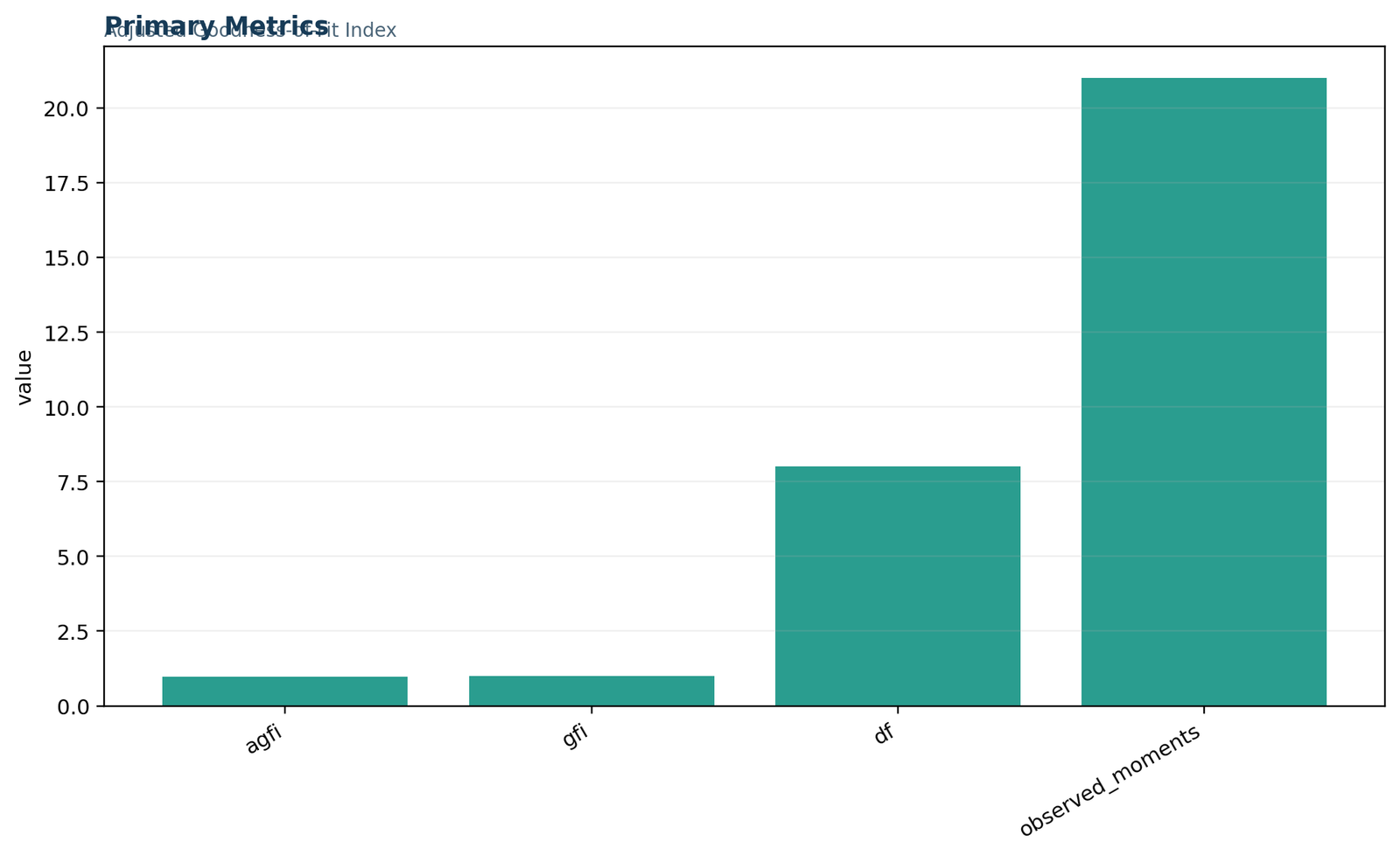
AGFI primary metrics
The primary-metrics figure summarizes the cross-software result set: AGFI = 0.980667, GFI = 0.992635, df = 8 and 21 covariance moments. The chart is a compact reproducibility check. It should not be interpreted as if df and the two fit indices share a common substantive scale.
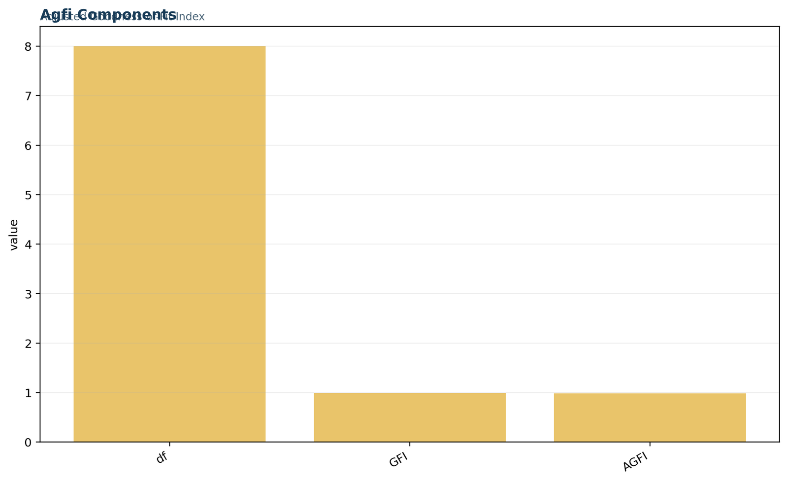
Components behind AGFI
The second chart makes the parsimony correction explicit. With six indicators, the covariance matrix contains 21 nonredundant moments. Dividing 21 by eight model degrees of freedom gives a penalty multiplier of 2.625, so AGFI is necessarily lower than GFI for this overidentified model.
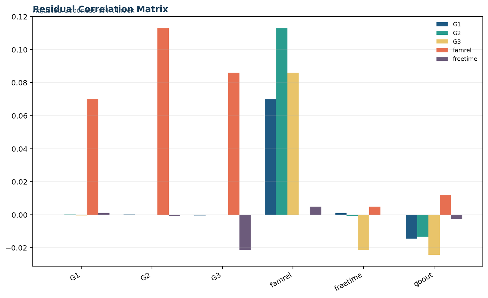
Residual correlation matrix
The residual-correlation chart shows that the strongest remaining local discrepancies connect academic grades with famrel. A high AGFI does not erase these residuals. The correct workflow therefore combines the fit-index table with residual inspection and substantive review of cross-factor covariances.
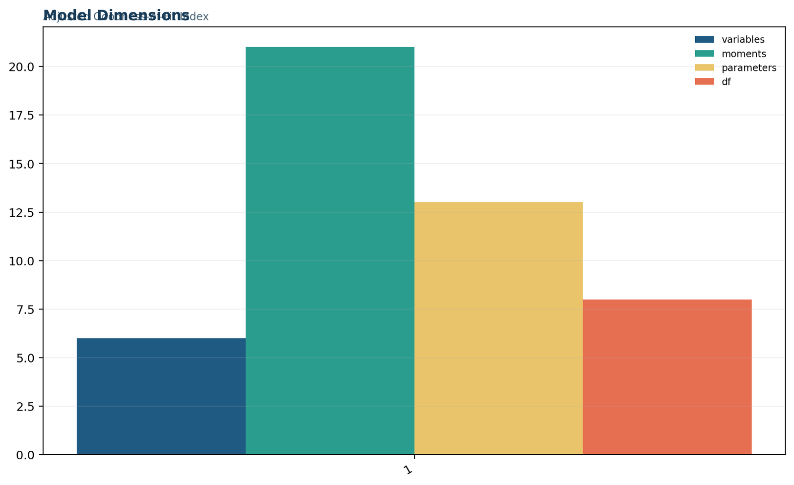
Model dimensions
This chart is an identification ledger: p = 6, = 21, free parameters = 13 and df = 8. It is especially useful when a modified CFA model unexpectedly changes AGFI, because any added loading, residual covariance or equality constraint can change the parameter count and therefore the adjustment.
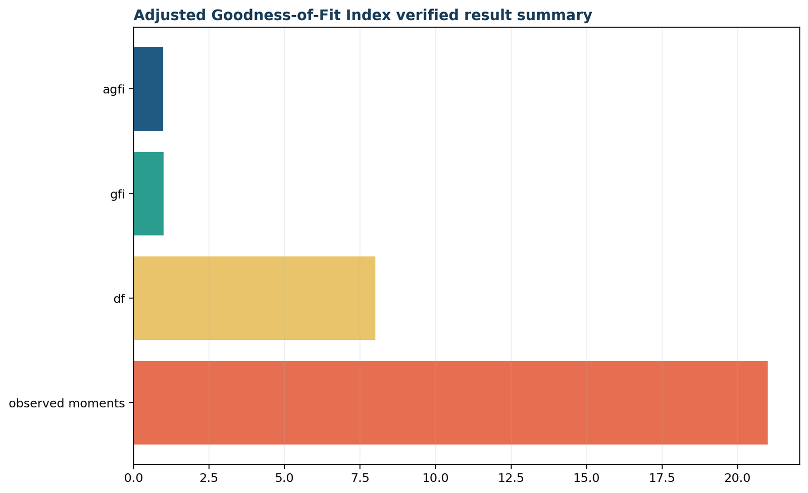
Verified result summary
The verification chart demonstrates that the reported value is not a copied cutoff judgment. It is linked to the fitted model, GFI, degrees of freedom, moment count and residual matrix. Round only in the narrative; retain the full numeric result in the analysis object and PDF.
AGFI versus GFI, CFI, TLI, RMSEA and SRMR
No single index can replace a complete global and local model-fit assessment.
| Index | Fit family | Direction of better fit | What it adds beyond AGFI | Reporting caution |
|---|---|---|---|---|
| GFI | Absolute fit | Closer to 1 | Unadjusted covariance-reproduction summary | Can favor more complex models |
| AGFI | Adjusted absolute fit | Generally closer to 1 | Penalizes GFI shortfall using df | Historical cutoffs are not universal |
| CFI | Incremental fit | Closer to 1 | Compares target model with baseline model | Depends on baseline-model misfit |
| TLI | Incremental/parsimony | Closer to 1 | Stronger complexity sensitivity than CFI | Can exceed conventional bounds |
| RMSEA | Approximate fit | Closer to 0 | Includes df and supports interval estimates | Unstable in very low-df models |
| SRMR | Standardized residual fit | Closer to 0 | Directly summarizes standardized residual size | Averages can hide particular large residuals |
AGFI and GFI should not be confused with the categorical Chi square goodness of fit test despite the shared phrase “goodness of fit.” The chi-square goodness-of-fit test compares observed frequencies with expected frequencies, whereas AGFI evaluates a fitted covariance model.
How to report AGFI, troubleshoot disagreements and state limitations
Use exact model details, a rounded fit profile, local diagnostics and reproducibility information.
Recommended reporting sentence
“A two-factor confirmatory factor analysis was estimated in R for 649 observations. The Academic factor was measured by G1, G2 and G3, and the Social factor by famrel, freetime and goout. The model showed strong adjusted global fit, GFI = .993 and AGFI = .981, with 8 degrees of freedom. Residual-correlation inspection identified the largest local discrepancy between G2 and famrel (residual = .113), so global fit was interpreted alongside local diagnostics.”
Minimum technical details
Claims to avoid
Cross-software troubleshooting checklist
R and lavaan
Python and semopy
SPSS Statistics and Amos
Excel workbook
Limitations that belong in the final interpretation
Global averaging
AGFI compresses many covariance discrepancies into one value. A high result can coexist with a meaningful local residual.
Cutoff dependence
The historical .90 guideline is not a universal law. Model size, degrees of freedom, estimator and data quality matter.
Reliability separation
Good global fit does not prove reliable measurement. The weak social-indicator consistency in this example remains important.
Model equivalence
Different structural models can reproduce the same or very similar covariance patterns.
Sample dependence
AGFI describes the analyzed sample. Replication or cross-validation is needed before generalizing the model.
Causal limits
A high CFA fit index does not establish causal direction among latent variables or indicators.
AGFI PDF, SPSS output and worked Excel downloads
Use the software reports and workbook together for a complete cross-check.
Adjusted Goodness of Fit Index frequently asked questions
Direct answers about the formula, interpretation and four software workflows.
What is the Adjusted Goodness of Fit Index?
AGFI is a model-fit index derived from GFI with an adjustment for the degrees of freedom available to test a covariance-structure model. It summarizes global covariance reproduction with a complexity penalty.
Is AGFI a statistical test?
No. AGFI is a descriptive fit index. It does not have the same interpretation as a p-value and should not be reported as if a null hypothesis were directly accepted or rejected by the index.
What is a good AGFI value?
Larger values generally indicate better global fit, and .90 is often used as a historical rule of thumb. A fixed cutoff is not a universal law. Estimator, model size, indicator quality, residuals and the complete fit profile must be considered.
Can AGFI be higher than GFI?
Under the conventional positive-df adjustment, AGFI is usually less than or equal to GFI because the GFI shortfall is multiplied by a factor related to complexity. Unusual implementations or pathological models require formula verification.
Why does AGFI decrease when paths are added?
Adding free parameters reduces degrees of freedom. Even if raw fit improves, the parsimony adjustment can offset part of that improvement.
Can AGFI be negative?
Yes, some formulations can produce negative values for very poor-fitting or low-df models. Do not truncate the value silently; investigate model specification and the software definition.
Should AGFI be reported alone?
No. Report it with the model chi-square and df plus complementary indices such as CFI, TLI, RMSEA and SRMR, and include local residual or parameter diagnostics.
Does a high AGFI prove the model is correct?
No. Many different models can reproduce a covariance matrix well. Fit is necessary evidence for a proposed model, not proof of causal truth, construct validity or unique specification.
What does df = 8 mean here?
Six observed variables provide 21 unique covariance moments. The model estimates 13 free parameters, leaving 21 − 13 = 8 degrees of freedom for evaluating global fit.
Why are G1, G2 and G3 grouped together?
They are repeated academic performance measures with strong correlations in the supplied data. The model treats them as indicators of an Academic latent factor.
Why inspect the residual correlation matrix?
A global index can look excellent while specific indicator pairs remain under- or over-reproduced. Residuals locate those local discrepancies.
How do I obtain AGFI in R?
Fit the CFA with lavaan and request df, GFI and AGFI from the fitted object with the fit-index table. Preserve the exact model syntax and estimator.
How do I obtain AGFI in Python?
Fit the CFA with semopy, run calc_stats(model), and read DoF, GFI and AGFI from the returned fit table. Verify the result independently with full-precision values.
Where is AGFI in SPSS?
AGFI is associated with IBM SPSS Amos rather than the standard SPSS Statistics FACTOR command. In Amos, inspect the model-fit output containing RMR, GFI, AGFI and PGFI when available.
Can Excel calculate AGFI?
Yes, Excel can reproduce AGFI when p, free parameters or model df, and a valid GFI from a fitted covariance model are supplied. Excel does not replace the SEM estimator that produced GFI.