
Hierarchical Regression: Formula, Interpretation, SPSS, Python, R and Excel Guide
Hierarchical Regression tests whether theoretically ordered predictor blocks explain additional variance beyond variables already entered. This worked analysis predicts final grade G3 for 649 students, compares three nested models, interprets the R² changes, and connects each block decision to coefficients, diagnostics and prediction error.
3 predictor blocks
28 final predictors
Python · R · SPSS · Excel
Model Overview
What this model is and when it is used: Hierarchical Regression is a planned form of multiple linear regression in which predictors are entered in researcher-defined blocks based on theory, timing, control needs or incremental-validity questions. It is used when the dependent variable is continuous and the analyst wants to determine whether a later set of variables explains additional outcome variance after earlier controls have already entered. Predictors may be continuous, ordinal, binary or categorical, with categorical variables represented through indicator coding. Every later model must contain all earlier predictors, use the same observations and retain the same coding so that changes in R² and nested F tests have a valid interpretation.
Quick Answer
Block 2 is the decisive improvement
G1, G2, studytime, failures and absences add 72.97 percentage points of explained variance beyond demographics.
- F-change(5, 637) = 629.7720
- p < .001
- RMSE falls from 3.0237 to 1.2403
- MAE falls from 2.2508 to 0.7794
Block 3 adds complexity, not meaningful fit
Seventeen family, support and behavioral terms raise raw R² only from 0.8524 to 0.8563.
- F-change(17, 620) = 0.9902
- p = .4674
- Adjusted R² remains 0.8498
- AIC and BIC both worsen
Table of Contents
- Why hierarchical regression is needed
- How the block sequence works
- Variables and coding
- Results at a glance
- Detailed block-by-block interpretation
- Python chart stories
- R charts with explanation boxes
- Final coefficients
- Diagnostics and model choice
- SPSS, Python, R and Excel
- Code
- Advanced interpretation
- APA-style reporting
- Publication checklist
- Downloads
- Related guides
- FAQs
Why Use Hierarchical Regression?
Hierarchical Regression is appropriate when the scientific question is conditional. Instead of asking only whether a final collection of predictors explains G3, the analysis asks whether academic variables add information beyond demographics and whether family, support and behavioral variables add anything after prior achievement is already known.
The order assigns shared variance to the block that enters first. Therefore, block order must be justified before inspecting the results. In this analysis, demographics are controls, prior grades are the central incremental block, and the broad family/support/behavior block is tested last.
How the Three-Block Model Works
Age and demographic contrasts establish the baseline explanation.
G1, G2, studytime, failures and absences test incremental achievement information.
Seventeen additional terms test whether broader context adds beyond Blocks 1–2.
The nested F-change test evaluates the joint null hypothesis that every newly added slope equals zero. The test is valid only when the models are genuinely nested and use the same 649 observations.
Hierarchical Regression is not a multilevel model. The hierarchy describes predictor entry, not students nested within schools. No random intercept, random slope, variance component or intraclass correlation coefficient is estimated.
Variables Used and Coding
| Variable(s) | Block | Meaning and coding | Type |
|---|---|---|---|
| G3 | Outcome | Final grade measured from 0 to 19. | Continuous dependent variable |
| age | Block 1 | Student age in years. | Numeric predictor |
| school_MS | Block 1 | MS school; GP is reference. | Binary indicator |
| sex_M | Block 1 | Male; female is reference. | Binary indicator |
| address_U | Block 1 | Urban; rural is reference. | Binary indicator |
| famsize_LE3 | Block 1 | Family size ≤3; GT3 is reference. | Binary indicator |
| Pstatus_T | Block 1 | Parents together; apart is reference. | Binary indicator |
| G1 | Block 2 | First-period grade. | Numeric predictor |
| G2 | Block 2 | Second-period grade. | Numeric predictor |
| studytime | Block 2 | Weekly study-time category. | Ordinal predictor |
| failures | Block 2 | Previous class failures. | Count/ordinal predictor |
| absences | Block 2 | School absence count. | Count predictor |
| Medu, Fedu | Block 3 | Mother’s and father’s education. | Ordinal predictors |
| traveltime | Block 3 | Travel-time category. | Ordinal predictor |
| famrel, freetime, goout | Block 3 | Family relationship, free time and social activity. | Ordinal predictors |
| Dalc, Walc | Block 3 | Workday and weekend alcohol-use categories. | Ordinal predictors |
| health | Block 3 | Self-rated health category. | Ordinal predictor |
| schoolsup, famsup, paid | Block 3 | School, family and paid-class support. | Binary indicators |
| activities, nursery, higher | Block 3 | Activities, nursery attendance and higher-education intention. | Binary indicators |
| internet, romantic | Block 3 | Internet access and romantic relationship. | Binary indicators |
Results at a Glance
F(6,642)=14.9603, p<.001
F-change=629.7720, p<.001
F-change=0.9902, p=.4674
Adjusted R² = 0.8498
MAE = 0.7700
Lowest AIC and BIC
| Model | Predictors | R² | Adjusted R² | ΔR² | Overall F | F-change | Change p | RMSE | MAE | AIC | BIC |
|---|---|---|---|---|---|---|---|---|---|---|---|
| Block 1 | 6 | 0.1227 | 0.1145 | 0.1227 | 14.9603 | Initial model | <.001 | 3.0237 | 2.2508 | 3291.9944 | 3323.3224 |
| Block 2 | 11 | 0.8524 | 0.8498 | 0.7297 | 334.3804 | 629.7720 | <.001 | 1.2403 | 0.7794 | 2145.3085 | 2199.0137 |
| Block 3 | 28 | 0.8563 | 0.8498 | 0.0039 | 131.9304 | 0.9902 | .4674 | 1.2238 | 0.7700 | 2161.9234 | 2291.7109 |
Download the PDF Outputs
The same reports are available again in the complete Downloads section near the end.
Detailed Block-by-Block Interpretation
Block 1: Background and Demographic Controls
Block 1 establishes the baseline regression using age, school, sex, address, family size and parental living status. Together, these six terms explain 12.27% of the observed variance in final grade G3, with R² = 0.1227 and adjusted R² = 0.1145. The model is statistically significant, F(6, 642) = 14.9603, p < .001, which means the demographic block performs better than an intercept-only model when the six slopes are tested jointly.
Despite statistical significance, Block 1 has limited fitted accuracy. Its RMSE is 3.0237 and its MAE is 2.2508. On average, predictions based only on background variables miss the observed final grade by more than two points in absolute terms. This establishes an important practical baseline: demographics contain relevant information, but they are not sufficient for accurate final-grade prediction.
The Block 1 AIC of 3291.9944 and BIC of 3323.3224 are much larger than those of later models. The sharp improvement after academic variables enter shows that the baseline model leaves a large amount of systematic grade variation unexplained.
Block 2: Prior Achievement and Academic Variables
Block 2 retains every Block 1 predictor and adds G1, G2, studytime, failures and absences. The model R² rises from 0.1227 to 0.8524, producing an incremental ΔR² = 0.7297. Thus, the five newly entered academic variables jointly explain an additional 72.97 percentage points of G3 variance after demographic controls have already been considered.
The improvement is statistically decisive: F-change(5, 637) = 629.7720, p < .001. This test evaluates the joint null hypothesis that the five new slopes are all zero after controlling for Block 1. The observed F-change is extremely large, so the null hypothesis is rejected.
Block 2 also transforms fitted accuracy. RMSE falls from 3.0237 to 1.2403, a reduction of 1.7834 grade points. MAE falls from 2.2508 to 0.7794, a reduction of 1.4714 grade points. These reductions confirm that the R² increase reflects a major practical improvement, not merely a statistically significant change in a large sample.
Adjusted R² reaches 0.8498, only 0.0026 below raw R². The small penalty indicates that the five added terms contribute far more explanatory value than would be expected from model expansion alone. Block 2 also has the lowest AIC = 2145.3085 and BIC = 2199.0137, making it the preferred balance of fit and complexity.
Block 3: Family, Support and Behavioral Variables
Block 3 adds seventeen parental-education, family, support, health, activity, internet, alcohol-use and relationship terms. Raw R² increases from 0.8524 to 0.8563, so the complete block adds only ΔR² = 0.0039, or 0.39 percentage points.
The corresponding test is not significant, F-change(17, 620) = 0.9902, p = .4674. Therefore, the seventeen new slopes do not jointly reduce residual error enough to demonstrate incremental explanatory value after the demographic and academic blocks are already in the model.
Adjusted R² remains 0.8498, showing that the small raw R² increase is offset by the penalty for seventeen additional terms. AIC rises from 2145.3085 to 2161.9234, while BIC rises from 2199.0137 to 2291.7109. The BIC increase of 92.6972 is especially strong evidence against the larger specification when parsimony is important.
Block 3 slightly lowers fitted RMSE from 1.2403 to 1.2238 and MAE from 0.7794 to 0.7700. These reductions are only 0.0165 and 0.0094 respectively. Because ordinary least squares cannot worsen the training residual sum of squares when predictors are added, tiny fitted-error reductions are expected even when the added variables do not generalize.
Overall Model Decision
The complete 28-predictor model is statistically significant, F(28, 620) = 131.9304, p < .001, and explains 85.63% of the observed G3 variance. However, the final-model test answers whether all 28 slopes are jointly zero. It does not answer whether the final seventeen-variable block adds information beyond Blocks 1 and 2.
The correct decision is therefore two-part. The complete model may be reported because it represents the pre-specified analysis, but Block 2 is the preferred parsimonious model because it has the same adjusted R², lower AIC, lower BIC and a highly significant incremental contribution. Block 3 should be described as non-significant and practically small.
Python Chart Stories: What Each Figure Actually Means
Each Python figure is interpreted through four boxes: what it shows, exact values, statistical meaning and the next diagnostic step.
Python Chart 1: Outcome Distribution for G3
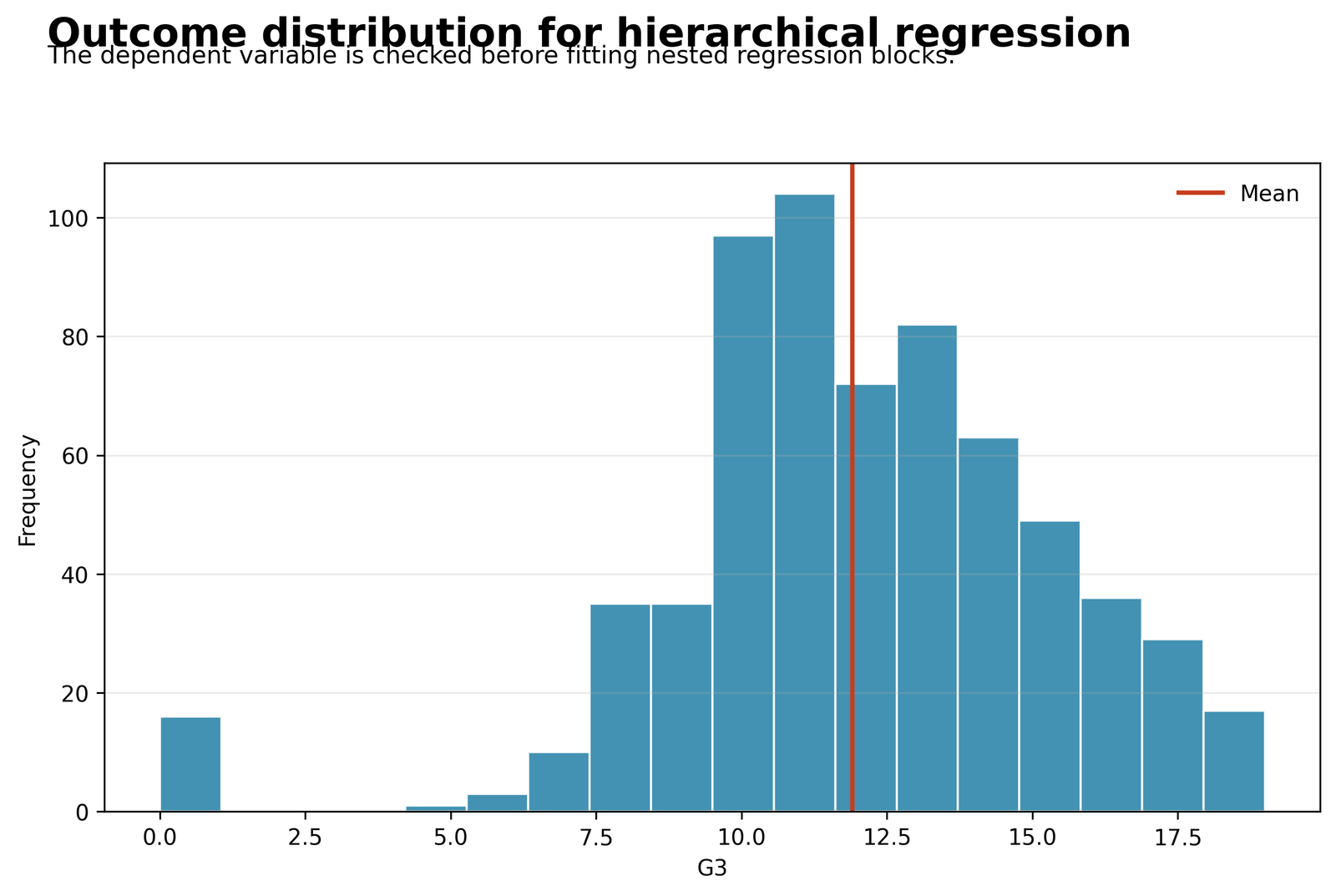
The histogram establishes the outcome scale used in every hierarchical block and shows where most final grades are concentrated.
The analysis contains 649 students. G3 has mean 11.906, SD 3.231, and range 0–19. Approximately 16 students have G3 = 0, while the tallest central bar contains just over 100 observations near grade 11.
The middle of the distribution is dense, but the small zero-grade group creates a long lower tail. Those cases later produce the largest negative residuals because prior grades predict substantially higher final outcomes.
Check residual normality, studentized residuals and influence rather than judging the regression only from the raw outcome histogram.
The distribution also helps explain why residual checks are necessary even when the overall model fit is high. G3 is integer-valued and bounded, so fitted values are continuous while observed values occur in horizontal grade bands. The relatively small group at G3 = 0 creates observations that are difficult for an ordinary linear model to predict from prior grades and background variables. These cases should be examined for data quality, unusual academic trajectories and influence, but they should not be removed solely because they reduce normality.
Python Chart 2: R² and Adjusted R² by Block
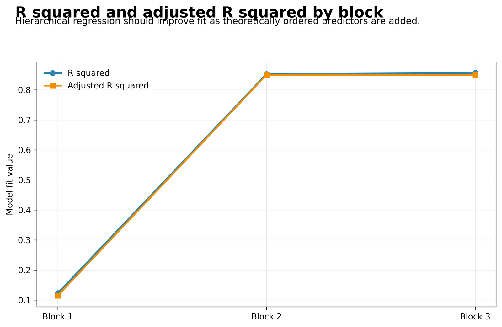
The two lines compare total explained variance with the complexity-adjusted estimate as predictors are added in theoretically ordered blocks.
Block 1 has R² = 0.1227 and adjusted R² = 0.1145. Block 2 rises to R² = 0.8524 and adjusted R² = 0.8498. Block 3 reaches R² = 0.8563, but adjusted R² remains 0.8498.
The five academic variables in Block 2 create a genuine and very large improvement. Seventeen additional Block 3 terms increase raw R² by only 0.0039 and do not improve adjusted R².
Interpret Block 3 with its F-change, AIC and BIC rather than selecting it merely because raw R² is highest.
The gap between raw and adjusted R² provides a direct complexity check. In Block 1 the gap is 0.0082. In Block 2 it falls to 0.0026 because the five new predictors contribute substantial information. In Block 3 raw R² rises by 0.0039, yet adjusted R² does not increase at the reported precision. This pattern shows why the largest raw R² should not be used automatically to choose the final specification.
Python Chart 3: Incremental R² Change
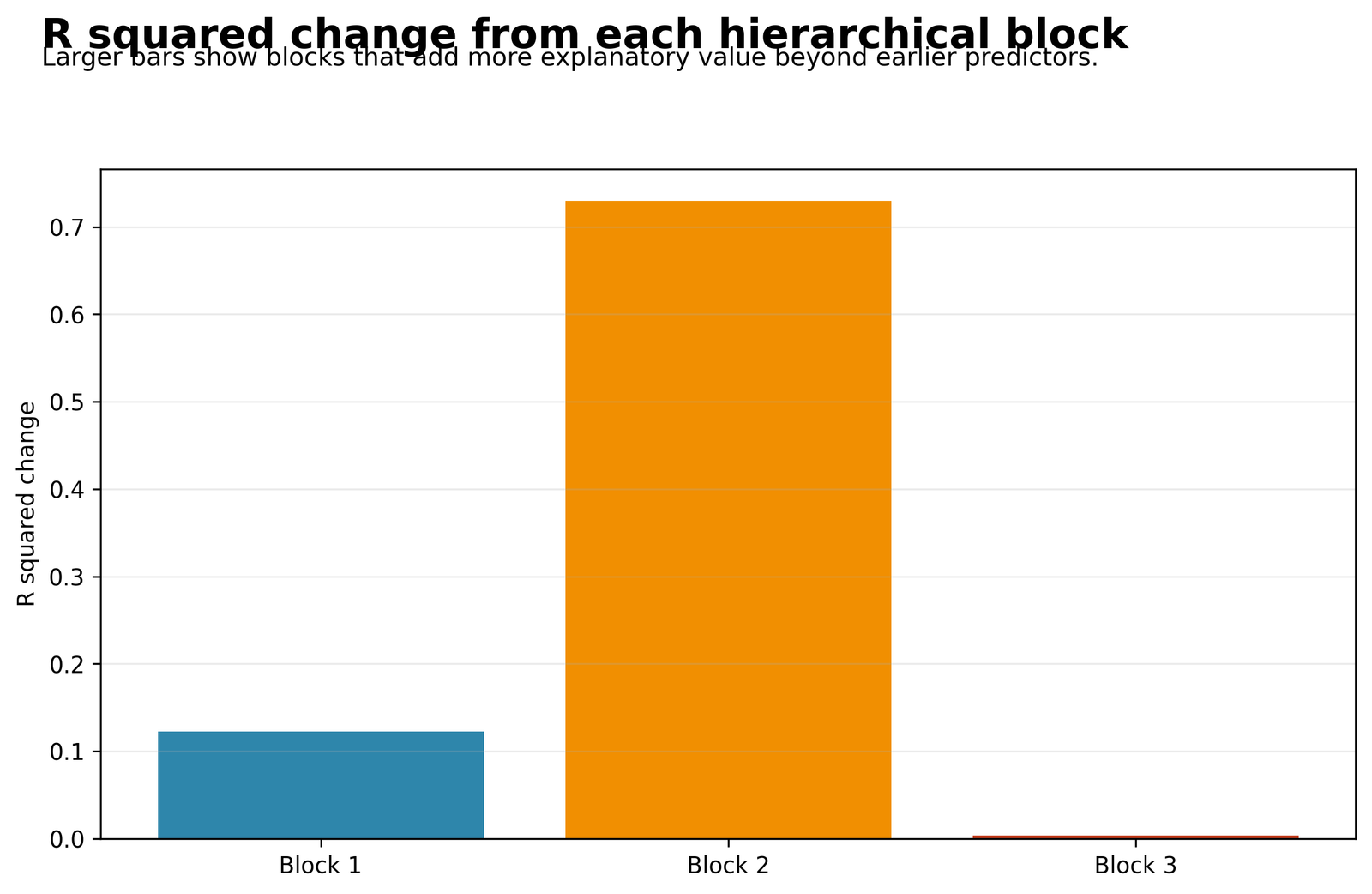
This is the central hierarchical-regression figure because it isolates what each new block contributes after all earlier variables have already entered.
Block 1 explains ΔR² = 0.1227. Block 2 adds ΔR² = 0.7297, F-change(5, 637) = 629.7720, p < .001. Block 3 adds only ΔR² = 0.0039, F-change(17, 620) = 0.9902, p = .4674.
Prior achievement and academic variables add 72.97 percentage points of explained variance beyond demographics. The family, support and behavioral block does not add statistically meaningful incremental information.
Report the scientific rationale for the block order and avoid redistributing Block 2’s joint contribution to one predictor alone.
The Block 2 bar represents the joint contribution of all five newly entered academic terms. It cannot be attributed entirely to G2, even though G2 is the strongest final predictor. G1, G2, studytime, failures and absences share explanatory variance, and the block test evaluates them as a set. The Block 3 bar similarly represents the combined contribution of seventeen terms, not seventeen separate conclusions.
Python Chart 4: Observed G3 vs Final-Model Fitted Values
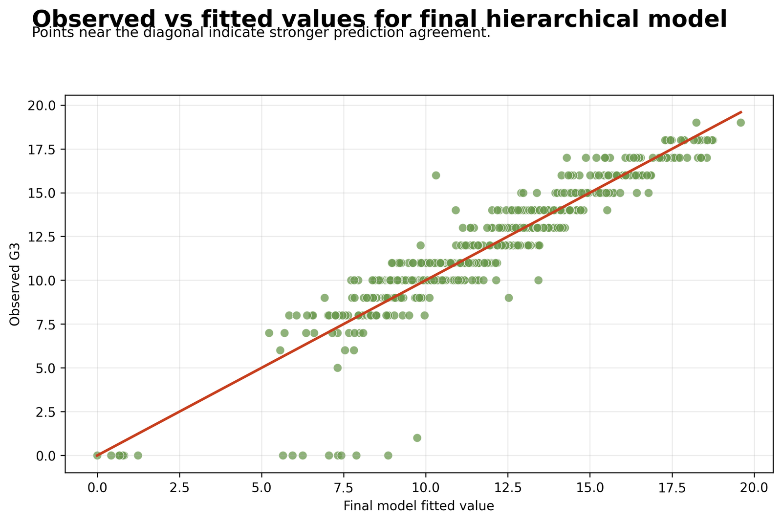
The scatterplot shows how closely final-model predictions follow the observed grade scale and identifies observations with unusually large prediction errors.
The final model has R² = 0.8563, adjusted R² = 0.8498, RMSE = 1.2238, and MAE = 0.7700. Most points follow the agreement line from fitted values near 6 to 19.
Average fitted accuracy is strong, but several students with observed G3 = 0 receive predictions between roughly 5.5 and 10. A high R² therefore does not imply uniformly accurate individual predictions.
Review the largest errors, calculate influence statistics and evaluate out-of-sample prediction before presenting the model as a forecasting tool.
The diagonal pattern is strong through the central and upper grade range, but the plot also reveals regression-to-the-mean behavior at the extremes. Very low observed grades tend to receive higher predictions, while a few high observed grades receive somewhat lower predictions. These deviations affect individual prediction even though the model explains a large proportion of total variance.
R Charts: Two Charts Followed by Two Matching Explanation Boxes
Each group displays two R charts first and then two aligned explanation boxes. On mobile, every chart stacks with its correct interpretation.
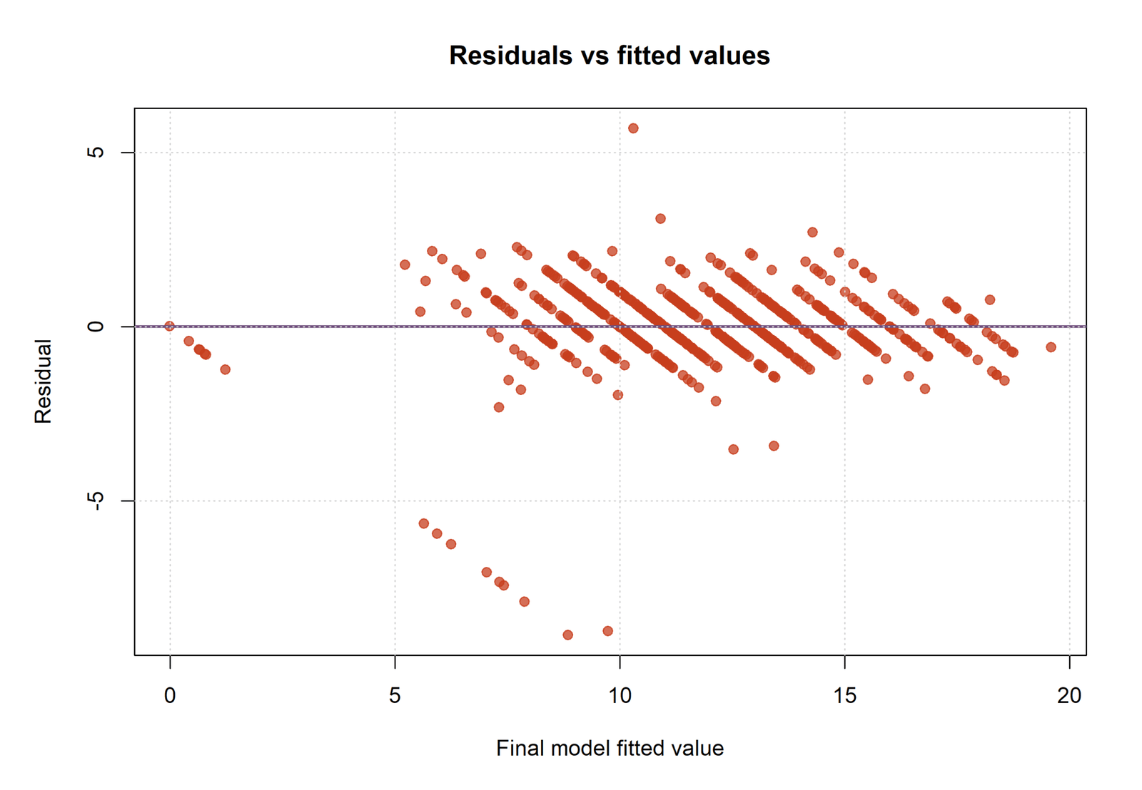
R Chart 1: Residuals vs Fitted Values
Most residuals lie between approximately -2 and +2. The largest positive residual is about +5.7, while the most negative residuals reach approximately -9.1.
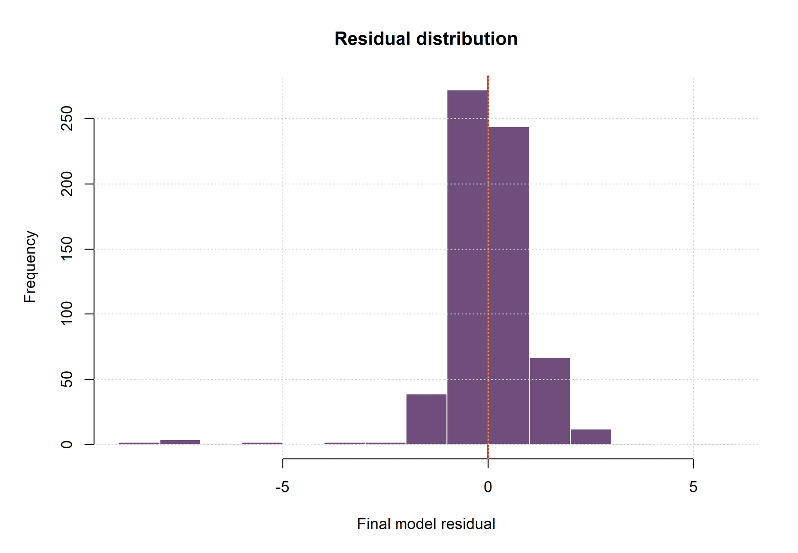
R Chart 2: Residual Distribution
The central residual mass lies near zero, with the largest bins containing approximately 244 and 210 observations. The right tail reaches about +5.7, while the left tail reaches about -9.1.
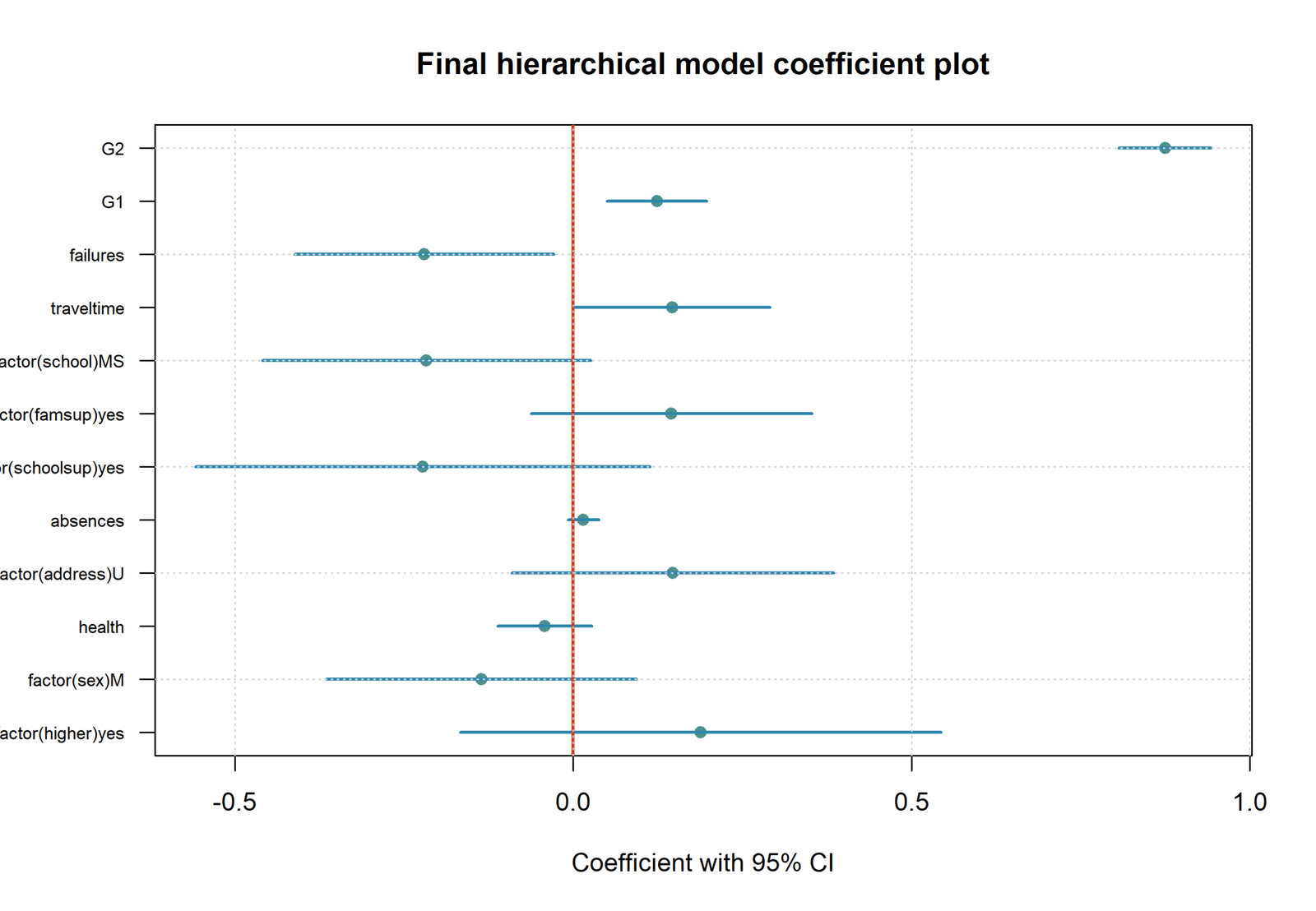
R Chart 3: Final Coefficients with 95% Confidence Intervals
G2 B = 0.8749, 95% CI [0.8064, 0.9433]; G1 B = 0.1236, CI [0.0500, 0.1972]; and failures B = -0.2206, CI [-0.4120, -0.0291].
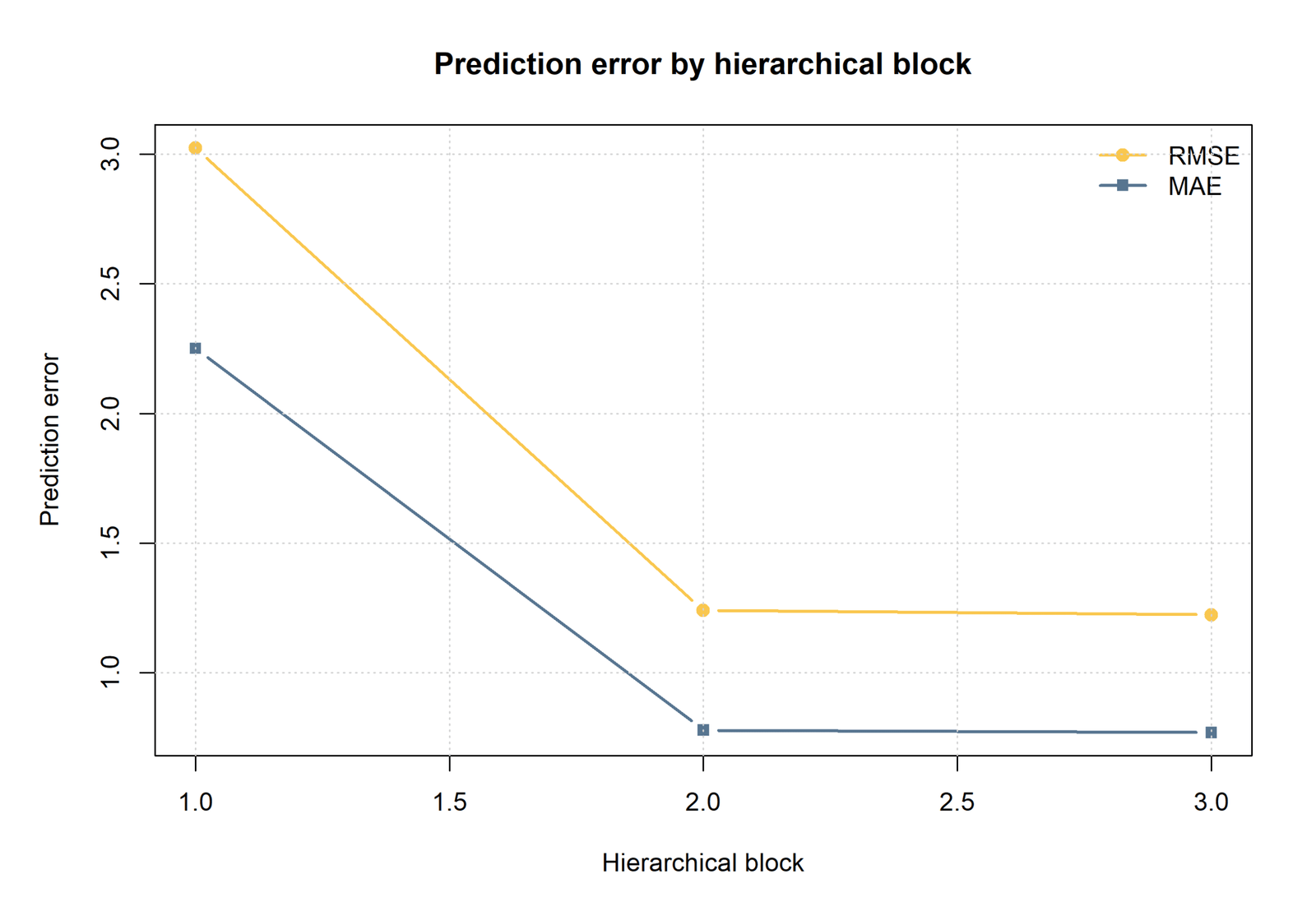
R Chart 4: RMSE and MAE by Block
RMSE declines from 3.0237 to 1.2403 and then 1.2238. MAE declines from 2.2508 to 0.7794 and then 0.7700.
Final Hierarchical-Regression Coefficients
The coefficient table describes conditional relationships in the complete 28-predictor model. It is separate from the block-level ΔR² tests. A predictor can be non-significant individually while belonging to a block that is important jointly, and a significant final coefficient does not prove that its entire block adds significant variance.
| Term | B | SE | t | p | 95% CI |
|---|---|---|---|---|---|
| Intercept | -0.0704 | 0.9220 | -0.0763 | .9392 | [-1.8809, 1.7402] |
| age | 0.0399 | 0.0464 | 0.8608 | .3897 | [-0.0512, 0.1311] |
| school_MS | -0.2171 | 0.1237 | -1.7553 | .0797 | [-0.4600, 0.0258] |
| sex_M | -0.1360 | 0.1168 | -1.1647 | .2446 | [-0.3653, 0.0933] |
| address_U | 0.1469 | 0.1211 | 1.2130 | .2256 | [-0.0909, 0.3847] |
| famsize_LE3 | 0.0496 | 0.1143 | 0.4341 | .6643 | [-0.1749, 0.2741] |
| Pstatus_T | -0.1076 | 0.1593 | -0.6750 | .4999 | [-0.4205, 0.2054] |
| G1 | 0.1236 | 0.0375 | 3.2988 | .0010 | [0.0500, 0.1972] |
| G2 | 0.8749 | 0.0349 | 25.1010 | <.001 | [0.8064, 0.9433] |
| studytime | 0.0436 | 0.0651 | 0.6700 | .5031 | [-0.0843, 0.1715] |
| failures | -0.2206 | 0.0975 | -2.2628 | .0240 | [-0.4120, -0.0291] |
| absences | 0.0148 | 0.0116 | 1.2808 | .2007 | [-0.0079, 0.0376] |
| Medu | -0.0520 | 0.0612 | -0.8489 | .3963 | [-0.1722, 0.0683] |
| Fedu | 0.0311 | 0.0599 | 0.5183 | .6045 | [-0.0866, 0.1487] |
Strongest positive predictor
G2 B = 0.8749. Holding all 27 other predictors constant, one additional G2 point is associated with approximately 0.875 additional G3 points.
Significant negative predictor
failures B = -0.2206. One additional previous failure is associated with about 0.221 fewer G3 points after adjustment.
Diagnostics and Model Choice
Why Block 2 is preferred
- Adjusted R² = 0.8498
- AIC = 2145.3085
- BIC = 2199.0137
- F-change p < .001
- Large fitted-error reduction
Why Block 3 is not preferred
- Adjusted R² remains 0.8498
- AIC rises by 16.6149
- BIC rises by 92.6972
- F-change p = .4674
- RMSE falls by only 0.0165
SPSS, Python, R and Excel Workflows
Python
Fit three nested statsmodels OLS equations and compare consecutive models with compare_f_test().
- Same 649 rows in every model
- Exact dummy references
- R², adjusted R², AIC, BIC, RMSE and MAE
R
Fit nested lm() models and use anova(m1,m2,m3) for sequential F tests.
- Factor references must match
- Use identical complete cases
- Validate coefficient and chart values
SPSS
Use Linear Regression with successive ENTER blocks and request R Square Change, ANOVA, confidence intervals and collinearity diagnostics.
- Block 1 demographics
- Block 2 academic variables
- Block 3 family/support/behavior
Excel
Run separate regressions for each block using the same rows, then calculate ΔR² and F-change from the model summaries.
=R2_New-R2_Previous=F.DIST.RT(Fchange,df1,df2)- Compare adjusted R² and residual error
Code: Expand Only the Software You Need
Python nested OLS code
import pandas as pd
import statsmodels.formula.api as smf

df = pd.read_csv("dataset.csv")

block1 = (
    "G3 ~ age + C(school) + C(sex) + C(address)"
    " + C(famsize) + C(Pstatus)"
)
block2 = (
    block1 + " + G1 + G2 + studytime + failures + absences"
)
block3 = (
    block2
    + " + Medu + Fedu + traveltime + famrel + freetime"
    + " + goout + Dalc + Walc + health"
    + " + C(schoolsup) + C(famsup) + C(paid)"
    + " + C(activities) + C(nursery) + C(higher)"
    + " + C(internet) + C(romantic)"
)

required = sorted(set(
    ["G3", "age", "school", "sex", "address", "famsize", "Pstatus",
     "G1", "G2", "studytime", "failures", "absences", "Medu", "Fedu",
     "traveltime", "famrel", "freetime", "goout", "Dalc", "Walc",
     "health", "schoolsup", "famsup", "paid", "activities", "nursery",
     "higher", "internet", "romantic"]
))
work = df[required].dropna().copy()

m1 = smf.ols(block1, data=work).fit()
m2 = smf.ols(block2, data=work).fit()
m3 = smf.ols(block3, data=work).fit()

f12, p12, df12 = m2.compare_f_test(m1)
f23, p23, df23 = m3.compare_f_test(m2)

print(m1.summary())
print(m2.summary())
print(m3.summary())
print("Block 2 change:", f12, p12, df12)
print("Block 3 change:", f23, p23, df23)
R nested lm code
df <- read.csv("dataset.csv", stringsAsFactors = TRUE)

vars <- c(
  "G3","age","school","sex","address","famsize","Pstatus",
  "G1","G2","studytime","failures","absences","Medu","Fedu",
  "traveltime","famrel","freetime","goout","Dalc","Walc",
  "health","schoolsup","famsup","paid","activities","nursery",
  "higher","internet","romantic"
)
work <- na.omit(df[vars])

m1 <- lm(
  G3 ~ age + school + sex + address + famsize + Pstatus,
  data = work
)
m2 <- update(
  m1, . ~ . + G1 + G2 + studytime + failures + absences
)
m3 <- update(
  m2, . ~ . + Medu + Fedu + traveltime + famrel +
    freetime + goout + Dalc + Walc + health + schoolsup +
    famsup + paid + activities + nursery + higher +
    internet + romantic
)

anova(m1, m2, m3)
summary(m1)
summary(m2)
summary(m3)
AIC(m1, m2, m3)
BIC(m1, m2, m3)
SPSS sequential ENTER syntax
REGRESSION
 /DEPENDENT G3
 /METHOD=ENTER age school_MS sex_M address_U famsize_LE3 Pstatus_T
 /METHOD=ENTER G1 G2 studytime failures absences
 /METHOD=ENTER Medu Fedu traveltime famrel freetime goout
   Dalc Walc health schoolsup_yes famsup_yes paid_yes
   activities_yes nursery_yes higher_yes internet_yes romantic_yes
 /STATISTICS COEFF OUTS R ANOVA CHANGE CI(95) COLLIN TOL
 /RESIDUALS HISTOGRAM(ZRESID) NORMPROB(ZRESID)
 /CASEWISE PLOT(ZRESID) OUTLIERS(3)
 /SAVE PRED RESID ZPRED ZRESID COOK LEVER.

OUTPUT SAVE
 /OUTFILE='D:\DATA ANALYSIS\H Regression Tests and Models\Hierarchical Regression\SPSS_Output\spv\Hierarchical-Regression.spv'.

OUTPUT EXPORT
 /CONTENTS EXPORT=ALL LAYERS=PRINTSETTING MODELVIEWS=PRINTSETTING
 /PDF DOCUMENTFILE='D:\DATA ANALYSIS\H Regression Tests and Models\Hierarchical Regression\SPSS_Output\pdf\Hierarchical-Regression-SPSS-Output.pdf'.
Excel formulas
Block 2 R-squared change:
=R2_Block2-R2_Block1

Block 3 R-squared change:
=R2_Block3-R2_Block2

F-change:
=(Delta_R2/New_Predictors)/
 ((1-R2_Full)/(N-Full_Predictors-1))

F-change p-value:
=F.DIST.RT(F_Change,New_Predictors,Residual_DF)

Adjusted R-squared:
=1-(1-R2)*(N-1)/(N-Predictors-1)

RMSE:
=SQRT(AVERAGE(Squared_Residual_Range))

MAE:
=AVERAGE(Absolute_Residual_Range)
Advanced Interpretation and Extensions
The main reading path remains compact. Expand only the technical topics needed for the study.
Joint significance versus individual significance
A block can be significant even when not every individual coefficient is significant because the nested F test evaluates all newly added slopes together. Conversely, one coefficient may be significant in a large block even when the block-level F-change is not significant.
In this analysis, the central scientific conclusion comes from both levels: Block 2 is jointly significant, and G1, G2 and failures remain significant in the final specification. Block 3 is not jointly significant, even though individual estimates within that block may vary in magnitude.
Why G2 dominates the final model
G2 is the second-period grade and is temporally and conceptually close to final grade G3. Its final unstandardized coefficient is 0.8749 with a very narrow confidence interval from 0.8064 to 0.9433.
The coefficient means that, holding the other 27 predictors constant, one additional G2 point is associated with approximately 0.875 additional G3 points. The strong adjusted relationship also explains why Block 2 produces such a large increase in R².
G2’s large coefficient does not mean it alone accounts for the entire Block 2 ΔR². G1, failures, studytime and absences enter simultaneously and share predictive information with G2.
Why G1 remains significant after G2 enters
G1 is measured earlier than G2, yet it retains a positive final coefficient of 0.1236, p = .0010. This indicates that first-period achievement contributes information about G3 that is not completely captured by G2 and the other predictors.
Because G1 and G2 are correlated, their final slopes are conditional effects. The G1 coefficient should not be compared directly with its simple correlation with G3. Its interpretation is the expected G3 difference associated with one G1 point among students who are otherwise equal on G2 and all remaining model terms.
Why failures is negative after adjustment
The failures coefficient is -0.2206, with a 95% confidence interval from -0.4120 to -0.0291. Holding the other predictors constant, each additional prior failure is associated with approximately 0.221 fewer final-grade points.
The effect is smaller than the prior-grade effects, but its interval excludes zero. Because failures is a bounded count/ordinal variable, researchers should also inspect whether a linear slope adequately represents the difference between zero, one, two and three prior failures.
Why school is close to significance but not significant
The school_MS coefficient is -0.2171 with p = .0797 and a confidence interval from -0.4600 to 0.0258. The interval includes zero, so the adjusted school contrast is not statistically significant at alpha .05.
This does not prove that GP and MS have identical outcomes. It means the estimated conditional difference is not sufficiently precise after prior achievement and all other predictors are controlled. The two-school structure may also require multilevel or cluster-aware sensitivity analysis when the objective is a population-level school effect.
Why absences is positive but non-significant
The final absences coefficient is 0.0148, p = .2007, with a confidence interval from -0.0079 to 0.0376. The positive sign should not be interpreted as evidence that absences improve grades because the interval includes zero.
The adjusted sign can differ from the simple relationship because prior grades, failures, school and other variables are controlled. Nonlinearity, a concentration of zeros and influential high-absence observations may also affect the linear slope.
How to report the preferred model without hiding the planned final block
Report the complete pre-specified block sequence, including the non-significant Block 3 result. Then explain that Block 2 is preferred for parsimony because adjusted R² is unchanged, the Block 3 F-change is non-significant, and AIC and BIC increase.
Do not delete Block 3 from the report after observing its p-value. The transparent approach is to present the planned analysis, state the incremental decision and distinguish the confirmatory block test from the preferred predictive or parsimonious specification.
How to compare the models with cross-validation
Split the data or use repeated K-fold cross-validation. Within each training fold, reproduce all preprocessing, reference coding and model fitting. Generate predictions for the held-out fold and calculate RMSE, MAE and calibration for each block.
If Block 3 does not improve held-out error, the fitted-sample conclusion is strengthened. If it improves validation despite a non-significant F-change, the difference may reflect the distinction between inferential testing and predictive utility.
How block size affects the F-change test
The numerator degrees of freedom equal the number of newly added terms. Block 2 tests five slopes, while Block 3 tests seventeen. A broad block must collectively reduce residual error enough to justify every added degree of freedom.
Adding many weak or redundant terms can produce a small raw R² increase but a non-significant F-change. This is exactly what occurs in Block 3.
How to interpret the final intercept
The intercept is -0.0704 and is not significant. It represents the expected G3 value when every numeric predictor equals zero and every categorical variable is in its reference category.
Because age, G1, G2 and several ordinal predictors cannot all take substantively realistic zero values for a typical student, the intercept has little practical meaning. Centering selected continuous predictors can create a more interpretable reference profile without changing fitted values or R².
Why R-squared change depends on order
When predictors share explanatory variance, the block entered first receives credit for the shared portion. A later block is tested only against the outcome variance that remains after earlier blocks have been fitted.
Therefore, ΔR² is not an order-free property of a variable set. The reported 0.7297 for Block 2 means academic variables add that amount after demographics; it does not mean they would add the same amount if entered after every family and behavioral variable.
How semi-partial correlation relates to incremental variance
When one predictor enters by itself, its squared semi-partial correlation equals the change in R² attributable uniquely to that predictor after earlier terms are removed from the predictor.
For a multi-predictor block, ΔR² represents the joint semi-partial contribution of the entire block. The 0.7297 Block 2 contribution cannot be assigned entirely to G2 even though G2 has the largest final coefficient.
How to interpret a non-significant block
A non-significant F-change means the new coefficients do not jointly reduce residual error enough to reject the null hypothesis under the model assumptions.
It does not prove that every variable is unrelated to the outcome in every population. A block may still be retained because it contains essential controls, but its lack of incremental evidence must be reported.
Why adjusted R-squared stays unchanged
Adjusted R² rewards explained variance but penalizes the number of predictors. Block 3 adds only 0.0039 raw R² while introducing 17 terms, so the added fit is insufficient to offset the complexity penalty.
The unchanged value of 0.8498 does not mean the models are numerically identical. It means their complexity-adjusted explanatory estimates round to the same value.
Interpreting AIC and BIC in nested regression
AIC and BIC combine likelihood-based fit with a complexity penalty. Lower values are preferred among models fitted to the same outcome and observations.
Block 2 has AIC 2145.3085 and BIC 2199.0137. Block 3 raises these to 2161.9234 and 2291.7109. The especially large BIC increase reflects its stronger penalty for 17 extra terms.
Why fitted RMSE and MAE still decline in Block 3
Ordinary least squares cannot increase the training residual sum of squares when predictors are added. Fitted RMSE and MAE may therefore decline slightly even when the added block is noise.
The Block 3 reduction is only 0.0165 RMSE and 0.0094 MAE. Validation data are needed to determine whether that tiny improvement survives outside the fitted sample.
Interpreting unstandardized and standardized coefficients
Unstandardized B values remain in the original outcome and predictor units. G2 B = 0.8749 is therefore directly interpretable in grade points.
Standardized beta coefficients can help compare predictors measured in different units, but they depend on sample variability and dummy-category prevalence. They do not replace block-level ΔR².
Reference categories and dummy coding
Every categorical coefficient compares a named category with an omitted reference. Changing the reference alters the displayed contrast and intercept but leaves fitted values, total R² and overall factor information unchanged.
Reference categories must match across Python, R and SPSS before coefficient values can be compared.
Durbin-Watson and observation order
The Durbin–Watson statistic assesses first-order residual autocorrelation in an ordered sequence. It is most relevant when rows have a meaningful time or spatial order.
For cross-sectional student data, independence should be evaluated through the sampling and clustering structure rather than relying only on one serial-correlation statistic.
Robust and bootstrap inference
Heteroskedasticity-consistent covariance estimators can protect coefficient standard errors when residual variance is not constant.
Bootstrap procedures can estimate uncertainty for coefficients and R² changes, but resampling must respect clusters or repeated structures when observations are not independent.
Hierarchical Regression vs Hierarchical Linear Modeling
- Hierarchical Regression orders predictor blocks in repeated ordinary least-squares models.
- Hierarchical Linear Modeling represents observations nested within groups and estimates random effects.
- R² change and F-change are central here; variance components and ICC belong to multilevel analysis.
Hierarchical Regression vs Stepwise Regression
- The researcher specifies hierarchical blocks before analysis.
- Stepwise algorithms add or remove individual variables using sample-based criteria.
- Theory-driven blocks are generally more defensible for confirmatory incremental hypotheses.
Choosing the Block Order
- Place established controls first when the focal question concerns added explanatory value.
- Use temporal order when earlier measurements logically precede later ones.
- Enter main effects before interaction terms and linear effects before polynomial terms.
- State the rationale before reporting results because shared variance is credited to earlier blocks.
Incremental Cohen’s f²
- Incremental f² equals ΔR² divided by one minus the full-model R².
- Block 2 f² is approximately 0.7297/(1-0.8524)=4.9438, an exceptionally large contribution.
- Block 3 f² is approximately 0.0039/(1-0.8563)=0.0271, a small contribution.
Linearity and Functional Form
- Every numeric predictor is assumed to have a linear conditional relationship with G3 unless transformed terms are included.
- G1 and G2 may show ceiling effects near the upper grade limit.
- Partial-residual plots, polynomial terms or splines can evaluate curvature.
Homoscedasticity
- The residual variance should be reasonably stable across fitted values.
- Use the residual-vs-fitted chart, Breusch–Pagan test and robust covariance sensitivity.
- A heteroskedasticity correction changes standard errors but does not repair an incorrect mean structure.
Residual Normality
- Normality is most important for small-sample confidence intervals and tests, not for the raw outcome itself.
- The final residuals are centered but show a long negative tail.
- Review Q–Q and P–P plots together with case-level diagnostics.
Multicollinearity
- G1 and G2 are strongly related, so each final coefficient represents incremental information after the other is controlled.
- Check VIF, tolerance and condition indices for every model block.
- High collinearity may leave prediction strong while making individual slopes unstable.
Influence and Leverage
- Large negative residuals do not automatically imply influential observations.
- Influence depends on residual size, leverage and effect on the fitted coefficients.
- Review studentized residuals, Cook’s distance, leverage and DFBETAs before excluding any case.
Missing Data and Comparable Samples
- All nested models must use the same rows.
- If a later block causes additional listwise deletion, ΔR² mixes predictor contribution with sample change.
- Use a common complete-case dataset or a multivariable imputation strategy that preserves block comparisons.
Cross-Validation and Prediction
- In-sample R², RMSE and MAE describe fitted performance.
- Cross-validation should repeat preprocessing within each training fold.
- A validation comparison can determine whether Block 3 improves new-case prediction despite its non-significant fitted F-change.
Interactions and Moderation
- Enter main effects before interaction products.
- The interaction block’s ΔR² tests whether moderation adds beyond the component predictors.
- Center continuous variables when it improves interpretation, but recognize that centering does not remove structural collinearity.
Polynomial Hierarchical Regression
- Enter the linear term before squared and cubic terms.
- The later polynomial block tests whether curvature improves fit beyond a straight line.
- Retain lower-order terms whenever higher-order terms remain in the model.
Model Parsimony
- Raw R² cannot decline when predictors are added.
- Adjusted R², AIC, BIC and validation error penalize unnecessary complexity.
- Block 2 is favored because Block 3 leaves adjusted R² unchanged and worsens both information criteria.
Statistical Power for R² Change
- Power depends on sample size, number of new predictors, full-model residual variance and the smallest meaningful ΔR².
- The Block 3 test evaluates 17 slopes simultaneously.
- Plan power around the block of interest rather than only the final overall F test.
Causal Interpretation
- Hierarchical entry does not make observational coefficients causal.
- Block order controls measured variables but cannot remove unmeasured confounding, measurement error or reverse causality.
- Use causal language only when the design and identification strategy support it.
Reproducibility Across Software
- Python, R and SPSS must use identical rows, reference groups, formulas and block order.
- Small differences can arise from rounding, contrast coding or robust-standard-error choices.
- Export model summaries, coefficient tables, diagnostics and exact formula definitions with every analysis.
APA-Style Reporting
Publication Checklist and Common Mistakes
Report these items
- Continuous outcome and analyzed sample size
- Theoretical rationale for block order
- Variables and reference categories in every block
- R², adjusted R² and overall F for each model
- ΔR², F-change, degrees of freedom and p-value
- Final B, SE, t, p and confidence interval
- Residual, influence and collinearity diagnostics
- Whether error values are fitted or validated
Avoid these mistakes
- Calling hierarchical regression a multilevel model
- Choosing block order after seeing the results
- Interpreting final-model significance as block significance
- Using different rows across nested models
- Preferring the largest raw R² automatically
- Ignoring adjusted R², AIC, BIC and F-change
- Reporting fitted RMSE as external prediction accuracy
- Removing non-significant controls without theoretical review
Downloads
R Hierarchical Regression ReportNested-model verification and R chart outputs.
SPSS Hierarchical Regression OutputModel summaries, ANOVA, change statistics and coefficients.
Adjusted R-Squared GuideUnderstand complexity penalties and model comparison.
Frequently Asked Questions
What is Hierarchical Regression?
It is multiple linear regression in which predictors enter in theoretically ordered blocks and every later block is tested for additional explained variance.
What type of outcome is required?
The standard method uses a continuous dependent variable suitable for linear regression. G3 is analyzed on its 0–19 numeric scale.
What predictor types can be used?
Continuous, ordinal, binary and categorical predictors can be included. Categorical variables require indicator or contrast coding.
How many blocks are used here?
Three blocks are fitted to the same 649 observations.
What is in Block 1?
Age, school, sex, address, family size and parental status.
What is in Block 2?
G1, G2, studytime, failures and absences.
What is in Block 3?
Seventeen parental-education, family, support, behavioral and lifestyle terms.
Which block adds the most variance?
Block 2 adds ΔR² = 0.7297, or 72.97 percentage points.
Is Block 3 significant?
No. F-change(17,620) = 0.9902, p = .4674.
What is the final model R squared?
The final 28-predictor model has R² = 0.8563 and adjusted R² = 0.8498.
Which predictors are significant in the final model?
G1, G2 and failures have p-values below .05 and confidence intervals that exclude zero.
Why is Block 2 preferred?
It has the lowest AIC and BIC, the same adjusted R² as Block 3, and a highly significant incremental test.
Is Hierarchical Regression a multilevel model?
No. The hierarchy concerns predictor entry. Multilevel models concern observations nested within groups.
Is it the same as stepwise regression?
No. Hierarchical blocks are selected from theory before analysis; stepwise methods use automated sample-based selection.
Can SPSS run the analysis?
Yes. Use successive METHOD=ENTER blocks and request R Square Change.
Can R run the analysis?
Yes. Fit nested lm models and compare them with anova.
Can Excel calculate F-change?
Yes. Use each model’s R², the number of new predictors, total sample size and full-model residual degrees of freedom.
Does a significant final model mean every block is significant?
No. The final model is significant here, but Block 3 has p = .4674.
Should the model with the largest R squared always be retained?
No. Later predictors may raise raw R² while worsening adjusted fit, information criteria and generalizability.
Does hierarchical entry establish causation?
No. It controls measured predictors in a chosen order but does not remove all confounding or establish causal effects.
Final Hierarchical Regression Conclusion
The analysis demonstrates why block-level interpretation matters. Demographics explain a modest portion of final-grade variation. Prior achievement and academic variables then transform the model, adding 72.97 percentage points of explained variance and reducing fitted error dramatically.
The broad final block raises raw R² only from 0.8524 to 0.8563, leaves adjusted R² unchanged, produces a non-significant F-change and worsens AIC and BIC. The complete model remains statistically significant, but the evidence does not support describing Block 3 as a meaningful incremental improvement.

