
Adjusted Goodness of Fit Index in Python: Formula, Worked CFA, Interpretation and Verified Results
The Adjusted Goodness of Fit Index in Python is a degrees-of-freedom-adjusted absolute fit measure for covariance-structure models. This software-specific guide builds a two-factor confirmatory factor analysis, extracts GFI and AGFI, reconstructs the adjustment manually, audits the residual correlation matrix and explains why a high global index must still be interpreted beside local model diagnostics.
The adjusted global fit is excellent, but the residual matrix still deserves interpretation.
For the worked two-factor model, GFI = 0.992635, df = 8 and p = 6 observed variables. The adjustment multiplier is , so the final Adjusted Goodness of Fit Index is 0.980667. In ordinary reporting, write AGFI = .981. This exceeds the frequently used .90 guideline, yet it should be evaluated with the full fit profile and the residual correlations rather than treated as a pass/fail certificate.
What does Adjusted Goodness of Fit Index in Python measure?
A software-specific explanation of the global fit index and its parsimony adjustment.
In a Python workflow, AGFI is not a probability and it is not a hypothesis-test p-value. It is a descriptive index derived from the discrepancy between the observed covariance structure and the model-implied structure, with an additional penalty related to available degrees of freedom. The closer the fitted covariance model comes to reproducing the observed covariance matrix, the closer GFI tends to move toward one; AGFI then reduces that optimistic value when the model consumes more of the available moments.
The practical advantage of Python is that every layer can be inspected. The analysis sample can be printed, the model string can be version-controlled, the free-parameter table can be counted, and the residual matrix can be exported before the summary is written. That transparency is more valuable than a single high number because it permits an independent reviewer to locate the source of any mismatch.
For this six-indicator model, Python uses 649 complete rows. Three grade variables define an Academic factor and three social-context variables define a Social factor. The factors are allowed to correlate. The model has 21 unique observed covariance moments and 13 free parameters, leaving eight degrees of freedom.
What AGFI answers
AGFI asks how closely the fitted covariance structure reproduces the observed covariance structure after the raw GFI lack-of-fit is expanded by a degrees-of-freedom factor. It is an absolute fit index, because it evaluates the proposed model’s reproduction of the data rather than only comparing it with an independence model.
The result belongs to the entire specified model. It does not identify which loading, residual variance or factor covariance is responsible for fit. For local evidence, examine residuals, standardized estimates and theoretically meaningful misspecification. Continue with correlation assumptions when the observed association structure needs a preliminary audit.
What AGFI does not answer
AGFI is not a reliability coefficient, a validity coefficient, a variance-explained percentage or a direct test that every parameter is correct. A high value does not establish convergent validity, discriminant validity, causal direction or measurement invariance.
Reliability evidence for the indicators must be assessed separately through tools such as Cronbach’s alpha and McDonald’s omega. Likewise, global covariance fit cannot replace substantive evaluation of the factor definitions.
Why AGFI must be interpreted with model complexity in Python
AGFI is meaningful only when the fitted model, degrees of freedom and local diagnostics are considered together.
The Adjusted Goodness of Fit Index does not evaluate covariance reproduction in isolation. It begins with the model’s GFI shortfall and expands that shortfall according to the ratio of observed covariance moments to model degrees of freedom. The same GFI can therefore lead to different AGFI values when two models estimate different numbers of parameters.
What controls the adjustment
Three quantities determine the calculation: the number of observed variables, the fitted model’s degrees of freedom and GFI. With six observed variables, this analysis contains 21 unique variances and covariances. Thirteen free parameters leave eight degrees of freedom, so the GFI shortfall is multiplied by .
Because GFI = 0.9926350186, its shortfall from one is 0.0073649814. Applying the complexity multiplier increases the shortfall to 0.0193330763 and produces AGFI = 0.9806669237. semopy and the independent formula check must agree on all of these values.
What a high AGFI does not establish
AGFI = .981 supports strong adjusted global covariance fit for this specified model, but it does not prove that the factor structure is uniquely correct. It does not establish reliability, convergent validity, discriminant validity, causal direction, measurement invariance or the absence of local misspecification.
The residual-correlation matrix still contains nonzero discrepancies, and the social-indicator block is substantially weaker than the academic block. Those findings remain relevant even when the global adjusted index is high.
| Interpretation question | Required evidence | Current analysis |
|---|---|---|
| Is the model overidentified? | Positive model degrees of freedom | Yes; df = 8 |
| Can the AGFI arithmetic be reproduced? | p, observed moments, free parameters, df and full-precision GFI | 6 variables, 21 moments, 13 parameters and GFI = 0.9926350186 |
| Does global fit remove the need for local checks? | Residual matrix, standardized estimates and parameter plausibility | No; residual correlations are reviewed separately |
| Can this value be transferred to another model? | Identical data, variables, estimator, constraints and missing-data treatment | No; AGFI belongs only to this fitted specification |
Worked two-factor CFA model and data dictionary
Every reported fit index must be tied to a specific model, estimator and analysis sample.
The worked Python analysis uses 649 complete cases from a student-performance dataset. The measurement model defines an Academic factor using G1, G2 and G3 and a Social factor using famrel, freetime and goout. The two factors are correlated. This exact specification generates the GFI, AGFI and residual matrix reported throughout the post.
| Variable | Role in CFA | Scale and interpretation | Observed relationship context |
|---|---|---|---|
| G1 | Academic indicator | First-period grade, numeric | Strongly correlated with G2 and G3 |
| G2 | Academic indicator | Second-period grade, numeric | Largest academic correlation with G3 |
| G3 | Academic indicator | Final grade, numeric | Outcome-like grade used here as an indicator |
| famrel | Social indicator | Family relationship quality, ordered numeric | Weak positive relation with freetime and goout |
| freetime | Social indicator | Free time after school, ordered numeric | Correlation with goout = .346 |
| goout | Social indicator | Going-out frequency, ordered numeric | Completes the social measurement block |
Academic block
The correlations among G1, G2 and G3 are .865, .826 and .919. The supplied SPSS output reports Cronbach’s alpha = .951 and standardized alpha = .953 for these three indicators. Those values describe internal consistency, not CFA fit, but they help explain why a common academic factor is plausible.
Review Cronbach’s alpha interpretation and item-total correlation before claiming that high factor fit alone establishes scale quality.
Social block
The social indicators are much less homogeneous: famrel–freetime = .129, famrel–goout = .090 and freetime–goout = .346. The supplied SPSS reliability output gives alpha = .419 for this block. The two-factor model can still reproduce the covariance matrix globally, but the weak block reliability requires substantive caution.
This contrast is a major reason the article reports residuals and reliability context rather than presenting AGFI = .981 as a complete validation statement.
Adjusted Goodness of Fit Index formula
The full calculation connects GFI, observed moments and model degrees of freedom.
Here p is the number of observed variables and df is the degrees of freedom of the fitted covariance model. Because is the number of unique variances and covariances, the bracketed term is the ratio of observed moments to available model df.
GFI shortfall
1 − GFI is the raw lack-of-fit amount on the GFI scale. In this analysis it equals 0.0073649814.
Complexity multiplier
. Fewer degrees of freedom produce a larger multiplier and therefore a stronger adjustment.
Adjusted shortfall
2.625 × 0.0073649814 = 0.0193330763. Subtracting this from one gives AGFI.
The full-precision value is used for verification. Report AGFI = .981 in prose unless a journal or technical appendix requires additional decimals.
Unlike the site’s statistical calculator guides, this index cannot be interpreted from a formula alone. The GFI input must come from a correctly estimated covariance model, and the df must correspond to that same model.
Observed moments, free parameters and model identification
AGFI depends directly on the model’s degrees of freedom, so the arithmetic must be visible.
| Identification quantity | Formula or count | Worked value | Interpretive role |
|---|---|---|---|
| Observed variables | p | 6 | Six measured indicators enter the covariance matrix |
| Observed moments | 21 | Six variances plus fifteen unique covariances | |
| Free loadings | Two marker loadings fixed | 4 | Two additional loadings per factor are estimated |
| Factor variances | One per factor | 2 | Academic and Social variances |
| Factor covariance | Academic ~~ Social | 1 | The latent factors are allowed to correlate |
| Residual variances | One per observed variable | 6 | Indicator-specific variance |
| Total free parameters | 4 + 2 + 1 + 6 | 13 | Model-implied covariance parameters |
| Model df | 21 − 13 | 8 | Positive df makes global fit testable |
Any change to the model can alter this ledger. Adding a cross-loading, residual covariance or free factor path usually increases the parameter count and lowers df. Equality constraints can increase df. Therefore, model modification must be accompanied by a new identification table, not merely a new fit index.
Assumptions and prerequisites for Adjusted Goodness of Fit Index in Python
The method is model-based and depends on more than a numerical threshold.
Correct model identification
The specified CFA must be identified, converge, and yield an admissible solution. Negative variances, impossible correlations or nonpositive-definite matrices invalidate a simple fit-index reading.
Appropriate measurement level
The estimator must match the observed variables. Treating strongly ordinal indicators as continuous under ordinary ML can distort covariance fit.
Independent observations
Rows should represent independent units unless the model and estimator account for clustering, repeated observations or complex sampling.
Defensible missing-data handling
Listwise deletion, FIML and imputation can produce different covariance structures. State the method and analysis N.
Theoretically specified factor structure
Fit indices cannot rescue an arbitrary measurement model. Factor membership, correlated errors and cross-loadings need substantive justification.
Adequate distribution and estimator
Multivariate nonnormality can affect chi-square and fit statistics. Robust estimators or bootstrap procedures may be needed.
Preliminary distribution checks can use goodness-of-fit testing, Shapiro-Wilk test and the broader Correlation assumptions guide, but those procedures do not substitute for SEM-specific residual and estimator diagnostics.
How to calculate Adjusted Goodness of Fit Index in Python: complete workflow
Python is strongest here when the fitted-model output and the transparent arithmetic are kept in the same notebook. semopy estimates the CFA and supplies fit indices; pandas controls the analysis sample; NumPy can reconstruct residual matrices; and a short independent formula check catches group, parameter-count or column-selection errors before the result reaches a report.
Python is strongest here when the fitted-model output and the transparent arithmetic are kept in the same notebook. semopy estimates the CFA and supplies fit indices; pandas controls the analysis sample; NumPy can reconstruct residual matrices; and a short independent formula check catches group, parameter-count or column-selection errors before the result reaches a report.
Prepare a fixed analysis frame
Select only G1, G2, G3, famrel, freetime and goout before complete-case deletion. This prevents unrelated columns from changing the sample size.
Declare the measurement model
Use a plain-text semopy description with two factors and an explicit factor covariance. Save the exact string with the report.
Fit and verify convergence
Inspect the optimizer result, objective value and parameter table. Do not calculate fit measures from a failed or nonconverged model.
Extract the complete fit profile
Use calc_stats() and retain DoF, GFI, AGFI, CFI, TLI, RMSEA, chi-square and baseline-model quantities.
Rebuild AGFI manually
Calculate observed moments and the penalty multiplier from p and df. Compare the reconstructed value with the package output.
Inspect local residuals
Compute or extract the residual covariance/correlation matrix and rank absolute off-diagonal entries.
Quality-control checkpoint
Before reporting AGFI, confirm that N = 649, p = 6, observed moments = 21, free parameters = 13, df = 8 and GFI is stored at full precision. A mismatch in any one item means the final index belongs to a different analysis.
import pandas as pd
from semopy import Model, calc_statsdata = pd.read_csv("dataset.csv")
cols = ["G1", "G2", "G3", "famrel", "freetime", "goout"]
data = data[cols].dropna().copy()
model_desc = """
Academic =~ G1 + G2 + G3
Social =~ famrel + freetime + goout
Academic ~~ Social
"""
model = Model(model_desc)
result = model.fit(data)
stats = calc_stats(model)
print(stats.loc["Value", ["DoF", "GFI", "AGFI", "CFI", "TLI", "RMSEA"]])
Worked Python AGFI calculation
Every intermediate value is shown so the published result can be independently reproduced.
| Step | Calculation | Exact or working value | Meaning |
|---|---|---|---|
| 1 | Unique observed covariance moments | ||
| 2 | AGFI complexity multiplier | ||
| 3 | 1 − GFI | 1 − 0.9926350185704358 = 0.0073649814295642 | Unadjusted GFI shortfall |
| 4 | multiplier × shortfall | 2.625 × 0.0073649814295642 = 0.0193330762526061 | Adjusted shortfall |
| 5 | 1 − adjusted shortfall | 1 − 0.0193330762526061 = 0.980666923747394 | Final AGFI |
p = 6

df_model = 8

gfi = 0.9926350185704358

observed_moments = p * (p + 1) / 2

penalty = observed_moments / df_model

agfi = 1 - penalty * (1 - gfi)

print(observed_moments, penalty, agfi)

# 21.0 2.625 0.980666923747394
The R report gives 0.9806667285 and the Python/SPSS verification gives 0.9806669237. The difference is approximately two ten-millionths and is consistent with tiny differences in the stored GFI or computational path. Both round to .981.
How to interpret AGFI = 0.980667 in Python
A strong adjusted fit result, with explicit boundaries on the conclusion.
Primary global-fit conclusion
Strong adjusted fit
The proposed two-factor covariance model reproduces the observed covariance structure well after accounting for its eight degrees of freedom.
What can be stated
The model shows a high GFI and remains high after the degrees-of-freedom adjustment. The difference between GFI and AGFI is approximately .012, so the parsimony penalty does not overturn the strong global-fit conclusion.
The result supports continued evaluation of the measurement model. It is compatible with, but does not independently prove, the intended two-factor structure.
What must not be stated
Do not claim that 98.1% of the data are explained, that the null hypothesis has been accepted, or that every residual is negligible. AGFI is not an R² percentage and is not a direct significance test.
Do not claim that the social factor is reliable merely because overall model fit is high. Its supplied alpha is only .419, and several academic–social residual correlations remain visible.
Threshold context
A value above .90 has often been described as acceptable and values around .95 or higher as strong. These conventions are screening heuristics, not universal laws. AGFI is sensitive to model size and df, and contemporary reporting should include multiple fit measures and diagnostic evidence.
The most defensible wording combines the numerical result, model description, estimator and local-fit caveat.
Residual correlation matrix and local model fit
The strongest residuals reveal what the high global index does not summarize.
| Item | G1 | G2 | G3 | famrel | freetime | goout |
|---|---|---|---|---|---|---|
| G1 | 0.000000010 | 0.000158759 | −0.000478078 | 0.0700397 | 0.000923277 | −0.0144466 |
| G2 | 0.000158759 | 0.000000066 | −0.000005694 | 0.113189 | −0.000677231 | −0.0132537 |
| G3 | −0.000478078 | −0.000005694 | 0.000000186 | 0.0859262 | −0.0213567 | −0.0243314 |
| famrel | 0.0700397 | 0.113189 | 0.0859262 | 0.000000010 | 0.00483956 | 0.0120124 |
| freetime | 0.000923277 | −0.000677231 | −0.0213567 | 0.00483956 | 0.000000062 | −0.00260153 |
| goout | −0.0144466 | −0.0132537 | −0.0243314 | 0.0120124 | −0.00260153 | 0.000000086 |
Largest positive residual
G2 with famrel = 0.113189. The model under-reproduces this observed correlation by roughly .113 on the residual-correlation scale. This is the clearest local discrepancy and should be examined substantively.
Next academic–social residuals
G3 with famrel = 0.085926 and G1 with famrel = 0.070040. Their shared pattern suggests famrel may have relationships with academic measures not fully captured by the two-factor structure.
Largest negative residual
G3 with goout = −0.024331. The magnitude is modest compared with the famrel residuals. A negative residual means the model-implied correlation exceeds the observed correlation for that pair.
Use the logic in Influence diagnostics as an analogy: a global model can look satisfactory while a small set of cases or relationships drives local diagnostics. SEM residuals require the same disciplined follow-up.
Verified Python evidence and output interpretation
Software-specific evidence from the supplied charts or output report.
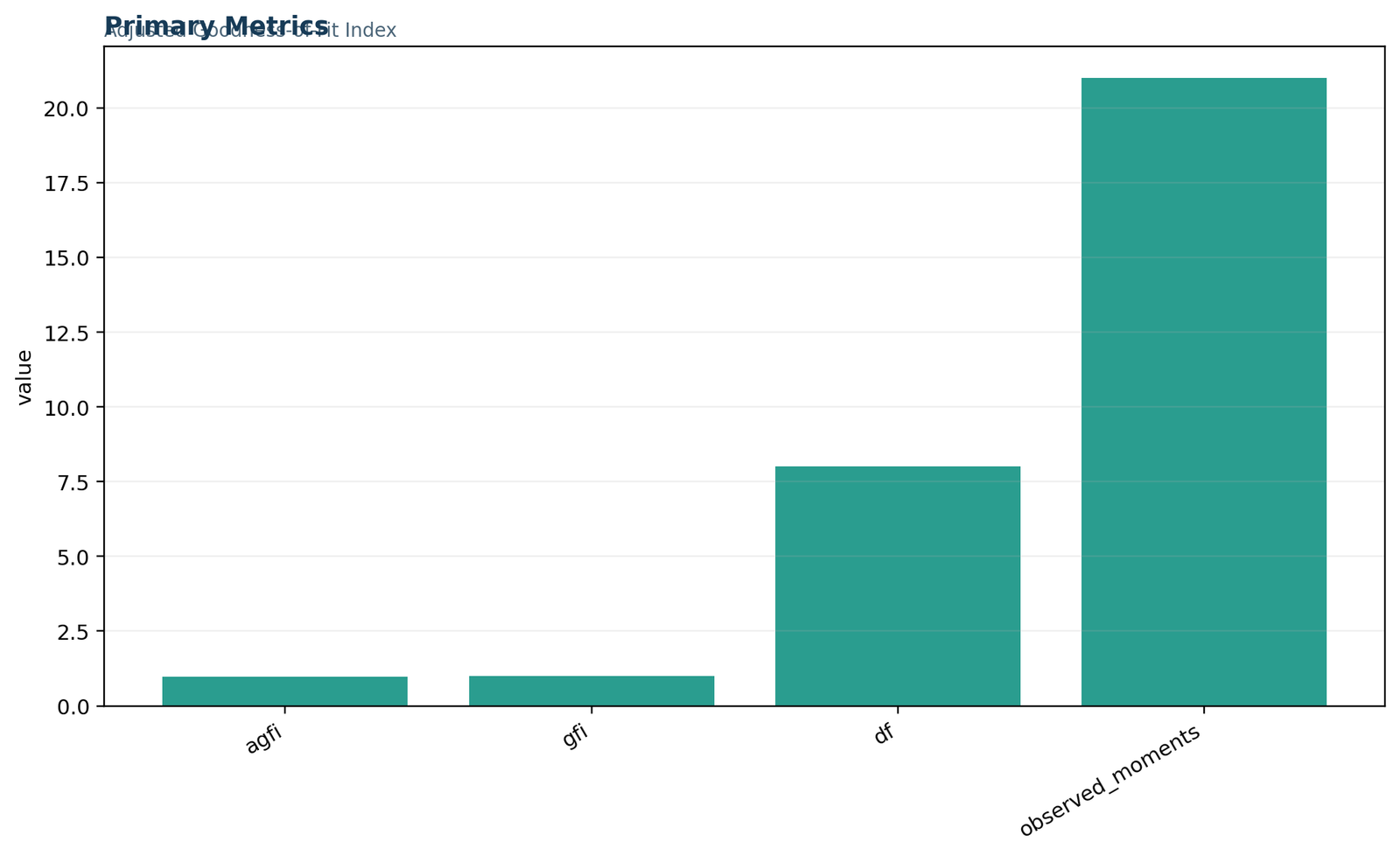
Python AGFI primary metrics
The first Python chart puts AGFI, GFI, model degrees of freedom and the number of observed covariance moments in one audit panel. Because the four quantities have very different scales, the chart should be read as a reporting inventory rather than as a magnitude comparison. The values to preserve are AGFI = 0.980667, GFI = 0.992635, df = 8 and 21 observed moments.
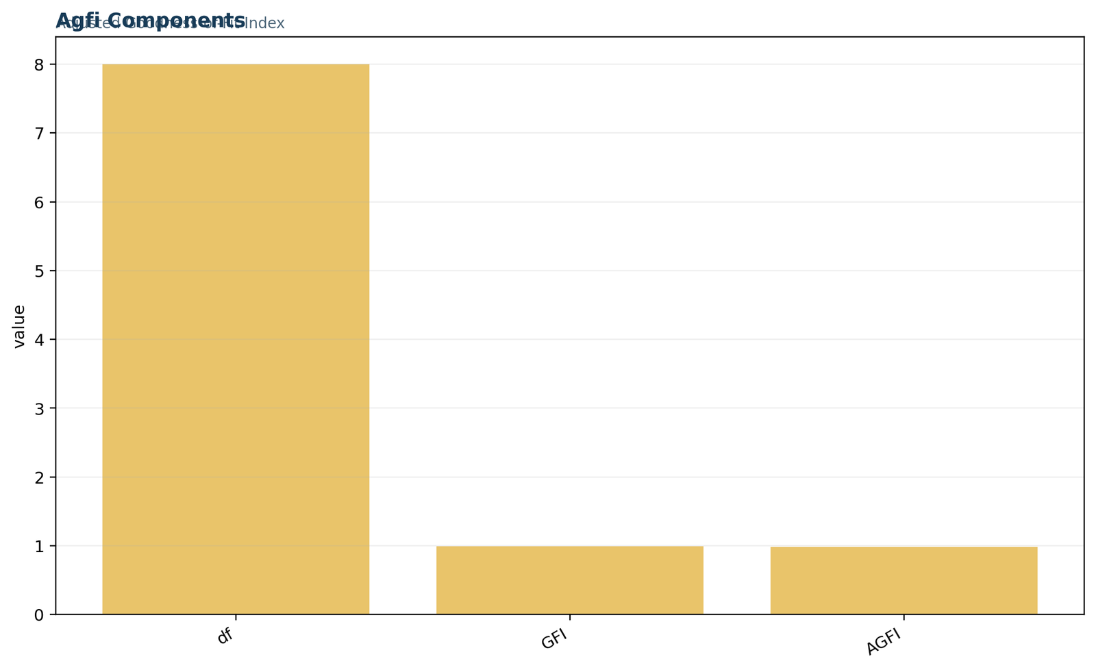
Python components of the AGFI adjustment
This component chart isolates the three quantities used in the adjusted goodness-of-fit calculation. The difference between GFI and AGFI is not an arbitrary software reduction: the GFI shortfall from one is multiplied by the complexity factor . That turns a raw lack-of-fit amount of 0.007365 into an adjusted amount of 0.019333.
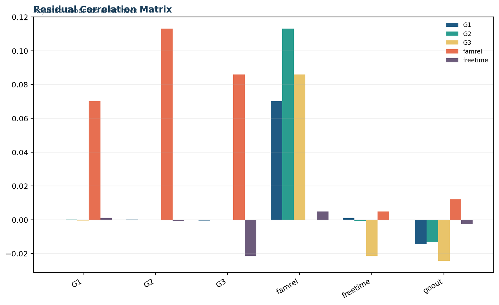
Python residual correlation matrix
The residual-correlation display is the most diagnostic chart in the Python report. The largest absolute residual is approximately 0.113 for G2 with famrel, followed by about 0.086 for G3 with famrel and 0.070 for G1 with famrel. These values show where the two-factor model leaves local association unexplained even though the global AGFI is high.
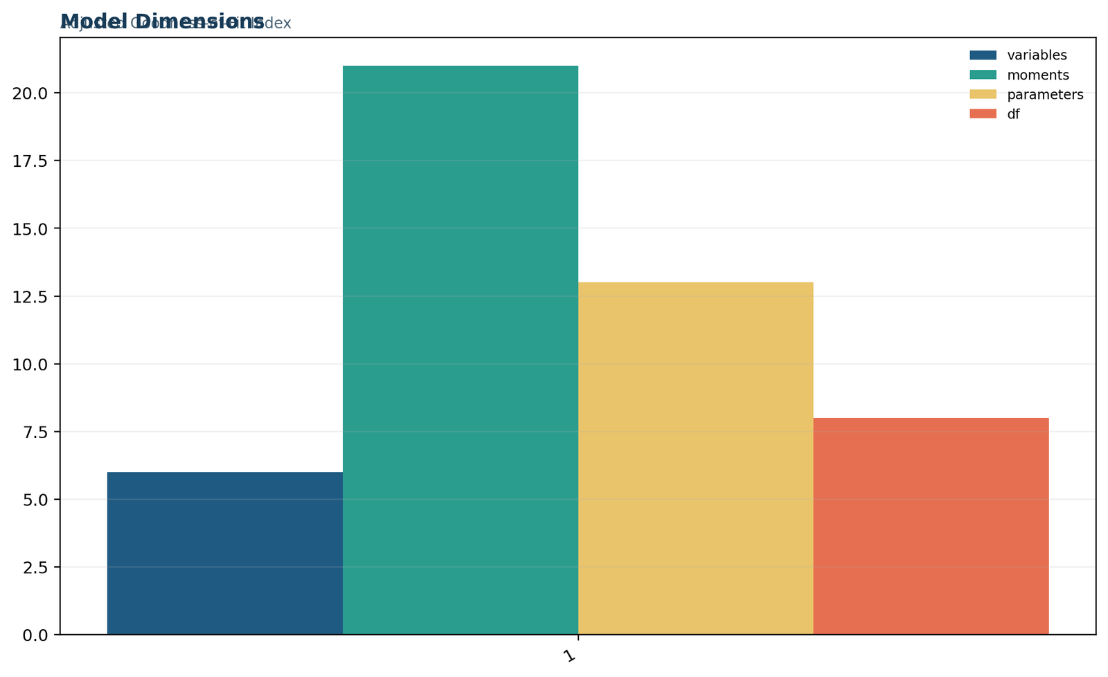
Python model dimensions
The model-dimension chart verifies identification arithmetic: six observed variables create 21 unique variances and covariances; 13 parameters are estimated; the difference is eight degrees of freedom. A reader can therefore reproduce the denominator used by the AGFI penalty instead of accepting df as an unexplained output number.
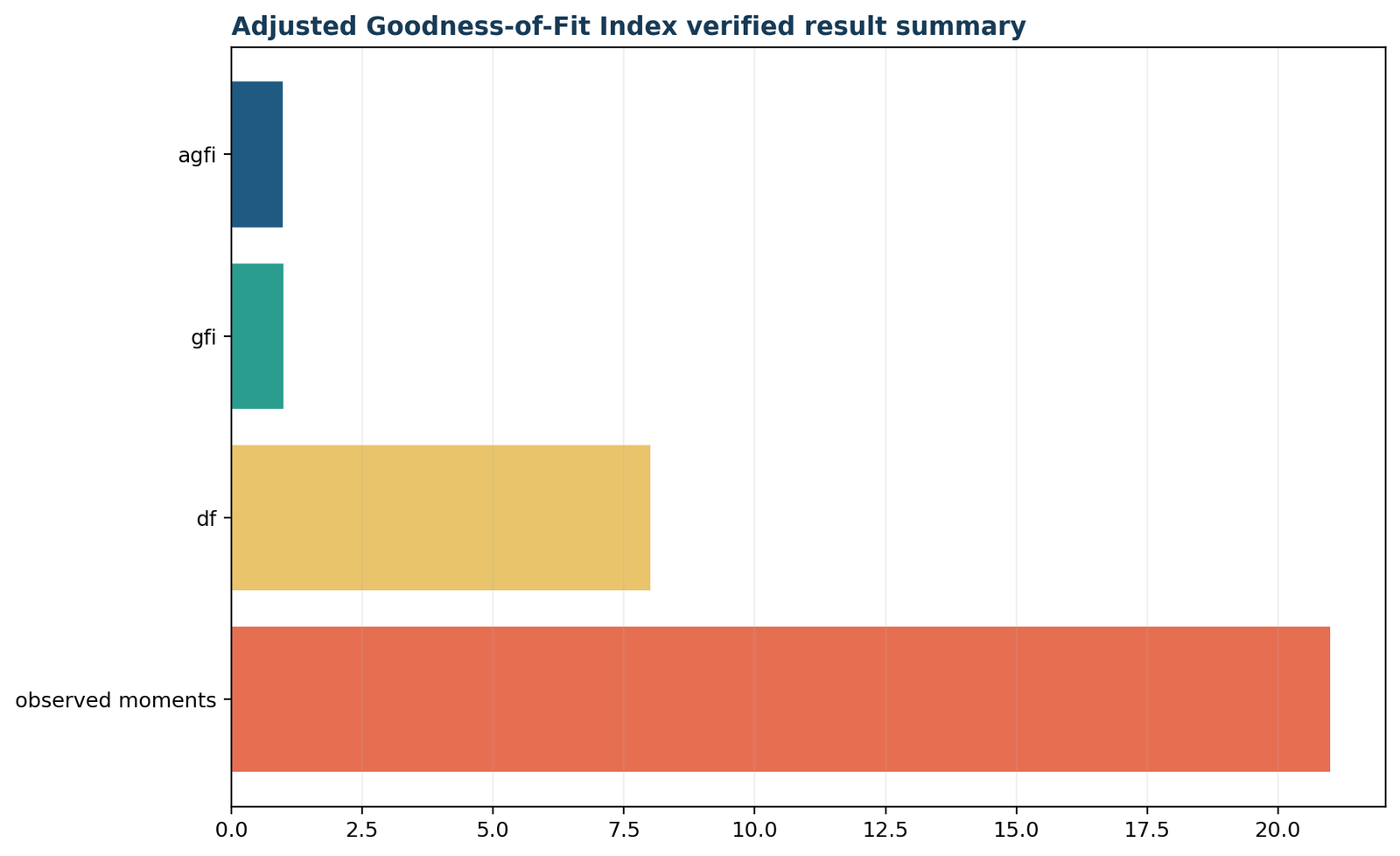
Python verified result summary
The final Python chart repeats the complete verification set and is designed for cross-software reconciliation. Agreement among the report, manual formula, PDF table and software output is more important than displaying many decimal places. Use 0.981 for prose, while keeping the full value in downloadable results.
AGFI versus GFI, CFI, TLI, RMSEA and SRMR
A high AGFI should be read as part of a complementary model-fit profile.
| Index | Fit family | Direction of better fit | What it adds beyond AGFI | Reporting caution |
|---|---|---|---|---|
| GFI | Absolute fit | Closer to 1 | Unadjusted covariance-reproduction summary | Can favor more complex models |
| AGFI | Adjusted absolute fit | Generally closer to 1 | Penalizes GFI shortfall using df | Historical cutoffs are not universal |
| CFI | Incremental fit | Closer to 1 | Compares target model with baseline model | Depends on baseline-model misfit |
| TLI | Incremental/parsimony | Closer to 1 | Stronger complexity sensitivity than CFI | Can exceed conventional bounds |
| RMSEA | Approximate fit | Closer to 0 | Includes df and supports interval estimates | Unstable in very low-df models |
| SRMR | Standardized residual fit | Closer to 0 | Directly summarizes standardized residual size | Averages can hide particular large residuals |
AGFI and GFI should not be confused with the categorical Chi square goodness of fit test despite the shared phrase “goodness of fit.” The chi-square goodness-of-fit test compares observed frequencies with expected frequencies, whereas AGFI evaluates a fitted covariance model.
APA-style reporting for Adjusted Goodness of Fit Index in Python
A complete sentence identifies the model, sample, software and limits of the conclusion.
Recommended reporting sentence
“A two-factor confirmatory factor analysis was estimated in Python for 649 observations. The Academic factor was measured by G1, G2 and G3, and the Social factor by famrel, freetime and goout. The model showed strong adjusted global fit, GFI = .993 and AGFI = .981, with 8 degrees of freedom. Residual-correlation inspection identified the largest local discrepancy between G2 and famrel (residual = .113), so global fit was interpreted alongside local diagnostics.”
Minimum technical details
Claims to avoid
Python AGFI troubleshooting
Common software-specific problems and the diagnostic action for each one.
| Problem | Likely cause or meaning | Recommended action |
|---|---|---|
| AGFI is missing from the output | Confirm that calc_stats(model) was called after a successful fit and that the returned table is indexed by Value. | Recheck the model specification, df, estimator, full-precision inputs and documented software behavior before reporting. |
| AGFI differs from the manual worksheet | Check whether the Python package uses baseline-model df rather than , whether means are estimated, and whether the same GFI is being adjusted. | Recheck the model specification, df, estimator, full-precision inputs and documented software behavior before reporting. |
| The model has zero or negative df | Reduce free parameters or revise the model. AGFI is not meaningful for a saturated or underidentified specification. | Recheck the model specification, df, estimator, full-precision inputs and documented software behavior before reporting. |
| Results change after dropna() | Document the complete-case variables. Dropping rows on additional columns silently changes N and the covariance matrix. | Recheck the model specification, df, estimator, full-precision inputs and documented software behavior before reporting. |
| Residuals look large despite AGFI above .95 | Treat this as local misfit. Inspect the particular indicator pairs, modification evidence and theory rather than relying on the global index. | Recheck the model specification, df, estimator, full-precision inputs and documented software behavior before reporting. |
Advanced Python implementation notes
Freeze the environment before comparing numbers. Save the Python version, semopy version, pandas version, NumPy version and optimizer information with the result. Fit indices depend on the fitted solution, and tiny optimizer or dependency changes can alter the last decimals of GFI and AGFI. A requirements file or locked environment makes a cross-software discrepancy easier to diagnose. The objective is not to force every package to print identical digits; it is to ensure that the same model and data produce the same substantive conclusion and a traceable numerical path.
Control covariance conventions. Python functions may use maximum-likelihood covariance normalization or the sample covariance with an N − 1 divisor. A custom manual GFI calculation can therefore diverge from semopy even when the model parameters appear similar. Record how the observed covariance matrix was created, and avoid mixing DataFrame.cov() output with a package objective that uses a different normalization. When the manual check begins from the package-reported GFI, the AGFI arithmetic is stable; when GFI itself is reconstructed, covariance and discrepancy conventions become part of the specification.
Inspect baseline-model degrees of freedom. semopy’s documented AGFI calculation uses the baseline model’s df divided by the target model’s df. For this conventional six-variable covariance model, that route corresponds to the 21/8 multiplier used in the verification report. More complex models can break the apparent equivalence with a simple expression. Print DoF Baseline, DoF, GFI and AGFI together. If another library uses a different adjustment, label the implementation rather than silently replacing one result with the other.
Build a residual-pair audit table. Convert the symmetric residual correlation matrix into unique off-diagonal pairs, calculate absolute residuals, sort descending and attach interpretation flags. The first three pairs in the supplied model all involve famrel with an academic grade. This structured table is more useful than a heatmap alone because it can be filtered, exported and tested. A code assertion can verify that the matrix is symmetric, diagonal residuals are near zero and variable labels match the fitted covariance order.
Handle missing data deliberately. The worked code uses complete cases on exactly six columns. FIML or imputation would retain a different analysis sample and may change the fitted covariance structure. Never call dropna() on the full source table when unrelated variables contain missing values, because that discards cases that are complete for the CFA. Save the retained row identifiers and a missingness summary. When alternative models are compared, fit all of them to the same row set unless the analysis plan explicitly allows sample changes.
Separate model discovery from confirmation. Python makes it easy to loop over candidate cross-loadings and residual covariances, but selecting the model with the largest AGFI on the same sample inflates optimism. Use theory to define a small candidate set, reserve validation data when feasible, and report the original specification even if a revised model is explored. Automated search can be useful for diagnostics, but it should not convert a confirmatory factor analysis into an undocumented specification-mining exercise.
Check admissibility before chart generation. A pipeline should not create polished figures when the solution contains negative residual variances, nonfinite standard errors, an impossible latent correlation or failed convergence. Validate the fitted object first, then calculate statistics and visuals. Include the optimizer status in the PDF. This prevents a high AGFI from being visually promoted when the parameter solution is statistically unacceptable.
Use unit tests for the published result. Store expected quantities—N = 649, p = 6, moments = 21, parameters = 13, df = 8, GFI near 0.992635 and AGFI near 0.980667—in a small test module. Tests should allow a defensible numerical tolerance while rejecting large changes caused by wrong columns, row filtering or model edits. Reproducible analytical content benefits from the same regression-testing logic used in software engineering: when code changes, the result should either remain within tolerance or trigger a documented review.
Python validation checklist and interpretation scenarios
Scenario 1: semopy reports a high AGFI and the optimizer succeeded. Continue to inspect parameter admissibility. Successful numerical convergence means the optimizer found a solution, not that every variance, covariance and loading is scientifically acceptable. Build checks for negative residual variances, nonfinite estimates and factor correlations beyond plausible bounds before exporting charts or an APA sentence.
Scenario 2: AGFI is high but the residual matrix has a visible cluster. The current famrel–grade residuals illustrate this case. Use a long-form residual table and group pairs by measurement block. A cluster across factors can indicate an omitted cross-loading, a direct relationship, a weak factor definition or a sample-specific pattern. The software identifies the location; theory determines the response.
Scenario 3: Python and R differ in the seventh decimal. Compare full-precision GFI, target df and baseline df before investigating deeper causes. The supplied results differ by roughly two ten-millionths and round identically. Such a difference is not a substantive conflict. A discrepancy in the third decimal, however, would justify checking data rows, covariance normalization, model constraints and package definitions.
Scenario 4: adding a residual covariance improves GFI. Recalculate q and df automatically. The revised model’s AGFI should be computed from its own fit and complexity, not by reusing the original df. Store both models in a comparison DataFrame and include the theoretical reason for the added covariance. A loop that frees paths solely by largest modification evidence is exploratory model search.
Scenario 5: columns are read as strings. pandas can import numeric-looking fields as object type when files contain stray characters. Coerce the six analysis variables explicitly, count conversion failures and stop if unexpected missing values are created. A covariance model built from silently altered columns can still run and produce persuasive output, making type validation an essential pre-fit step.
Scenario 6: feature scaling is changed. Covariance-based fit can respond to scale conventions, while standardized residual interpretation depends on correct standardization. Do not standardize some indicators and leave others raw unless that is the planned model. If all indicators are standardized for a correlation-model analysis, label the method and do not compare its GFI directly with a raw-covariance result.
Scenario 7: FIML or imputation is introduced. Save an analysis flag describing the missing-data path and ensure the PDF states it. Imputed datasets may require pooled parameter and fit treatment rather than one completed file treated as observed truth. The complete-case result in this post is simple to reproduce because exactly six columns define row inclusion.
Scenario 8: a dashboard displays AGFI as 98.1%. Correct the label. Multiplying by 100 can be visually convenient, but it encourages the false claim that the model explains 98.1% of variance. Keep the axis and card labeled “AGFI” and display .981. Explain that it is an adjusted covariance-reproduction index, not a percentage of outcome variance.
Scenario 9: the result is deployed in a web calculator. Require users to provide either p and df with a validated GFI or p and q with GFI. Validate df > 0, retain full precision, show all intermediate steps and warn that the calculator does not estimate a CFA. The calculation engine should be separate from the explanatory content and should reproduce the worked result exactly.
Scenario 10: the pipeline is rerun after code changes. Unit tests should confirm row count, variable order, moment count, df, GFI, AGFI and the identity of the largest residual pair. Snapshot tests can verify that tables contain the expected labels. This converts the statistical report into a maintainable analytical product rather than a one-time notebook.
Limitations of Adjusted Goodness of Fit Index in Python
What this index, software route and worked model cannot establish.
For numerical reproducibility, store the raw covariance matrix and model-implied covariance matrix as labeled pandas DataFrames. Variable order must remain identical. A residual matrix calculated after columns are reordered can look plausible while pairing the wrong indicators. Exporting both matrices to CSV creates an audit trail that is easier to compare with R or Amos than screenshots alone.
Optimizer success is necessary but not sufficient. Review parameter estimates for negative residual variances, factor correlations outside the admissible range, extremely large standard errors and boundary estimates. A high AGFI from an inadmissible solution is not evidence of acceptable fit. Programmatic assertions can halt the reporting pipeline when df is nonpositive, convergence fails or the covariance matrix is not positive definite.
When comparing alternative Python models, keep the analysis rows fixed. If each candidate model drops missing values only from its own variables, the covariance matrices and sample sizes differ; a change in AGFI then reflects both model specification and sample composition. Construct one comparison frame containing every variable used by any candidate model before fitting the set.
Do not infer that semopy and lavaan must match at every decimal. Packages can differ in objective scaling, covariance normalization, baseline-model construction and optimization tolerances. Reconciliation should begin with p, q, df, GFI definition and estimator. A two-millionth AGFI difference is negligible when both results round to .981 and the local residual pattern agrees.
Python libraries do not all define GFI and AGFI in exactly the same computational family. semopy uses its documented baseline-model degrees-of-freedom adjustment. A custom covariance-discrepancy implementation can reproduce the supplied value only when it uses the same GFI definition, estimator, model specification, variable order and treatment of means. Name the package and version in a reproducible report rather than writing only “Python was used.”
Global averaging
AGFI compresses many covariance discrepancies into one number. Local residuals and weak indicators can remain hidden.
Model equivalence
Different factor structures can sometimes reproduce the same or nearly the same covariance matrix.
Cutoff dependence
The .90 rule is a convention, not a theorem. Model size, df, estimator and sample conditions matter.
Sample dependence
The index describes fit in the analyzed sample. Replication or cross-validation is needed for generalization.
Reliability separation
Good covariance fit does not guarantee reliable scales. The weak social alpha in this example illustrates the distinction.
Causal limits
A CFA fit index does not prove causal relations among factors or indicators.
Adjusted Goodness of Fit Index in Python downloads and reproducibility files
Use the method-specific file first; supporting files are included for cross-checking.
Adjusted Goodness of Fit Index in Python frequently asked questions
Direct answers to software, formula, interpretation and reporting questions.
What is the Adjusted Goodness of Fit Index?
AGFI is a model-fit index derived from GFI with an adjustment for the degrees of freedom available to test a covariance-structure model. It summarizes global covariance reproduction with a complexity penalty.
Is AGFI a statistical test?
No. AGFI is a descriptive fit index. It does not have the same interpretation as a p-value and should not be reported as if a null hypothesis were directly accepted or rejected by the index.
What is a good AGFI value?
Larger values generally indicate better global fit, and .90 is often used as a historical rule of thumb. A fixed cutoff is not a universal law. Estimator, model size, indicator quality, residuals and the complete fit profile must be considered.
Can AGFI be higher than GFI?
Under the conventional positive-df adjustment, AGFI is usually less than or equal to GFI because the GFI shortfall is multiplied by a factor related to complexity. Unusual implementations or pathological models require formula verification.
Why does AGFI decrease when paths are added?
Adding free parameters reduces degrees of freedom. Even if raw fit improves, the parsimony adjustment can offset part of that improvement.
Can AGFI be negative?
Yes, some formulations can produce negative values for very poor-fitting or low-df models. Do not truncate the value silently; investigate model specification and the software definition.
Should AGFI be reported alone?
No. Report it with the model chi-square and df plus complementary indices such as CFI, TLI, RMSEA and SRMR, and include local residual or parameter diagnostics.
Does a high AGFI prove the model is correct?
No. Many different models can reproduce a covariance matrix well. Fit is necessary evidence for a proposed model, not proof of causal truth, construct validity or unique specification.
What does df = 8 mean here?
Six observed variables provide 21 unique covariance moments. The model estimates 13 free parameters, leaving 21 − 13 = 8 degrees of freedom for evaluating global fit.
Why are G1, G2 and G3 grouped together?
They are repeated academic performance measures with strong correlations in the supplied data. The model treats them as indicators of an Academic latent factor.
Why inspect the residual correlation matrix?
A global index can look excellent while specific indicator pairs remain under- or over-reproduced. Residuals locate those local discrepancies.
How should AGFI be rounded?
Use three decimals in ordinary prose, for example AGFI = .981, while retaining more precision in tables, code output and downloadable verification files.
Which Python package calculates AGFI?
semopy provides GFI and AGFI through calc_stats(). Always cite the package and preserve the model specification because formulas can differ among libraries.
How do I print only AGFI in Python?
After calc_stats(model), select the Value row and AGFI column. Also print DoF and GFI so the number remains auditable.
Can statsmodels calculate this AGFI directly?
statsmodels is not a general latent-variable SEM package with the same GFI/AGFI output. Use a dedicated SEM implementation or a validated custom calculation.