
Categorical Association, Chi-Square, Crosstabs, Residuals and Effect Size
Contingency Coefficient: Formula, Interpretation, SPSS, Python, R and Excel Guide
Contingency Coefficient is an effect-size measure for the association between two categorical variables. It is calculated from the Pearson chi-square statistic and is often reported with a contingency table, observed counts, expected counts, row percentages, standardized residuals and cell contributions. This guide explains the contingency coefficient formula, interpretation rules, SPSS output, Python charts, R validation charts, Excel worked results, APA wording, common mistakes and downloadable resources.
Quick Answer: Contingency Coefficient Result
The worked example tested whether school and sex were associated in the student performance dataset. The crosstab contained N = 649 valid students. The observed table showed GP school: 237 F and 186 M, and MS school: 146 F and 80 M. The Pearson chi-square result was χ²(1) = 4.4763, with p = .0344.
The Contingency Coefficient was C = 0.0828. Because C has a maximum below 1 for finite tables, the Excel workbook also calculated the maximum possible value for this 2 × 2 table as Cmax = 0.7071 and the adjusted coefficient as adjusted C = 0.1170. Cramer’s V and Phi were both approximately 0.0830. The result is statistically significant at the .05 level, but the association is weak in practical strength.
Final interpretation: The school and sex variables are not perfectly independent in this sample. However, the strength is weak. GP has a larger male share than MS, while MS has a larger female share than expected under independence. The statistical decision is significant, but the effect-size decision is weak.
Important reporting point: A significant chi-square test does not automatically mean a strong association. With large samples, small differences in a crosstab can become statistically significant. Always report the Contingency Coefficient, adjusted C, Cramer’s V or Phi with the p-value.
Table of Contents
- What Is a Contingency Coefficient?
- Contingency Coefficient Formula
- Null and Alternative Hypotheses
- Dataset and Variables Used
- SPSS Output Interpretation
- Python Chart-by-Chart Interpretation
- R Chart-by-Chart Validation
- Excel Results Explained
- SPSS, R, Python and Excel Workflows
- Code Blocks for Contingency Coefficient
- APA Reporting Wording
- Common Mistakes
- When to Use Contingency Coefficient
- Downloads and Resources
- Related Guides
- FAQs
What Is a Contingency Coefficient?
The Contingency Coefficient, often written as C, measures the strength of association between two categorical variables. It is based on the Pearson chi-square statistic from a contingency table. If the observed counts are very close to the expected counts under independence, C is close to 0. If the observed counts depart more strongly from expected counts, C becomes larger.
A contingency table is a cross-classification of two categorical variables. In this example, the row variable is school with two categories, GP and MS. The column variable is sex with two categories, F and M. The test asks whether the distribution of sex is the same inside both school categories.
The Contingency Coefficient belongs to the same family of categorical association measures as Phi and Cramer’s V. For a 2 × 2 table, Phi and Cramer’s V are often easier to compare because they use a 0 to 1 scale. The unadjusted Contingency Coefficient has a maximum below 1, so the adjusted C is useful when comparing results across tables of different sizes.
Simple definition: Contingency Coefficient tells how strongly two categorical variables are associated after a chi-square test. In this post, school and sex are significantly associated, but the effect size is weak.
Before interpreting C, it helps to understand cross tabulation, frequency distribution, p-value, effect size and null and alternative hypothesis reporting.
Contingency Coefficient Formula
The Contingency Coefficient is calculated from Pearson’s chi-square statistic and the total sample size:
For the worked example, χ² = 4.4763 and N = 649. Substituting those values gives C = √[4.4763 / (4.4763 + 649)] = 0.0828. This is a weak association.
Because the maximum value of C depends on the number of categories in the smaller dimension of the table, an adjusted value can also be calculated:
In a 2 × 2 table, k = 2, so Cmax = √(1/2) = 0.7071. The adjusted value is 0.0828 / 0.7071 = 0.1170. The adjusted value is still weak.
| Symbol | Meaning | Value in This Example |
|---|---|---|
| χ² | Pearson chi-square statistic | 4.4763 |
| N | Total valid sample size | 649 |
| C | Contingency Coefficient | 0.0828 |
| k | Smaller number of row or column categories | 2 |
| Cmax | Maximum possible C for the table size | 0.7071 |
| Adjusted C | C divided by Cmax | 0.1170 |
The chi-square statistic itself comes from observed and expected counts:
Expected counts are calculated as row total multiplied by column total divided by the grand total. The same logic is used in SPSS, Python, R and Excel.
Null and Alternative Hypotheses for Contingency Coefficient
The Contingency Coefficient itself is an effect-size statistic. The significance decision comes from the chi-square test of independence that produces the chi-square statistic used in the formula.
| Statement | Hypothesis | Meaning |
|---|---|---|
| Null hypothesis | H0: school and sex are independent | The distribution of F and M is the same across GP and MS. |
| Alternative hypothesis | H1: school and sex are associated | The distribution of F and M differs by school category. |
| Effect-size interpretation | C > 0 | The variables show some level of categorical association. |
Decision for this example: Because p = .0344 is below .05, the independence null hypothesis is rejected. However, C = .0828 and adjusted C = .1170 show that the association is weak.
Dataset and Variables Used
The worked example uses the student performance dataset. The main contingency table compares school and sex. The row variable is school, with categories GP and MS. The column variable is sex, with categories F and M. The analysis uses 649 valid cases.
| Variable | Role | Categories | Why It Matters |
|---|---|---|---|
| school | Row categorical variable | GP, MS | Defines the school groups being compared. |
| sex | Column categorical variable | F, M | Defines the distribution being compared inside each school. |
| Observed counts | Crosstab frequencies | 237, 186, 146, 80 | Actual number of students in each school-by-sex cell. |
| Expected counts | Independence model counts | 249.63, 173.37, 133.37, 92.63 | Counts expected if school and sex were independent. |
| Cell residuals | Observed minus expected pattern | Positive and negative departures | Shows which cells explain the chi-square result. |
For categorical data, it is useful to report both the raw counts and row percentages. Raw counts show sample size. Row percentages show how the column distribution changes across row categories. This is why a complete report should include a descriptive statistics section, a crosstab section and an effect size section.
SPSS Output Interpretation for Contingency Coefficient
The SPSS output verifies the same crosstab result using CROSSTABS. SPSS reports the observed counts, expected counts, row percentages, Pearson chi-square test and symmetric measures such as Phi, Cramer’s V and the Contingency Coefficient.
| SPSS Output Item | Value | Interpretation |
|---|---|---|
| Valid N | 649 | All valid school-by-sex cases were included. |
| Observed GP-F | 237 | F students in GP school. |
| Observed GP-M | 186 | M students in GP school. |
| Observed MS-F | 146 | F students in MS school. |
| Observed MS-M | 80 | M students in MS school. |
| Pearson chi-square | χ²(1) = 4.4763 | The crosstab departs from perfect independence. |
| p-value | .0344 | The association is statistically significant at α = .05. |
| Contingency Coefficient | .0828 | The association strength is weak. |
| Adjusted C | .1170 | Still weak after correcting for the maximum possible C. |
| Cramer’s V / Phi | .0830 | Confirms a weak 2 × 2 categorical association. |
SPSS Observed and Expected Counts
| Cell | Observed Count | Expected Count | Observed – Expected | Interpretation |
|---|---|---|---|---|
| GP × F | 237 | 249.63 | -12.63 | F students are lower than expected in GP. |
| GP × M | 186 | 173.37 | +12.63 | M students are higher than expected in GP. |
| MS × F | 146 | 133.37 | +12.63 | F students are higher than expected in MS. |
| MS × M | 80 | 92.63 | -12.63 | M students are lower than expected in MS. |
SPSS interpretation summary: SPSS supports the same conclusion as Excel, Python and R. There is a statistically significant association between school and sex, but the effect size is weak. The pattern is mainly that GP has more M students than expected and MS has fewer M students than expected under independence.
Python Chart-by-Chart Interpretation
The Python charts explain the contingency coefficient from several angles: row percentages, observed counts, standardized residuals, chi-square cell contributions, effect-size summary and observed-versus-expected counts. Together, these charts show not only whether the association is significant, but where it comes from and how strong it is.
Python Chart 1: Row Percentage Profile

This chart converts the school-by-sex table into row percentages. GP is about 56.0% F and 44.0% M, while MS is about 64.6% F and 35.4% M. The blue F section is taller in MS, and the orange M section is taller in GP. That visible shift is the practical pattern behind the significant chi-square result.
The chart also shows why the effect is weak. Both schools still contain large numbers of F and M students; the categories do not separate sharply. The difference is an 8 to 9 percentage-point shift in group composition, not a dramatic change. This supports the conclusion that the association is statistically significant but weak in strength.
Python Chart 2: Observed Count Heatmap
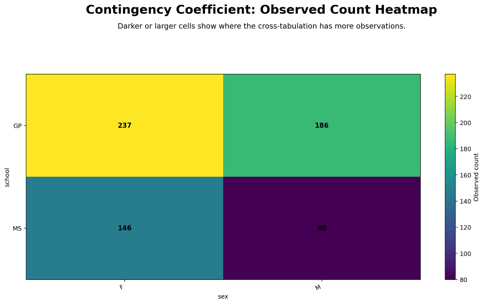
The heatmap displays the four observed cell counts: GP-F = 237, GP-M = 186, MS-F = 146 and MS-M = 80. The largest cell is GP-F, and the smallest cell is MS-M. This is expected partly because GP has more students overall than MS and because F students are more common than M students in the full dataset.
Raw counts alone do not prove association because larger row totals naturally create larger counts. That is why the next charts compare observed counts with expected counts. The heatmap is still important because it gives the reader the actual data structure before the chi-square and contingency coefficient are interpreted.
Python Chart 3: Standardized Residual Map
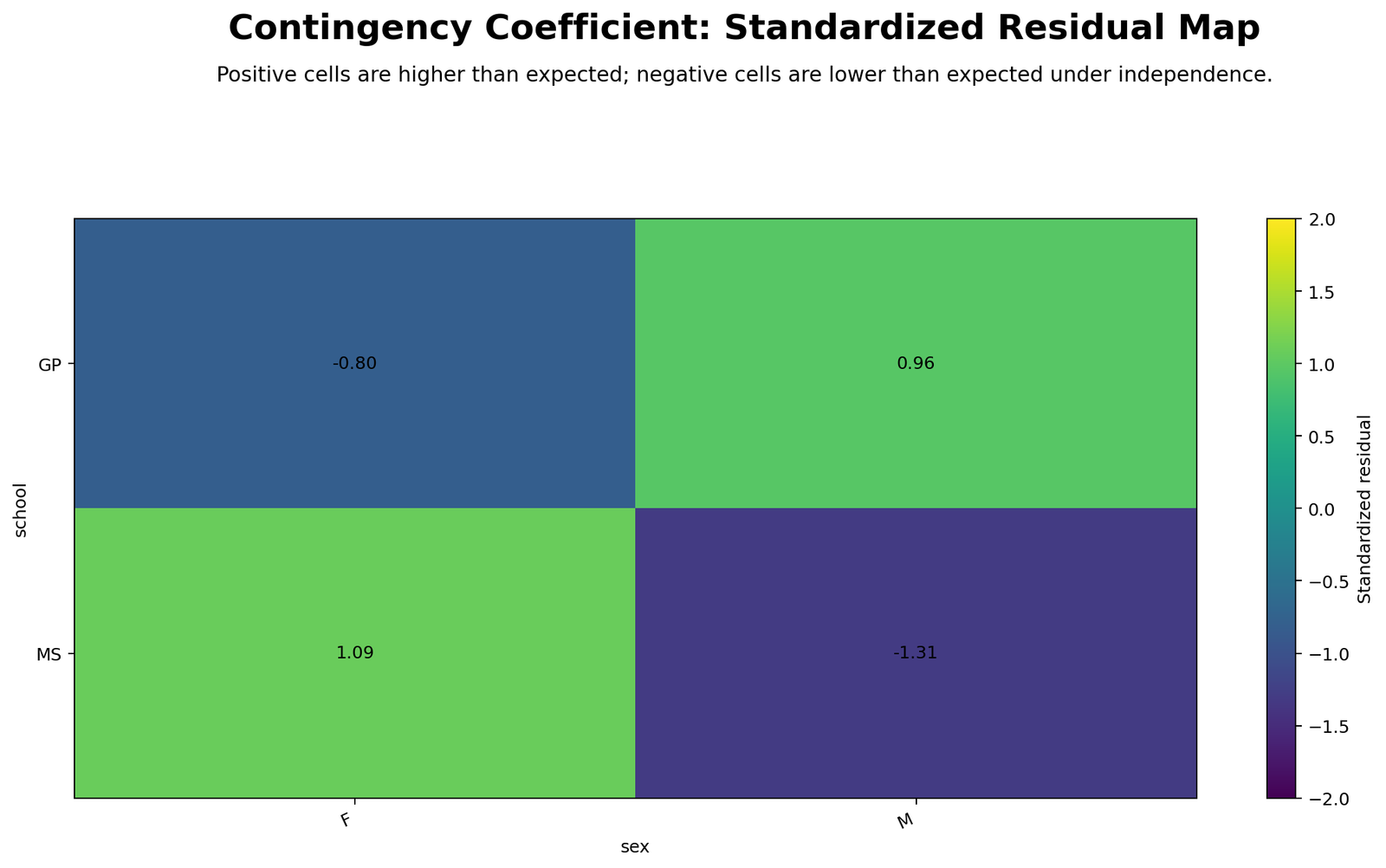
The residual map explains direction. The GP-F cell is negative (-0.80), meaning fewer F students were observed in GP than expected. The GP-M cell is positive (0.96), meaning more M students were observed in GP than expected. The MS-F cell is positive (1.09), and the MS-M cell is negative (-1.31).
No residual reaches the common ±2 review threshold. This is a key result. The table is significant overall, but no single cell is an extreme departure from independence. The largest standardized residual in absolute value is MS-M at about -1.31, so the evidence is distributed across the 2 × 2 pattern rather than dominated by one extreme cell.
Python Chart 4: Chi-Square Cell Contributions
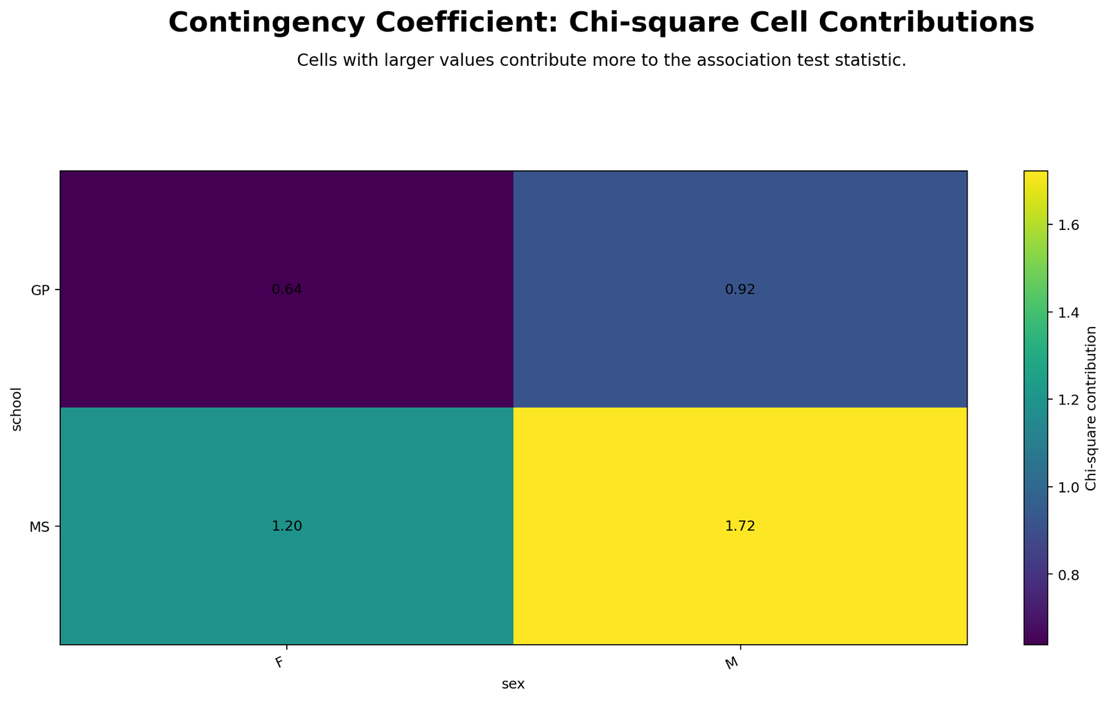
This chart shows how much each cell contributes to the total chi-square value. The cell contributions are approximately 0.64 for GP-F, 0.92 for GP-M, 1.20 for MS-F and 1.72 for MS-M. The MS-M cell is the largest contributor because the observed count of 80 is meaningfully below its expected count of about 92.63.
The contribution chart is more specific than the p-value. It tells the analyst where the association comes from. In this example, the pattern is mainly that MS has fewer M students and more F students than the independence model would expect, while GP shows the opposite direction.
Python Chart 5: Association Strength Summary
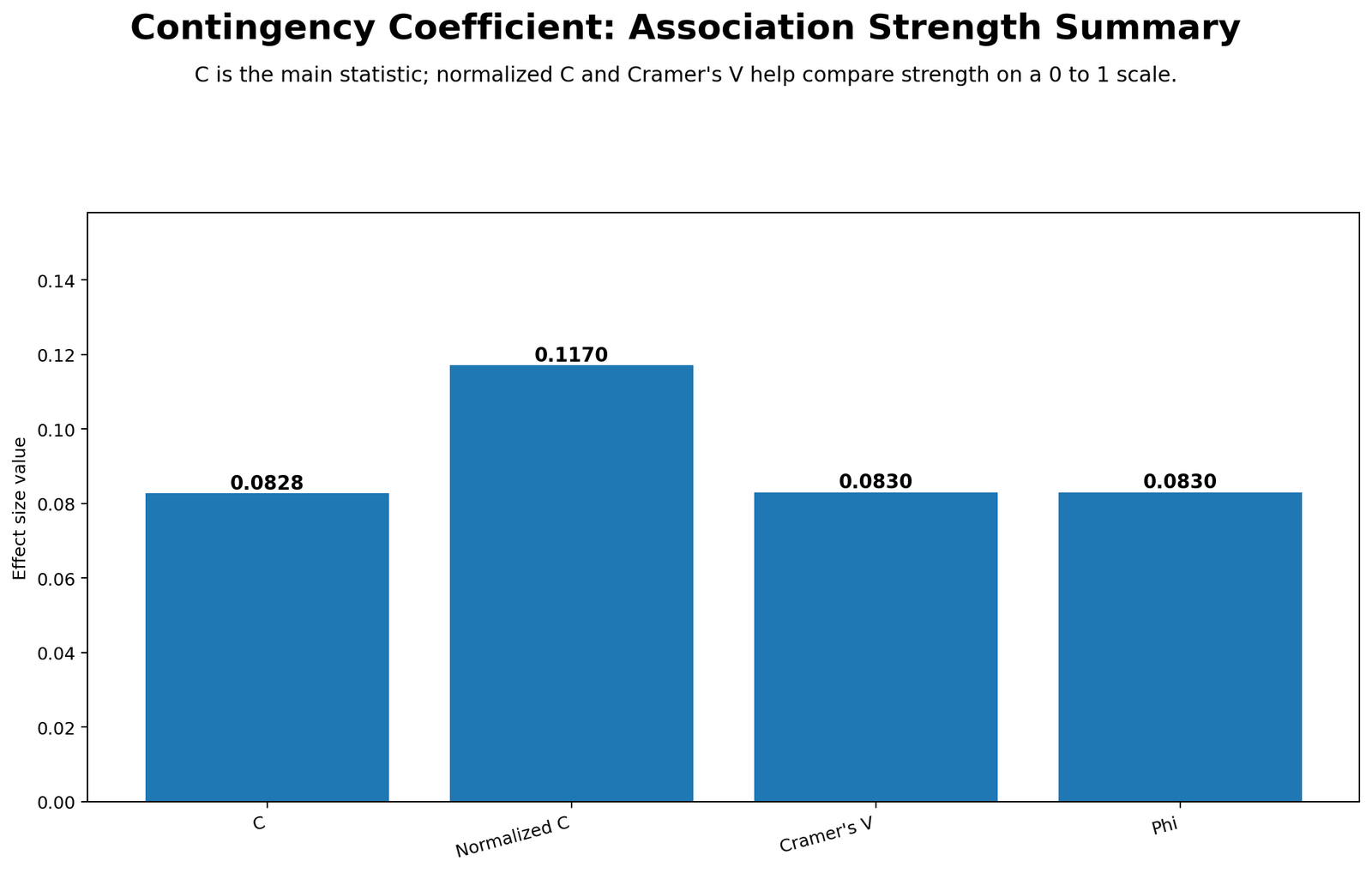
The effect-size chart puts the strength statistics side by side. The unadjusted Contingency Coefficient is 0.0828, normalized C is 0.1170, Cramer’s V is about 0.0830 and Phi is about 0.0830. All values are close to zero.
This chart prevents overclaiming. The p-value is below .05, but the effect size is clearly small. The correct report should say that the school-by-sex association is significant but weak, not that school strongly determines sex distribution.
Python Chart 6: Observed vs Expected Counts
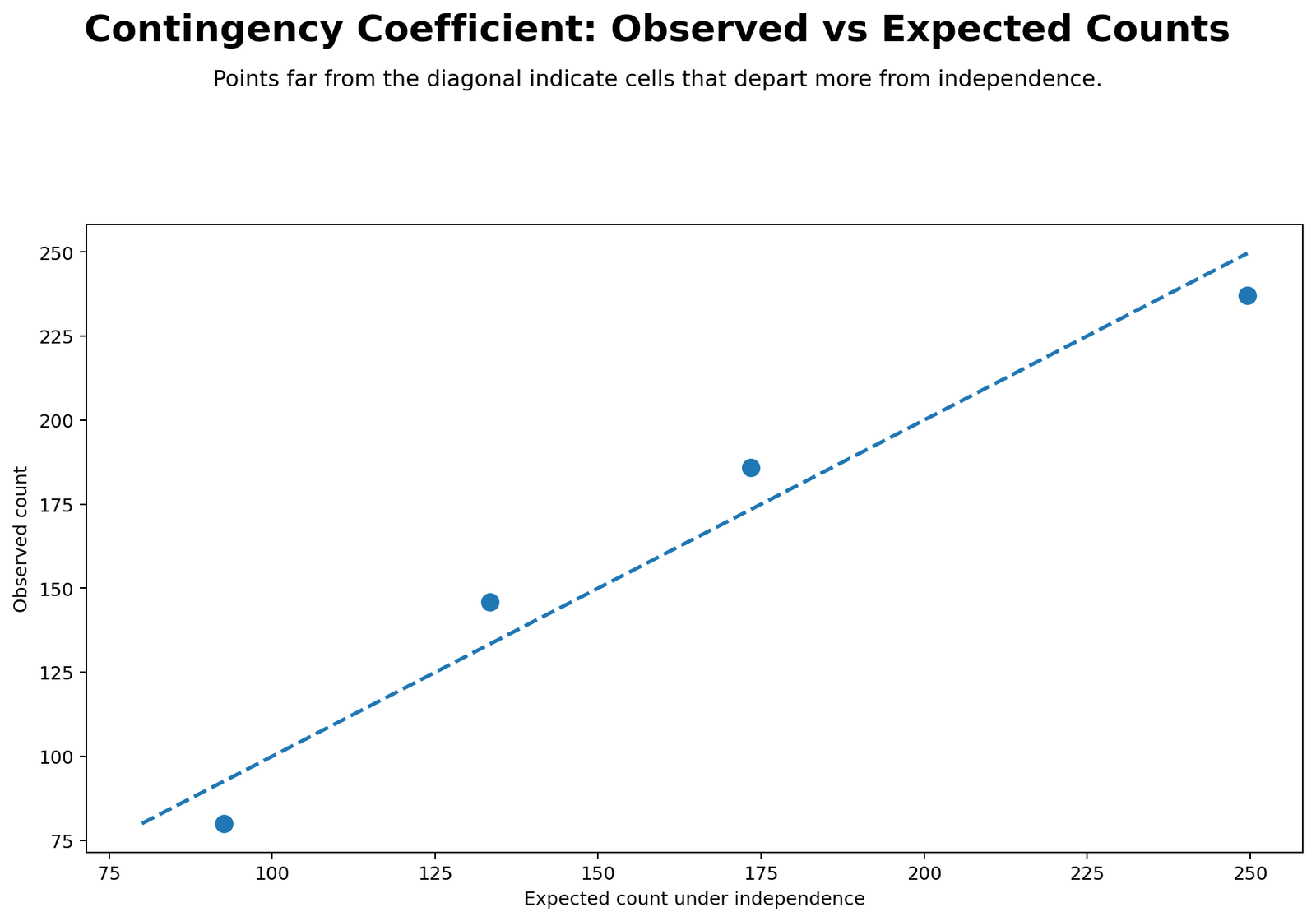
The dashed diagonal represents perfect agreement between observed and expected counts. The GP-F point is below the diagonal because 237 observed is lower than 249.63 expected. The GP-M point is above the diagonal because 186 observed is higher than 173.37 expected. The MS-F point is also above the diagonal, while the MS-M point is below it.
The points are not far away from the diagonal, which again supports a weak association. The plot is useful because it turns the expected-count logic into a simple visual: the closer the points are to the diagonal, the closer the table is to independence.
R Chart-by-Chart Validation
The R charts validate the same contingency coefficient result with a separate workflow. They repeat the row percentage profile, observed count heatmap, standardized residuals, chi-square contributions, effect-size summary and observed-versus-expected counts in a colorful report style. This agreement across Python, R, SPSS and Excel strengthens the interpretation.
R Chart 1: Row Percentage Profile

The R row-percentage chart confirms the Python pattern. MS has a higher F share and lower M share than GP. This is the visible association that the chi-square test detects. The difference is real but not large, which is why the adjusted C remains low.
This chart is the clearest chart for nontechnical readers because percentages are easier to compare than raw frequencies when row totals differ.
R Chart 2: Observed Count Heatmap

The R heatmap confirms the same observed counts. GP-F is the largest cell and MS-M is the smallest cell. This raw table structure matters because every later statistic is built from these counts.
Because row totals are unequal, the raw count chart should not be interpreted alone. It should be read with row percentages, expected counts and residuals.
R Chart 3: Standardized Residual Map

The R residual chart validates the same four-cell direction pattern: GP-F is below expected, GP-M is above expected, MS-F is above expected and MS-M is below expected. The largest absolute residual is still modest, so no cell should be described as extremely unusual.
This is the best chart for explaining the direction of association because positive and negative residuals show which cells drive the deviation from independence.
R Chart 4: Chi-Square Cell Contributions

The R contribution chart again shows that MS-M contributes the most to the chi-square statistic, followed by MS-F, GP-M and GP-F. This confirms the Python conclusion that the MS row contains the stronger departure from expected sex counts.
The chart also shows why the overall chi-square value is not large. The contributions add up to about 4.476, which is just enough to reach significance with one degree of freedom.
R Chart 5: Association Strength Summary

The R effect-size chart confirms the weak-strength conclusion. C, Cramer’s V and Phi are all close to .08, while adjusted C is about .117. These values are far closer to zero than to a moderate or strong association.
This is the chart that should guide the strength language in the final report. The p-value answers whether the variables are independent; this chart answers how strong the association is.
R Chart 6: Observed vs Expected Counts

The R observed-versus-expected plot confirms that all four cells are close to the independence line. Two cells are above expected and two cells are below expected. The departures are coordinated enough to produce a significant test, but not large enough to support a strong practical association.
This chart is helpful for final checking because it shows the complete expected-count logic in one figure.
Excel Results Explained
The uploaded Excel workbook gives a fully worked formula-based calculation for the same school × sex crosstab. It includes a dashboard, raw data, categorical data, observed table, expected counts, chi-square components, main worked calculation, pairwise categorical results and an Excel guide.
Excel Main Worked Result: school × sex
| Excel Item | Value | Interpretation |
|---|---|---|
| Row variable | school | The two school categories are GP and MS. |
| Column variable | sex | The two sex categories are F and M. |
| Valid N | 649 | All valid crosstab cases were included. |
| Observed table | GP-F 237, GP-M 186, MS-F 146, MS-M 80 | The actual frequency table used for the chi-square test. |
| Expected table | 249.63, 173.37, 133.37, 92.63 | The counts expected if school and sex were independent. |
| Chi-square | 4.4763 | Total of all chi-square cell components. |
| Degrees of freedom | 1 | (rows − 1) × (columns − 1). |
| p-value | 0.034368 | Significant association at α = .05. |
| Contingency C | 0.0828 | Weak categorical association. |
| Maximum possible C | 0.7071 | The largest possible C for a 2 × 2 table. |
| Adjusted C | 0.1170 | Weak after maximum-C adjustment. |
The Excel workbook shows exactly how the result is built. The largest chi-square component is the MS × M cell at approximately 1.72, followed by MS × F at 1.20, GP × M at 0.92 and GP × F at 0.64. This means the MS row contributes slightly more to the association pattern than the GP row.
The workbook’s dashboard interpretation is: Pearson chi-square = 4.4763, df = 1, p-value = 0.034368, C = 0.0828, adjusted C = 0.1170. The decision is significant at .05, but the strength is weak. This is the strongest way to report the result because it combines statistical significance with practical strength.
Excel Pairwise Results: Stronger Categorical Associations
The workbook also calculates many pairwise categorical associations. These are useful because they show how weak the main school-by-sex association is compared with stronger categorical relationships in the same dataset.
| Rank | Variable Pair | Chi-square | p-value | C | Adjusted C | Strength |
|---|---|---|---|---|---|---|
| 1 | Dalc × Walc | 442.3931 | 4.58 × 10-84 | 0.6367 | 0.7118 | Very strong |
| 2 | Medu × Fedu | 388.4851 | 9.41 × 10-73 | 0.6119 | 0.6841 | Strong |
| 3 | Medu × Mjob | 378.3676 | 1.23 × 10-70 | 0.6069 | 0.6785 | Strong |
| 4 | Fedu × Fjob | 200.7660 | 5.55 × 10⁻³⁴ | 0.4861 | 0.5434 | Strong |
| 5 | freetime × goout | 144.6102 | 8.99 × 10⁻²³ | 0.4269 | 0.4773 | Moderate |
The top pair, Dalc × Walc, has adjusted C = 0.7118, which is far stronger than the school-by-sex adjusted C = 0.1170. This comparison helps readers understand effect-size scale. A p-value can say both relationships are significant, but the adjusted coefficient shows that one relationship is far stronger than the other.
Excel Formula Steps Used in the Workbook
| Step | Excel Formula Pattern | Purpose |
|---|---|---|
| Build observed table | =COUNTIFS(row_range,row_category,column_range,column_category) | Count cases in each crosstab cell. |
| Expected count | =(row_total*column_total)/grand_total | Compute expected frequencies under independence. |
| Cell chi-square component | =(Observed-Expected)^2/Expected | Measure each cell’s contribution to chi-square. |
| Total chi-square | =SUM(components_range) | Get Pearson chi-square statistic. |
| Degrees of freedom | =(rows-1)*(columns-1) | Calculate df for the p-value. |
| p-value | =CHISQ.DIST.RT(chi_square,df) | Test independence. |
| Contingency C | =SQRT(chi_square/(chi_square+N)) | Compute the main coefficient. |
| Maximum possible C | =SQRT((MIN(rows,columns)-1)/MIN(rows,columns)) | Find the maximum possible C for the table size. |
| Adjusted C | =C/Cmax | Make C easier to compare across table sizes. |
SPSS, R, Python and Excel Workflows for Contingency Coefficient
The same Contingency Coefficient workflow can be reproduced in SPSS, R, Python and Excel. The steps are the same in every tool: build the crosstab, compute expected counts, run Pearson chi-square, calculate C and interpret the effect size.
| Software | Main Steps | Best Use |
|---|---|---|
| SPSS | Use CROSSTABS with CHISQ, CC, Phi and Cramer’s V; request counts, expected counts, row percentages and residuals. | Formal output PDF, thesis reporting and classroom verification. |
| Python | Use pandas crosstab, scipy chi2_contingency, manual C formula and matplotlib charts. | Automated charts, dashboards and reproducible reports. |
| R | Use table(), chisq.test(), assocstats-style summaries and ggplot charts. | Statistical validation and publication-ready graphics. |
| Excel | Use COUNTIFS, expected-count formulas, CHISQ.DIST.RT and SQRT formulas. | Step-by-step teaching and fully worked formula explanation. |
Code Blocks for Contingency Coefficient
SPSS Syntax for Contingency Coefficient
* Contingency Coefficient in SPSS.
* Row variable: school.
* Column variable: sex.

SET PRINTBACK=ON MPRINT=ON.
OUTPUT CLOSE ALL.
OUTPUT NEW NAME=Contingency_Coefficient_Output.

TITLE "Contingency Coefficient: school by sex".

CROSSTABS
  /TABLES=school BY sex
  /FORMAT=AVALUE TABLES
  /STATISTICS=CHISQ PHI CC
  /CELLS=COUNT EXPECTED ROW COLUMN SRESID
  /COUNT ROUND CELL.

* Export the SPSS Viewer output as PDF.
OUTPUT EXPORT
  /CONTENTS EXPORT=VISIBLE
  /PDF DOCUMENTFILE="Contingency-Coefficient-SPSS-Output.pdf".
Python Code for Contingency Coefficient
import pandas as pd
import numpy as np
from scipy.stats import chi2_contingency

# Load data
df = pd.read_csv("dataset.csv")

# Build observed contingency table
observed = pd.crosstab(df["school"], df["sex"])
chi2, p_value, dof, expected = chi2_contingency(observed, correction=False)

n = observed.to_numpy().sum()
contingency_c = np.sqrt(chi2 / (chi2 + n))
k = min(observed.shape)
c_max = np.sqrt((k - 1) / k)
adjusted_c = contingency_c / c_max
cramers_v = np.sqrt(chi2 / (n * (k - 1)))

expected_table = pd.DataFrame(expected, index=observed.index, columns=observed.columns)
standardized_residuals = (observed - expected_table) / np.sqrt(expected_table)
chi_square_components = ((observed - expected_table) ** 2) / expected_table
row_percentages = observed.div(observed.sum(axis=1), axis=0) * 100

print(observed)
print(expected_table)
print("Chi-square:", chi2)
print("df:", dof)
print("p-value:", p_value)
print("Contingency C:", contingency_c)
print("Adjusted C:", adjusted_c)
print("Cramer's V:", cramers_v)
R Code for Contingency Coefficient
# Contingency Coefficient analysis in R

df <- read.csv("dataset.csv")
observed <- table(df$school, df$sex)

chi_result <- chisq.test(observed, correct = FALSE)
chi_square <- as.numeric(chi_result$statistic)
df_chi <- as.numeric(chi_result$parameter)
p_value <- chi_result$p.value
n <- sum(observed)

contingency_c <- sqrt(chi_square / (chi_square + n))
k <- min(dim(observed))
c_max <- sqrt((k - 1) / k)
adjusted_c <- contingency_c / c_max
cramers_v <- sqrt(chi_square / (n * (k - 1)))

expected <- chi_result$expected
standardized_residuals <- chi_result$stdres
components <- (observed - expected)^2 / expected
row_percentages <- prop.table(observed, margin = 1) * 100

print(observed)
print(expected)
print(row_percentages)
cat("Chi-square =", chi_square, "df =", df_chi, "p =", p_value, "\n")
cat("C =", contingency_c, "Adjusted C =", adjusted_c, "Cramer's V =", cramers_v, "\n")
Excel Formulas for Contingency Coefficient
Observed count for each cell:
=COUNTIFS(row_variable_range,row_category,column_variable_range,column_category)

Expected count:
=(row_total*column_total)/grand_total

Chi-square component:
=(Observed-Expected)^2/Expected

Pearson chi-square:
=SUM(all_chi_square_components)

Degrees of freedom:
=(number_of_rows-1)*(number_of_columns-1)

p-value:
=CHISQ.DIST.RT(chi_square,df)

Contingency Coefficient:
=SQRT(chi_square/(chi_square+N))

Maximum possible C:
=SQRT((MIN(number_of_rows,number_of_columns)-1)/MIN(number_of_rows,number_of_columns))

Adjusted Contingency Coefficient:
=C/Cmax
APA Reporting Wording for Contingency Coefficient
When reporting a Contingency Coefficient, describe the two categorical variables, the crosstab pattern, Pearson chi-square result, p-value, C value, adjusted C value and practical strength. Do not report only that the chi-square test was significant.
APA-Style Full Report
A chi-square test of independence was conducted to examine the association between school and sex. The analysis included 649 valid cases. The observed table showed 237 F and 186 M students in GP, and 146 F and 80 M students in MS. The association between school and sex was statistically significant, χ²(1, N = 649) = 4.476, p = .034. The Contingency Coefficient was C = .083, and the adjusted coefficient was .117. Although the chi-square test was significant, the effect size indicated a weak association.
Short APA-Style Version
School and sex were significantly associated, χ²(1, N = 649) = 4.476, p = .034, but the association was weak, C = .083, adjusted C = .117. GP had a higher proportion of M students than MS, while MS had a higher proportion of F students than GP.
Excel Worked-Example Wording
The Excel workbook reproduced the same result from observed counts, expected counts and chi-square components. The calculated Pearson chi-square was 4.4763 with df = 1 and p = .034368. The workbook calculated C = .0828, maximum possible C = .7071 and adjusted C = .1170, confirming a statistically significant but weak categorical association.
Common Mistakes in Contingency Coefficient Interpretation
| Mistake | Why It Is a Problem | Better Practice |
|---|---|---|
| Reporting only the p-value | A significant p-value does not show association strength. | Report C, adjusted C, Phi or Cramer's V with χ² and p. |
| Calling a weak C a strong association | C = .0828 is close to zero. | Describe this result as significant but weak. |
| Ignoring expected counts | Chi-square is based on observed-versus-expected differences. | Inspect expected counts and residuals. |
| Comparing raw C across different table sizes | C has a maximum below 1 and depends on table dimensions. | Use adjusted C or Cramer's V for easier comparison. |
| Interpreting raw counts without row percentages | Unequal row totals can mislead interpretation. | Use row percentages for group-profile comparison. |
| Treating residuals as separate tests | Residuals are diagnostic cell summaries, not the main test. | Use residuals to explain where the overall association comes from. |
When to Use Contingency Coefficient
Use Contingency Coefficient when both variables are categorical and you want an effect-size measure based on a chi-square test of independence. It is suitable for nominal variables such as school type, sex, address category, job category, alcohol-use category, internet access or response category.
Use a different method when at least one variable is continuous. For continuous variables, consider Pearson correlation, Spearman correlation or regression. For binary-continuous relationships, consider point-biserial correlation. For group mean differences, consider a two-sample t-test or Welch's t-test. For larger categorical tables, also consider reporting Cramer's V alongside the Contingency Coefficient.
Downloads and Resources for Contingency Coefficient
FAQs About Contingency Coefficient
What is Contingency Coefficient in simple words?
Contingency Coefficient measures how strongly two categorical variables are associated. It is calculated from the Pearson chi-square statistic and the total sample size.
What is the formula for Contingency Coefficient?
The formula is C = √[χ² / (χ² + N)], where χ² is the Pearson chi-square statistic and N is the total valid sample size.
How do you interpret Contingency Coefficient?
Values close to 0 indicate weak association. Larger values indicate stronger association, but the unadjusted coefficient has a maximum below 1, so adjusted C or Cramer's V can be easier to compare.
What was the Contingency Coefficient result in this example?
For school by sex, χ²(1) = 4.4763, p = .0344, C = .0828 and adjusted C = .1170. The association was significant but weak.
What is the difference between Contingency Coefficient and Cramer's V?
Both measure categorical association based on chi-square. Cramer's V is usually easier to compare across table sizes because it is scaled from 0 to 1. The Contingency Coefficient has a maximum below 1 unless adjusted.
Can I calculate Contingency Coefficient in Excel?
Yes. Create a crosstab with COUNTIFS or a PivotTable, calculate expected counts, compute chi-square components, sum them, then use =SQRT(chi_square/(chi_square+N)).
Does a significant Contingency Coefficient mean a strong relationship?
No. Significance and strength are different. In this example the p-value was significant, but C = .0828 showed only a weak association.

