
Multivariate Correlation, Canonical Roots, Wilks Lambda, Structure Loadings and Excel Worked Results
Canonical Correlation Analysis: Formula, Interpretation, SPSS, Python, R and Excel Guide
Canonical Correlation Analysis examines the relationship between two sets of variables by forming paired linear combinations called canonical variates. Instead of correlating one variable with one variable, canonical correlation asks whether one multivariate block can be linked with another multivariate block. This guide explains the formula, canonical roots, Wilks Lambda, structure loadings, redundancy indices, SPSS output, Python charts, R validation charts, Excel formulas, APA reporting wording, common mistakes, downloadable reports and internal resources.
Quick Answer: Canonical Correlation Analysis Result
The main SPSS and Python report tested the relationship between two variable sets in the student performance data. Set X contained background and study predictors: age, Medu, Fedu, traveltime, studytime and failures. Set Y contained academic grade outcomes: G1, G2 and G3. The analysis used N = 649 complete cases and produced three canonical functions because the smaller set contained three outcome variables.
The first canonical function was the main result. Its canonical correlation was rc = .498, with squared canonical correlation rc2 = .248. This means the first pair of canonical variates shared about 24.8% variance. The full Wilks Lambda dimension test was significant, Wilks Lambda = .7287, F ≈ 11.91, p < .001. The second function was much weaker but still passed the sequential dimension test, while the third function was not significant.
Final interpretation: The first canonical function shows a meaningful multivariate relationship between the background/study predictor set and the grade outcome set. The relationship is mainly carried by failures, studytime, parental education on the predictor side and by G1, G2 and G3 on the grade side. Because canonical signs can reverse without changing the result, the interpretation should focus on loading magnitude and variable pattern, not on the sign alone.
Important Excel note: The Excel workbook uses a smaller transparent 2 by 2 worked example: X set = G1, G2 and Y set = G3, absences. That workbook gives a much stronger first canonical correlation, rc1 = .9219, because G1 and G2 are very strongly related to G3. This is not a contradiction; it is a different variable-set demonstration designed to show the formulas clearly in Excel.
Table of Contents
- What Is Canonical Correlation Analysis?
- Canonical Correlation Formula
- Null and Alternative Hypotheses
- Dataset and Variable Sets Used
- SPSS Output Interpretation
- Python Chart-by-Chart Interpretation
- R Chart-by-Chart Validation
- Excel Results Explained
- SPSS, R, Python and Excel Workflows
- Code Blocks for Canonical Correlation
- APA Reporting Wording
- Common Mistakes
- When to Use Canonical Correlation
- Downloads and Resources
- Related Guides
- FAQs
What Is Canonical Correlation Analysis?
Canonical Correlation Analysis, often shortened to CCA, is a multivariate method for studying the association between two groups of variables. A simple correlation coefficient compares one variable with one variable. Canonical correlation compares one set of variables with another set of variables by creating the strongest possible paired composites from both sets.
For example, a researcher may want to know whether a block of background and study variables is related to a block of academic grade variables. Instead of running many separate correlations and trying to interpret them one by one, canonical correlation forms one linear composite from the predictor set and one linear composite from the outcome set. The correlation between those two composites is the first canonical correlation.
After the first canonical function is extracted, the method can create additional functions that are independent of the earlier functions. Each later function explains a leftover pattern. In most practical reports, the first function is the most important, and later functions are interpreted only when they are statistically significant and practically meaningful.
Simple definition: Canonical correlation is the highest possible correlation between a weighted combination of variables in Set X and a weighted combination of variables in Set Y. The first function gives the strongest multivariate relationship, and later functions describe smaller remaining relationships.
Canonical correlation is connected to multiple linear regression, multicollinearity checks, variance inflation factor, tolerance statistic and effect size reporting because it depends on correlations, linear combinations and shared variance.
Canonical Correlation Formula
Canonical correlation begins with two variable sets. Let X be the first set and Y be the second set. The method creates one canonical variate from each set:
The first canonical correlation is the maximum possible correlation between U and V:
In matrix form, the canonical roots are usually obtained from the eigenvalues of this matrix:
The eigenvalues of M are squared canonical correlations. Taking the square root gives each canonical correlation:
| Symbol | Meaning | Interpretation |
|---|---|---|
| U | Canonical variate from Set X | Weighted composite of the first variable set. |
| V | Canonical variate from Set Y | Weighted composite of the second variable set. |
| Rxx | Correlation matrix within Set X | Shows relationships among variables in the first set. |
| Ryy | Correlation matrix within Set Y | Shows relationships among variables in the second set. |
| Rxy | Cross-set correlation matrix | Shows correlations between variables in Set X and variables in Set Y. |
| λ | Eigenvalue or canonical root | Equal to squared canonical correlation. |
| rc | Canonical correlation | Correlation between the paired canonical variates. |
| Wilks Lambda | Dimension reduction test statistic | Used to test whether remaining canonical functions are significant. |
Reporting rule: Do not interpret canonical weights alone. Weights can be unstable when variables in a set are correlated. Use canonical correlations, Wilks Lambda tests, structure loadings and redundancy indices together.
Null and Alternative Hypotheses for Canonical Correlation
The overall canonical correlation test asks whether the two variable sets are independent. Sequential dimension tests then ask whether remaining canonical functions still explain a significant relationship after earlier functions are removed.
| Test | Null Hypothesis | Alternative Hypothesis | Decision Rule |
|---|---|---|---|
| Overall relationship | All canonical correlations are zero. | At least one canonical correlation is not zero. | Reject when Wilks Lambda p-value is below .05. |
| Function 1 to last | No remaining relationship exists across all functions. | At least one remaining function is significant. | For the main Python/SPSS report, p < .001. |
| Function 2 to last | After function 1, no remaining relationship exists. | Later functions still contain relationship. | For the main report, p ≈ .030. |
| Function 3 to last | After functions 1 and 2, no remaining relationship exists. | Function 3 remains significant. | For the main report, p ≈ .260, so do not interpret function 3 as significant. |
Decision for this example: The first canonical relationship is clearly significant and practically interpretable. The second relationship is statistically small and should be discussed cautiously. The third function is not significant and should not be emphasized.
Dataset and Variable Sets Used
The main SPSS and Python analysis used a student performance dataset with 649 complete cases. Set X contained six background and study predictors. Set Y contained three academic grades. The goal was to test whether the multivariate pattern of age, parental education, travel time, study time and previous failures was related to the multivariate pattern of grade outcomes.
| Variable | Set | Mean | SD | Role in Interpretation |
|---|---|---|---|---|
| age | X | 16.74 | 1.218 | Student age; small positive function 1 loading in the main Python/SPSS setup. |
| Medu | X | 2.51 | 1.135 | Mother education; negative function 1 structure loading in the main setup. |
| Fedu | X | 2.31 | 1.100 | Father education; negative function 1 loading and related to Medu. |
| traveltime | X | 1.57 | 0.749 | Travel time; smaller loading than failures, studytime and education. |
| studytime | X | 1.93 | 0.830 | Weekly study time; meaningful function 1 structure loading. |
| failures | X | 0.22 | 0.593 | Past failures; strongest Set X function 1 structure loading. |
| G1 | Y | 11.40 | 2.745 | First period grade; very strong function 1 loading. |
| G2 | Y | 11.57 | 2.914 | Second period grade; very strong function 1 loading. |
| G3 | Y | 11.91 | 3.231 | Final grade; very strong function 1 loading. |
Before running canonical correlation, inspect descriptive statistics, histograms, box plots, skewness and kurtosis, Mahalanobis distance and multicollinearity. Canonical correlation can become unstable when variables inside a set are highly redundant.
SPSS Output Interpretation for Canonical Correlation
The SPSS output verifies the main canonical correlation analysis. SPSS accepted 649 cases and rejected none for missing data. The dependent block contained G1, G2 and G3, while the covariate block contained age, Medu, Fedu, traveltime, studytime and failures. The overall multivariate tests were significant, including Wilks Lambda, which shows that the two variable sets are not independent.
Open the SPSS Canonical Correlation output PDF
SPSS Canonical Roots and Dimension Tests
| Root / Function | Eigenvalue | Canonical r | Squared r | Dimension Test | p-value | Interpretation |
|---|---|---|---|---|---|---|
| Function 1 | .33041 | .49835 | .24835 | Roots 1 to 3: Wilks = .72869 | < .001 | Main reportable function; moderate multivariate relationship. |
| Function 2 | .02308 | .15019 | .02256 | Roots 2 to 3: Wilks = .96946 | .030 | Statistically detectable but very small additional relationship. |
| Function 3 | .00824 | .09038 | .00817 | Roots 3 to 3: Wilks = .99183 | .260 | Not significant; should not be emphasized. |
SPSS Structure Loadings and Redundancy
| Output Component | Key Values | Interpretation |
|---|---|---|
| Grade set loadings, Function 1 | G1 = -.963, G2 = -.949, G3 = -.944 | The first Y canonical variate is essentially a general grade-performance composite. |
| Predictor set loadings, Function 1 | failures = .815, studytime = -.534, Medu = -.534, Fedu = -.456 | The strongest X-side pattern contrasts previous failures with study/education support. |
| Dependent variance extracted, Function 1 | 90.61% | The first Y canonical variate represents the grade variables very well. |
| Dependent redundancy, Function 1 | 22.50% | The X set explains about 22.5% of variance in the grade set through the first function. |
| Covariate variance extracted, Function 1 | 27.05% | The first X variate captures a moderate slice of the predictor-set variance. |
| Covariate redundancy, Function 1 | 6.72% | The grade set explains a smaller portion of the X set. |
SPSS interpretation summary: The main canonical relationship is statistically significant and interpretable. Function 1 links a predictor pattern dominated by failures, studytime and parental education with a grade-performance pattern dominated by G1, G2 and G3. The grade side is represented strongly, while practical redundancy is more modest than the raw canonical correlation might suggest.
Python Chart-by-Chart Interpretation
The Python charts show the canonical correlation workflow from root strength to case-level canonical variate scores, structure loadings, redundancy and the input correlation matrix. The Python report uses Set X = age, Medu, Fedu, traveltime, studytime and failures, and Set Y = G1, G2 and G3.
Python Chart 1: Canonical Correlations by Function
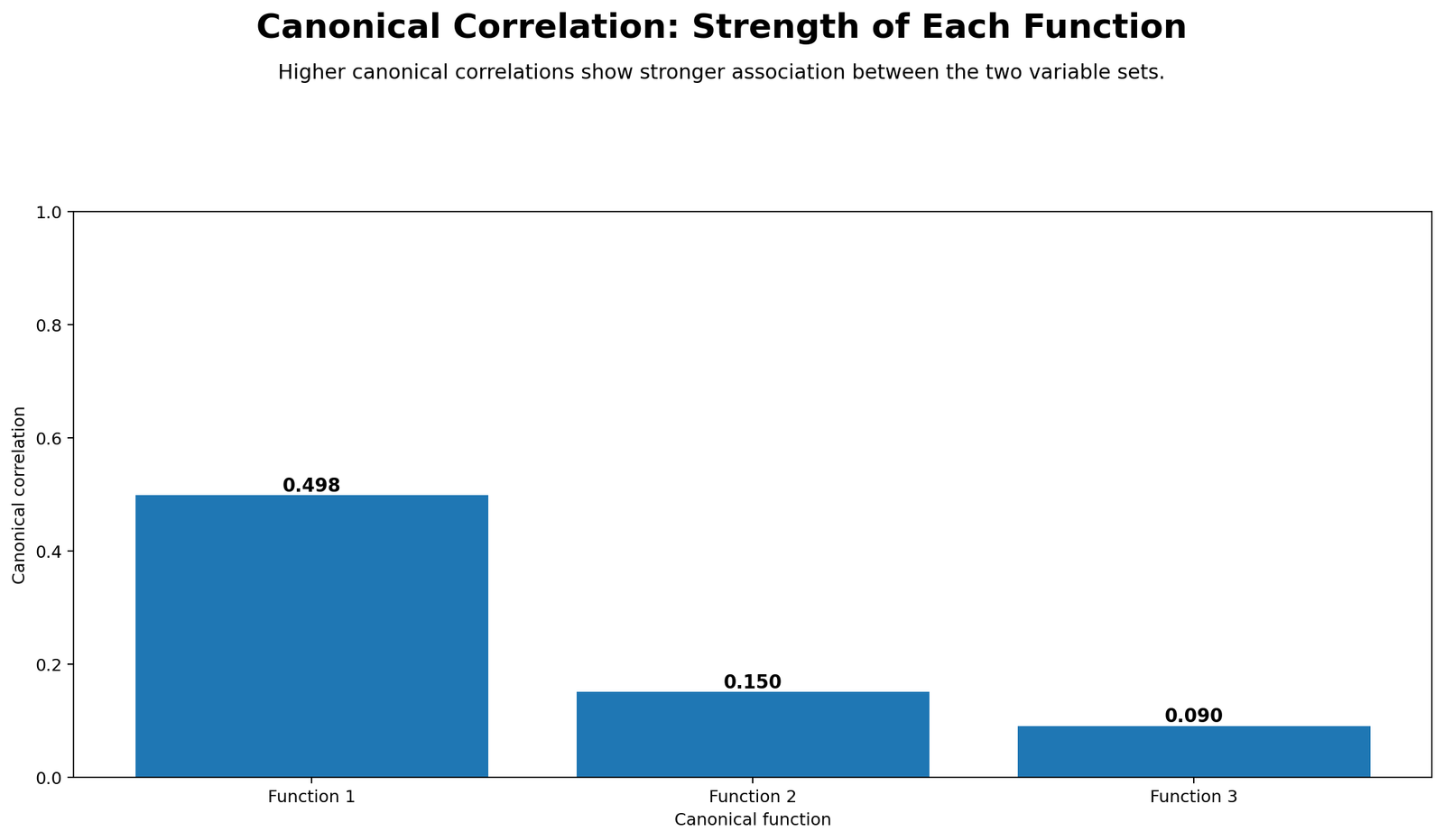
This chart makes the main result easy to see. Function 1 has the largest canonical correlation, about .498. Function 2 drops sharply to about .150, and Function 3 is only about .090. The first bar is therefore the only practically meaningful root in the Python/SPSS setup, even though the dimension test for Function 2 is statistically detectable.
The visual gap between Function 1 and the later functions is important. It shows that the main multivariate relationship is concentrated in the first canonical variate pair. The later functions add very little extra shared variance, so a clear report should emphasize Function 1 and treat the remaining roots as secondary checks.
Python Chart 2: First Canonical Variate Scatterplot
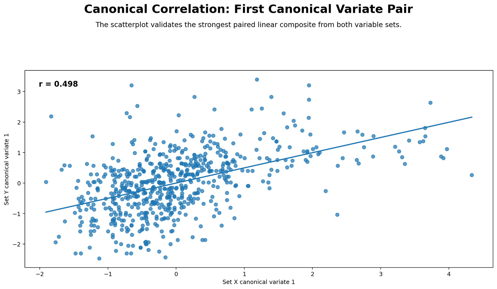
The scatterplot shows each student as a point using the first Set X canonical variate score on the horizontal axis and the first Set Y canonical variate score on the vertical axis. The fitted line slopes upward, matching the displayed r = .498. The cloud is not perfectly tight, but it has a clear positive direction.
This chart validates the first canonical correlation in a way that a table cannot. Most points cluster near the center, while a smaller group extends toward higher canonical scores. The upward trend means that students with higher values on the X-side composite tend to have higher values on the Y-side composite after the weights are applied. The moderate spread around the line explains why the correlation is moderate rather than extremely high.
Python Chart 3: Set X Structure Loadings
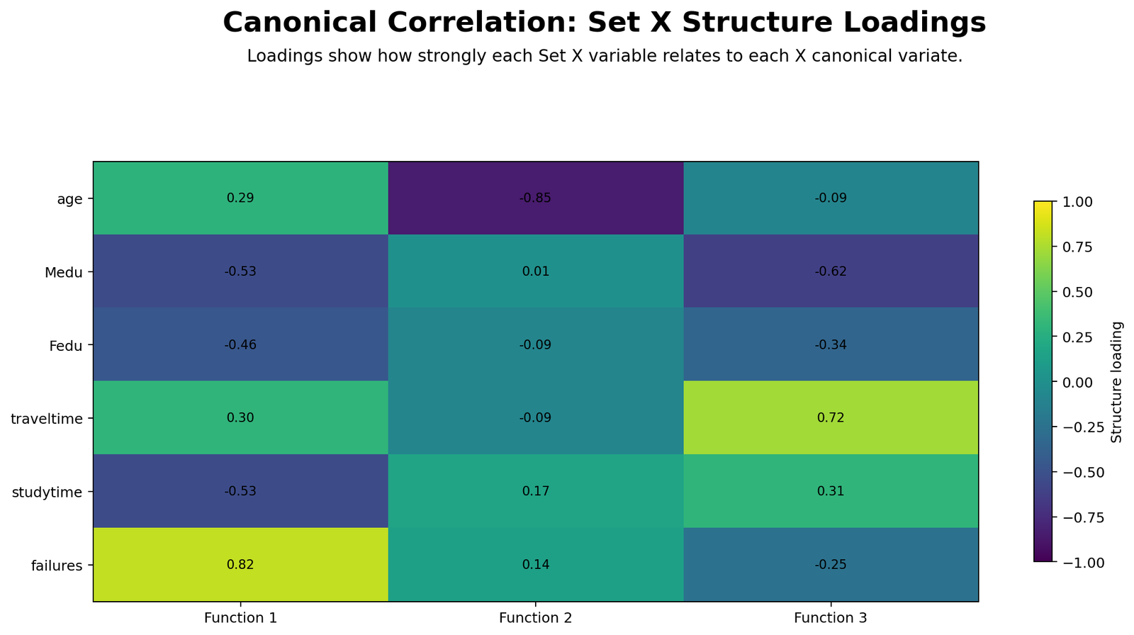
The Set X loading heatmap shows that failures is the dominant Function 1 loading at about .82. studytime and Medu both load around -.53, while Fedu is about -.46. Age and travel time have smaller positive Function 1 loadings, around .29 to .30. This pattern means the first X-side composite is not a simple “all good factors” score; it is a contrast where previous failures sit opposite study time and parental education.
Function 2 is dominated by age with a large negative loading near -.85, while Function 3 is mainly connected with traveltime around .72 and Medu around -.62. Because the later canonical correlations are small, these later loading patterns should not be overinterpreted. The strongest and most useful story remains Function 1.
Python Chart 4: Set Y Structure Loadings
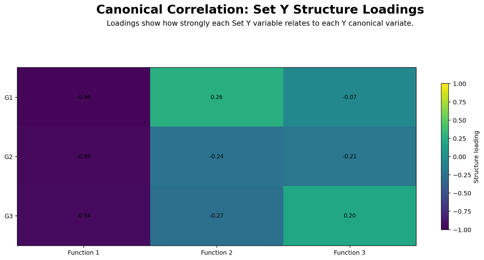
The Set Y heatmap is very clear: G1, G2 and G3 all load strongly and negatively on Function 1, with values around -.96, -.95 and -.94. Because signs in canonical correlation are arbitrary, the negative sign is not the main message. The magnitude is the main message. Function 1 represents a strong general academic-performance composite.
The later functions do not show the same clean grade pattern. Function 2 has smaller values, and Function 3 is weak. This confirms that the first canonical function is the meaningful one for the grade set. In plain words, the Y-side of the first function is “overall grades.”
Python Chart 5: Redundancy Summary
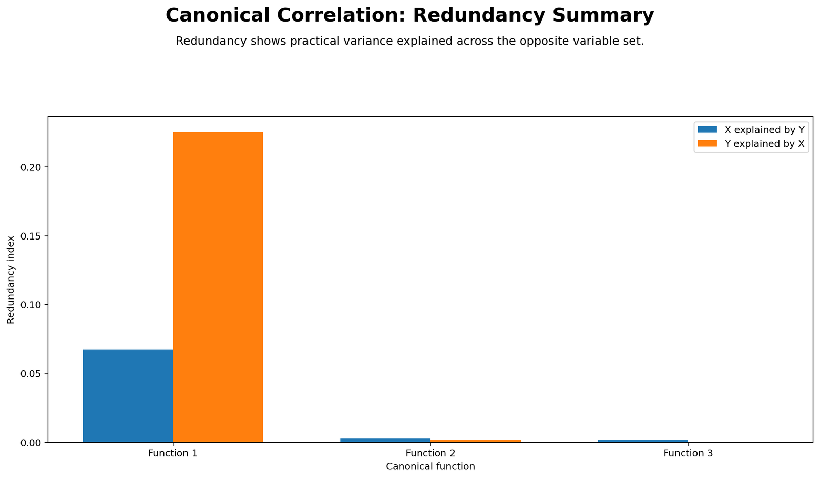
The redundancy chart gives the practical interpretation that raw canonical correlations can hide. Function 1 explains about .225 of the Y set through the X set, while the X set explained by the Y set is much smaller at about .067. In percentage language, the predictor set explains about 22.5% of the grade-set variance through Function 1, while the grade set explains about 6.7% of the predictor-set variance.
Functions 2 and 3 are almost flat in the chart. This tells the reader that the later roots do not add much practical variance explanation. The best report should therefore combine the root chart and redundancy chart: Function 1 is statistically significant and meaningful, but the practical variance explained is more modest than the canonical loading table might initially suggest.
Python Chart 6: Input Correlation Matrix
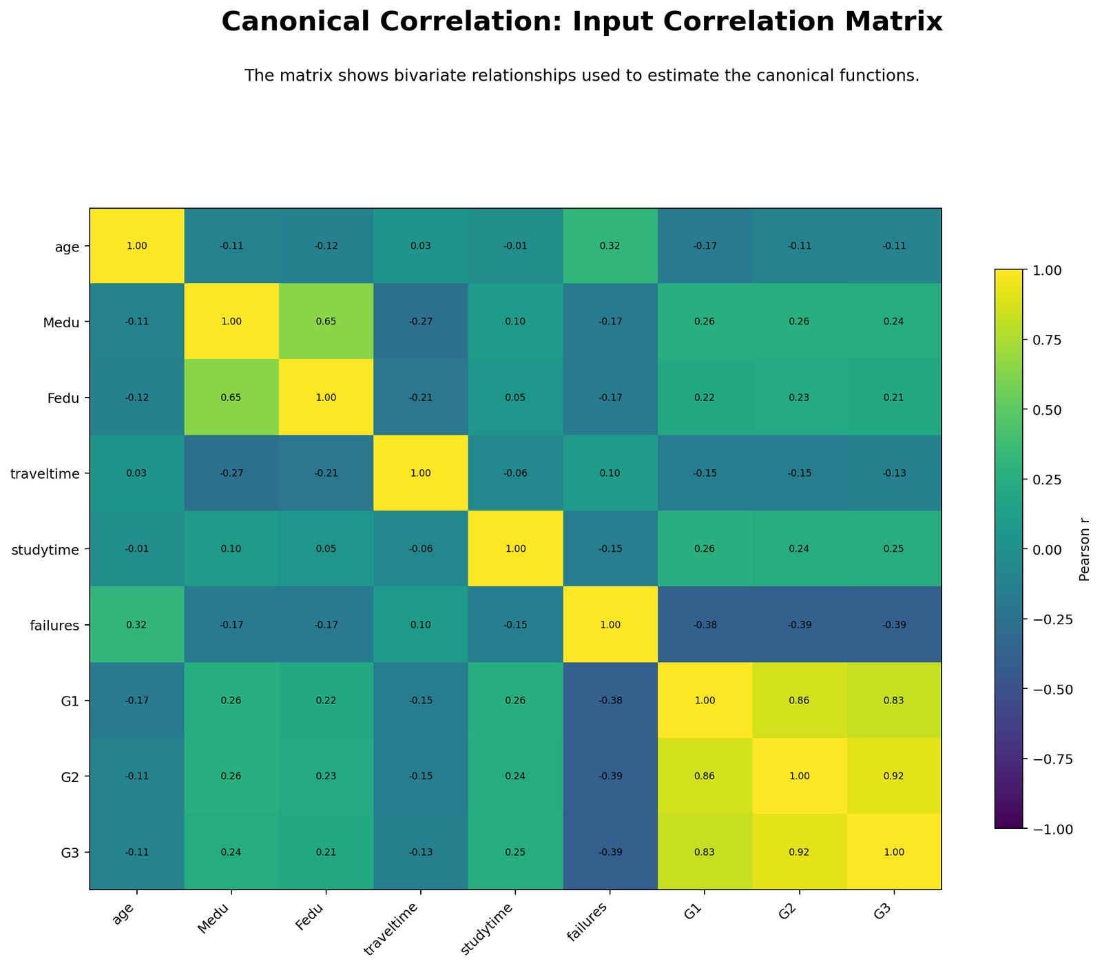
The input matrix explains why the first canonical function is mostly a grade-performance relationship. G1 and G2 correlate about .86, G2 and G3 correlate about .92, and G1 and G3 correlate about .83. These strong grade-to-grade correlations make the Y set highly coherent.
The predictor-side story is more mixed. failures correlates negatively with the grade variables, around -.38 to -.39. studytime correlates positively with grades around .24 to .26. Mother and father education also show positive links with the grade variables. This matrix supports the loading interpretation: failures, studytime and parental education provide the main cross-set connection to academic performance.
R Chart-by-Chart Validation
The R report uses an expanded validation setup. Set 1 contains G1, G2, G3 and absences. Set 2 contains background, study, family, social, alcohol and health variables. Because the R variable sets differ from the Python/SPSS setup, the exact numeric roots are different. The interpretation logic is the same: identify the strongest roots, inspect the scatterplot, read structure loadings and then check redundancy.
R Chart 1: Colorful Root Strength by Function
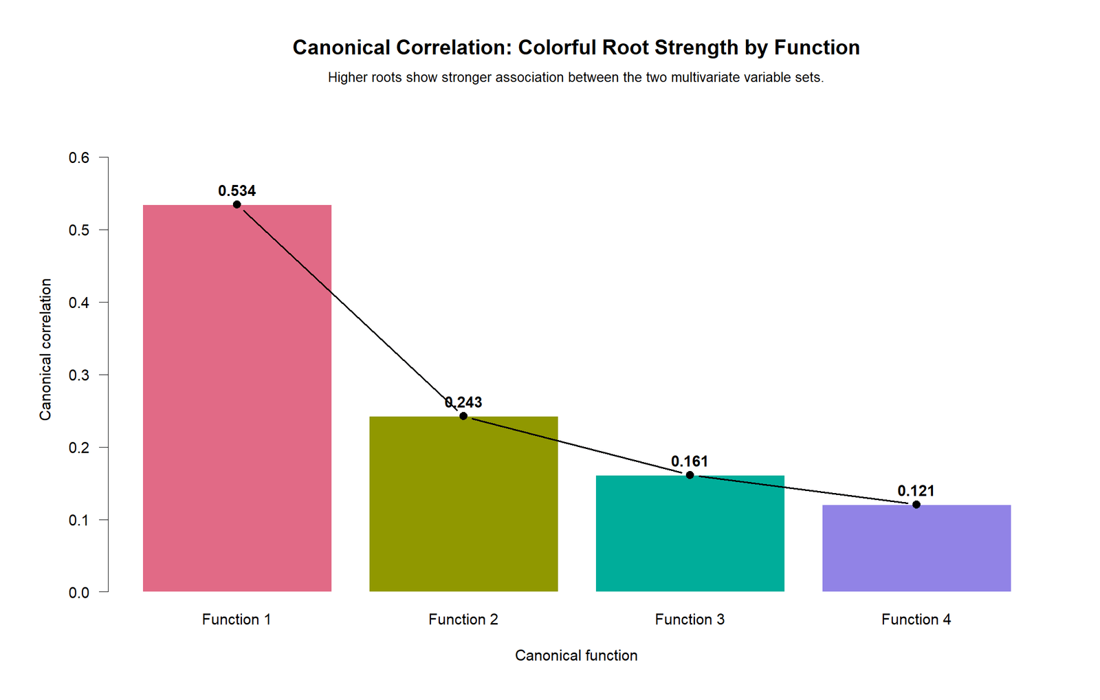
The R root chart shows a larger first function than the Python/SPSS setup because the variable blocks are defined differently. Function 1 is about .534, Function 2 is about .243, Function 3 is about .161, and Function 4 is about .121. The sharp decline after Function 1 again shows that most of the useful relationship sits in the first root.
The R dimension tests support the first two roots but not the last two. However, the first root is still the clearest practical story. The chart’s descending pattern is exactly what a good canonical correlation report should show: interpret the first function strongly, mention the second cautiously if significant, and avoid overexplaining weak residual roots.
R Chart 2: Colorful Function 1 Scores
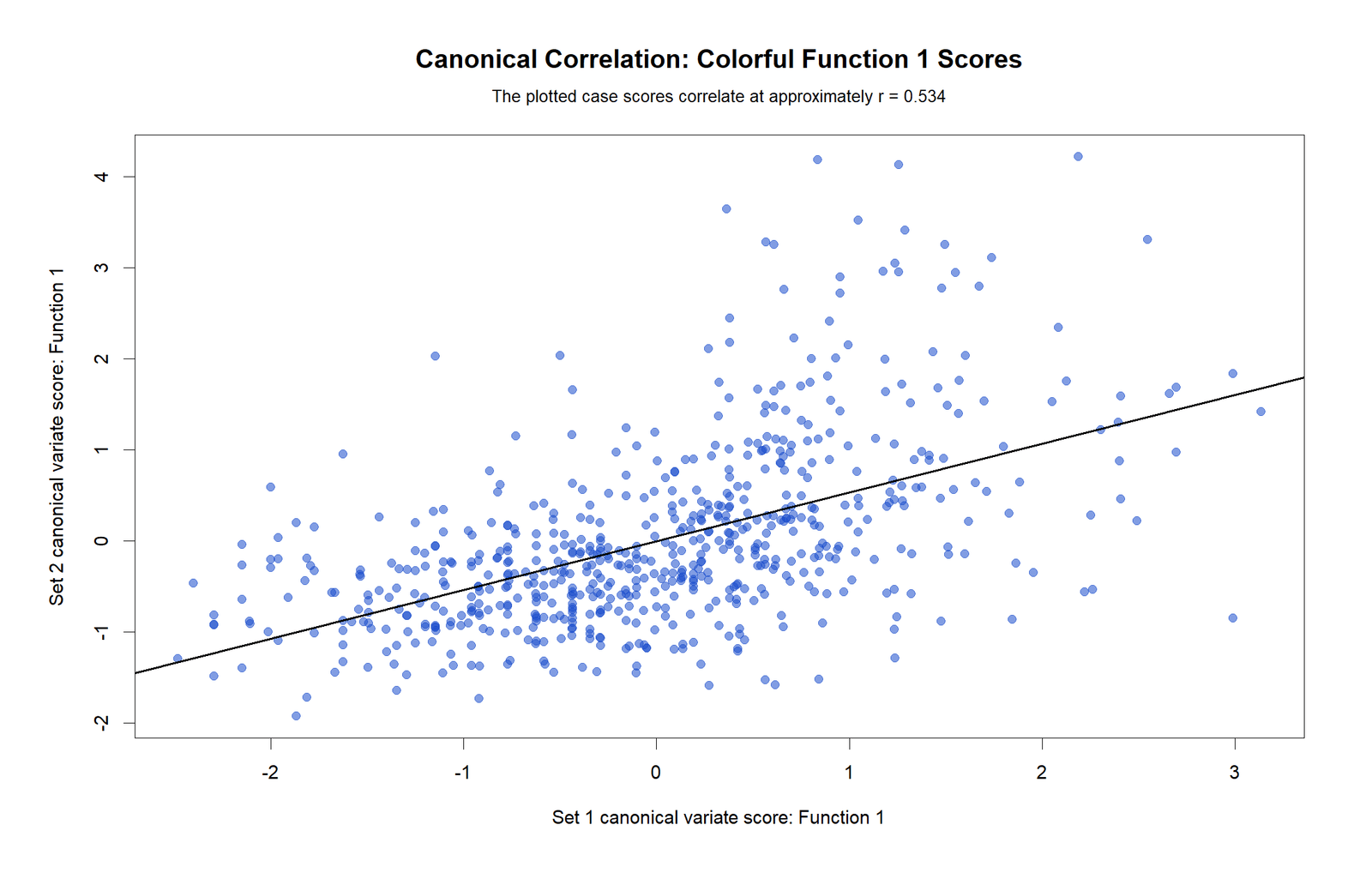
The R scatterplot shows the first canonical variate scores from Set 1 and Set 2. The fitted line slopes upward, and the chart states that the case scores correlate at approximately r = .534. This confirms a moderate positive multivariate relationship in the expanded setup.
The points are spread around the line, so the relationship is not deterministic. The plot shows a general upward tendency rather than perfect separation. That is why the root is meaningful but still moderate. It supports the same reporting style as the Python chart: state the root, then explain the variables driving it through structure loadings.
R Chart 3: Colorful Structure Loadings Heatmap
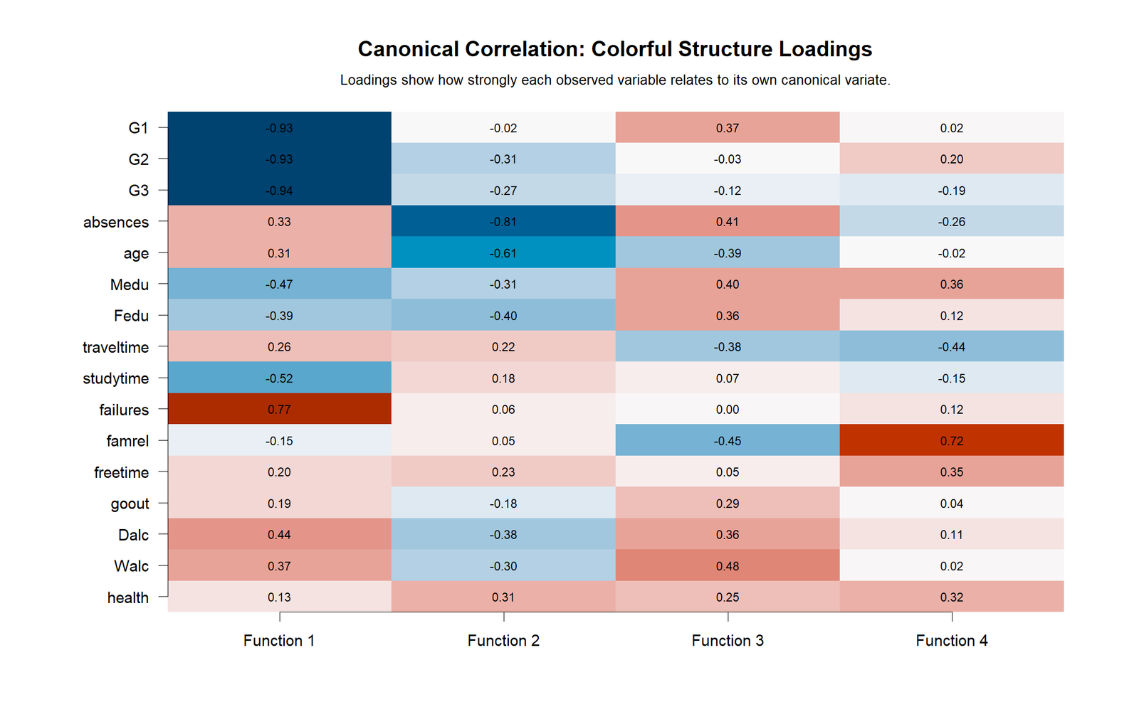
The R loading heatmap shows that Function 1 is strongly tied to grades on the Set 1 side: G1 = -.93, G2 = -.93 and G3 = -.94. Absences is much smaller at about .33. On the Set 2 side, failures has a strong loading around .77, while studytime is around -.52, Medu around -.47, and alcohol variables show positive moderate loadings.
This chart gives the substantive meaning of the first function. It is mainly an academic-performance dimension linked with prior failures, study time, parental education and some lifestyle indicators. The later functions show different patterns, such as absences loading strongly on Function 2 and family relationship loading strongly on Function 4, but those functions have weaker roots and should be interpreted cautiously.
R Chart 4: Colorful Function 1 Standardized Coefficients
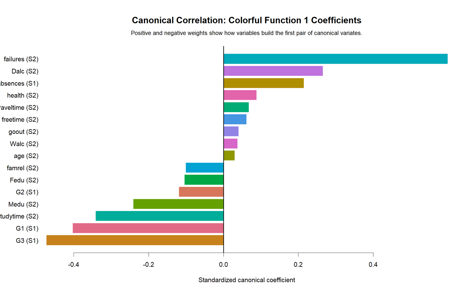
The R coefficient chart shows which variables receive the largest standardized weights in Function 1. failures has a large positive weight, while G3 and G1 have large negative weights. Studytime and Medu also appear with negative weights. This coefficient pattern is consistent with the loading pattern: academic performance is contrasted with previous failures and related background-study characteristics.
Coefficients should be read carefully because they can change when variables are highly correlated. In this data, G1, G2 and G3 are strongly related to one another, so structure loadings are often more stable for interpretation than raw weights. The coefficient chart is useful, but it should not replace the loading heatmap.
R Chart 5: Colorful Redundancy by Function
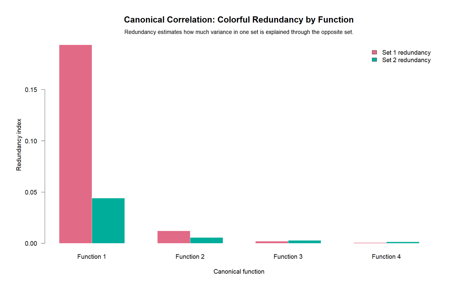
The R redundancy chart shows that Function 1 carries almost all of the practical explanation. Set 1 redundancy for Function 1 is about .194, while Set 2 redundancy is about .044. The later functions are very small, with Function 2 only around .012 for Set 1 and .006 for Set 2.
This chart is the practical check on the root chart. A root can be statistically significant but still explain little practical variance in the opposite set. The R redundancy plot confirms that the article should focus on Function 1 and avoid presenting the weaker roots as equally important.
Excel Results Explained
The Excel workbook gives a fully worked formula-based version of canonical correlation. It uses a compact 2 by 2 setup so the matrix method can be shown transparently using Excel formulas such as CORREL, MINVERSE and MMULT. The Excel variable sets are different from the main Python/SPSS report: X set = G1 and G2, while Y set = G3 and absences.
Excel Worked Example: G1 and G2 Against G3 and Absences
| Excel Item | Value | Interpretation |
|---|---|---|
| Complete cases | 649 | All complete student records were used. |
| X set | G1, G2 | Earlier grade variables form the first block. |
| Y set | G3, absences | Final grade and absences form the second block. |
| Maximum roots | 2 | The smaller set contains two variables, so Excel returns two functions. |
| Function 1 eigenvalue | 0.849880 | This is the squared first canonical correlation. |
| Function 1 canonical r | 0.921889 | Very strong first canonical relationship. |
| Function 1 r squared | 0.849880 | The first canonical variates share about 84.99% variance. |
| Function 1 Wilks Lambda | 0.149392 | Low Lambda indicates a strong multivariate relationship remains. |
| Function 1 chi-square | 1227.213 | Bartlett approximation strongly rejects no relationship. |
| Function 1 p-value | ≈ 2.01 × 10-264 | The first function is decisively significant. |
| Function 2 canonical r | 0.069629 | Very weak leftover relationship. |
| Function 2 p-value | 0.07653 | Not significant at alpha .05. |
The Excel result is very strong because G1 and G2 are highly connected to G3. In the workbook, G1 correlates with G3 at about .826, G2 correlates with G3 at about .919, and G1 correlates with G2 at about .865. Absences has weaker negative relationships with the grade variables, including about -.147 with G1, -.125 with G2 and -.091 with G3. This means the first Excel canonical variate is mainly a grade-to-grade relationship, not an absence-driven relationship.
The workbook also shows the exact matrix path. First, Excel builds Rxx, Ryy and Rxy using CORREL. Then it creates M = Rxx-1 Rxy Ryy-1 Ryx using MINVERSE and MMULT. Because the matrix is 2 by 2, the workbook uses the quadratic eigenvalue formula to calculate the two roots. Function 1 is strong and significant; Function 2 is weak and not significant.
Excel interpretation rule: The Excel workbook should be described as a transparent worked example, not as a replacement for the main SPSS/Python variable-set result. It answers a smaller formula-learning question: how do we calculate canonical correlation manually in Excel for two variables in each set?
Excel Formula Steps Used in the Workbook
| Step | Excel Formula Pattern | Purpose |
|---|---|---|
| Build Rxx | =CORREL(G1_range,G2_range) | Calculate within-set correlations for X variables. |
| Build Ryy | =CORREL(G3_range,absences_range) | Calculate within-set correlations for Y variables. |
| Build Rxy | =CORREL(X_variable,Y_variable) | Calculate cross-set correlations. |
| Invert matrices | =MINVERSE(Rxx_range) | Create inverse correlation matrices. |
| Create root matrix | =MMULT(MMULT(MINVERSE(Rxx),Rxy),MMULT(MINVERSE(Ryy),TRANSPOSE(Rxy))) | Build the canonical root matrix. |
| Eigenvalue 1 | =((M11+M22)+SQRT((M11-M22)^2+4*M12*M21))/2 | Calculate the larger 2 by 2 matrix eigenvalue. |
| Canonical r | =SQRT(eigenvalue) | Convert each eigenvalue to a canonical correlation. |
| Wilks Lambda | =PRODUCT(1-lambda_i) | Calculate the remaining unexplained multivariate proportion. |
| p-value | =CHISQ.DIST.RT(chi_square,df) | Test significance using Bartlett’s chi-square approximation. |
SPSS, R, Python and Excel Workflows for Canonical Correlation
The same canonical-correlation logic can be reproduced in SPSS, R, Python and Excel. The key is to define the two variable sets first. If the variable sets change, the canonical correlations, roots, redundancy and loadings will also change.
| Software | Main Steps | Best Use |
|---|---|---|
| SPSS | Use MANOVA /DISCRIM or syntax-based canonical correlation; inspect roots, Wilks Lambda, standardized coefficients, structure correlations and redundancy. | Formal output PDF, thesis reporting and classroom verification. |
| Python | Use pandas and numpy to standardize variables, build correlation matrices, solve eigenvalues, calculate Wilks Lambda and create charts. | Automated chart production, reproducible calculations and custom reports. |
| R | Use cancor(), correlation matrices, structure loadings, Bartlett tests and redundancy calculations. | Statistical validation and flexible publication-ready visuals. |
| Excel | Use CORREL, MINVERSE, MMULT, TRANSPOSE, SQRT and CHISQ.DIST.RT. | Step-by-step formula teaching and fully worked manual calculation. |
Code Blocks for Canonical Correlation
SPSS Syntax for Canonical Correlation
* Canonical Correlation Analysis in SPSS.
* Set X covariates: age Medu Fedu traveltime studytime failures.
* Set Y dependent variables: G1 G2 G3.

OUTPUT CLOSE ALL.
OUTPUT NEW NAME=Canonical_Correlation_Output.

TITLE "Canonical Correlation Analysis".

MANOVA G1 G2 G3 WITH age Medu Fedu traveltime studytime failures
  /DISCRIM ALL ALPHA(1)
  /PRINT SIGNIF(EIGEN DIMENR) PARAM(ESTIM)
  /ANALYSIS G1 G2 G3 WITH age Medu Fedu traveltime studytime failures
  /DESIGN.

CORRELATIONS
  /VARIABLES=age Medu Fedu traveltime studytime failures G1 G2 G3
  /PRINT=TWOTAIL
  /MISSING=PAIRWISE.

DESCRIPTIVES VARIABLES=age Medu Fedu traveltime studytime failures G1 G2 G3
  /STATISTICS=MEAN STDDEV MIN MAX.

OUTPUT EXPORT
  /CONTENTS EXPORT=VISIBLE
  /PDF DOCUMENTFILE='Canonical-Correlation-SPSS-Output.pdf'.
Python Code for Canonical Correlation
import pandas as pd
import numpy as np
from scipy.stats import chi2

# Load data
df = pd.read_csv("dataset.csv")

x_vars = ["age", "Medu", "Fedu", "traveltime", "studytime", "failures"]
y_vars = ["G1", "G2", "G3"]

work = df[x_vars + y_vars].apply(pd.to_numeric, errors="coerce").dropna()
X = work[x_vars].to_numpy()
Y = work[y_vars].to_numpy()

# Standardize variables
Xz = (X - X.mean(axis=0)) / X.std(axis=0, ddof=1)
Yz = (Y - Y.mean(axis=0)) / Y.std(axis=0, ddof=1)

# Correlation matrices
Z = np.column_stack([Xz, Yz])
R = np.corrcoef(Z, rowvar=False)
p = len(x_vars)
q = len(y_vars)
Rxx = R[:p, :p]
Ryy = R[p:, p:]
Rxy = R[:p, p:]
Ryx = Rxy.T

# Canonical root matrix and roots
M = np.linalg.inv(Rxx) @ Rxy @ np.linalg.inv(Ryy) @ Ryx
eigenvalues = np.real(np.linalg.eigvals(M))
eigenvalues = np.sort(eigenvalues)[::-1]
eigenvalues = eigenvalues[:min(p, q)]
canonical_r = np.sqrt(np.maximum(eigenvalues, 0))

print("Canonical correlations:", canonical_r)
print("Squared canonical correlations:", canonical_r ** 2)

# Wilks Lambda sequential tests using Bartlett approximation
n = len(work)
for i in range(len(eigenvalues)):
    remaining = eigenvalues[i:]
    wilks = np.prod(1 - remaining)
    df_test = (p - i) * (q - i)
    chi_square = -(n - 1 - (p + q + 1) / 2) * np.log(wilks)
    p_value = chi2.sf(chi_square, df_test)
    print(i + 1, "to", len(eigenvalues), "Wilks", wilks,
          "Chi-square", chi_square, "df", df_test, "p", p_value)
R Code for Canonical Correlation
# Canonical Correlation Analysis in R

df <- read.csv("dataset.csv")

x_vars <- c("age", "Medu", "Fedu", "traveltime", "studytime", "failures")
y_vars <- c("G1", "G2", "G3")

work <- na.omit(df[, c(x_vars, y_vars)])
work[] <- lapply(work, as.numeric)

X <- scale(work[, x_vars])
Y <- scale(work[, y_vars])

cca <- cancor(X, Y)
print(cca$cor)
print(cca$xcoef)
print(cca$ycoef)

# Canonical scores
U <- as.matrix(X) %*% cca$xcoef
V <- as.matrix(Y) %*% cca$ycoef

# Structure loadings
x_loadings <- cor(X, U)
y_loadings <- cor(Y, V)
print(x_loadings)
print(y_loadings)

# Redundancy approximation
r2 <- cca$cor^2
x_variance_extracted <- colMeans(x_loadings^2)
y_variance_extracted <- colMeans(y_loadings^2)
x_redundancy <- x_variance_extracted * r2
y_redundancy <- y_variance_extracted * r2
print(data.frame(r = cca$cor, r2 = r2,
                 x_variance_extracted = x_variance_extracted,
                 y_variance_extracted = y_variance_extracted,
                 x_redundancy = x_redundancy,
                 y_redundancy = y_redundancy))
Excel Formulas for Canonical Correlation
Step 1: Build the within-set correlation matrices.
=CORREL(X1_range, X2_range)
=CORREL(Y1_range, Y2_range)

Step 2: Build the cross-set correlation matrix.
=CORREL(X1_range, Y1_range)
=CORREL(X1_range, Y2_range)
=CORREL(X2_range, Y1_range)
=CORREL(X2_range, Y2_range)

Step 3: Create the canonical root matrix.
=MMULT(MMULT(MINVERSE(Rxx), Rxy), MMULT(MINVERSE(Ryy), TRANSPOSE(Rxy)))

Step 4: For a 2 by 2 matrix M, calculate eigenvalues.
=((M11+M22)+SQRT((M11-M22)^2+4*M12*M21))/2
=((M11+M22)-SQRT((M11-M22)^2+4*M12*M21))/2

Step 5: Convert eigenvalues into canonical correlations.
=SQRT(eigenvalue)

Step 6: Calculate Wilks Lambda.
=PRODUCT(1-lambda_i)

Step 7: Calculate p-value from Bartlett chi-square approximation.
=CHISQ.DIST.RT(chi_square, df)
APA Reporting Wording for Canonical Correlation
When reporting Canonical Correlation Analysis, describe the two variable sets, sample size, number of functions, canonical correlations, Wilks Lambda dimension tests, main structure loadings, redundancy results and the practical interpretation. Also state clearly which functions are interpreted and which are not.
APA-Style Full Report
A canonical correlation analysis was conducted to examine the multivariate association between a background/study predictor set and an academic grade outcome set. Set X contained age, mother education, father education, travel time, study time and past failures. Set Y contained G1, G2 and G3. The analysis included 649 complete cases. The first canonical function was statistically significant, Wilks Lambda = .729, F(18, 1810.68) = 11.91, p < .001, with a canonical correlation of rc = .498 and squared canonical correlation of .248. The second function was statistically significant but weak, rc = .150, p = .030, while the third function was not significant, rc = .090, p = .260. Function 1 was primarily defined by failures, study time and parental education in the predictor set and by strong loadings for G1, G2 and G3 in the grade set. Redundancy results showed that the predictor set explained about 22.5% of the grade-set variance through Function 1.
Short APA-Style Version
Canonical correlation analysis showed a significant relationship between the background/study predictor set and the grade outcome set, Wilks Lambda = .729, p < .001. The first canonical function was moderate, rc = .498, rc2 = .248, and was mainly defined by failures, study time, parental education and the grade variables G1, G2 and G3. Later functions were much weaker and were not emphasized in interpretation.
Excel Worked-Example Wording
For the Excel formula demonstration, canonical correlation was calculated between X set (G1 and G2) and Y set (G3 and absences). The first canonical function was very strong, rc = .9219, rc2 = .8499, Wilks Lambda = .1494, chi-square = 1227.21, p < .001. The second function was weak and not significant, rc = .0696, p = .0765. This Excel result is a compact formula example and uses different variable sets from the main SPSS/Python report.
Common Mistakes in Canonical Correlation Interpretation
| Mistake | Why It Is a Problem | Better Practice |
|---|---|---|
| Interpreting every canonical root equally | Later roots can be statistically small or not significant. | Use Wilks Lambda tests, root size and redundancy to decide which functions matter. |
| Ignoring variable-set definitions | Changing the variables in Set X or Set Y changes the result. | State both sets clearly before reporting coefficients. |
| Reporting only canonical r | A high root can still have limited practical redundancy. | Report r, r squared, structure loadings and redundancy indices. |
| Overusing canonical weights | Weights can be unstable under multicollinearity. | Prefer structure loadings for substantive interpretation. |
| Treating signs as fixed | Canonical signs can reverse without changing the relationship. | Focus on magnitude and pattern; describe sign direction carefully. |
| Ignoring multicollinearity | Highly correlated variables can distort coefficients and weights. | Check correlation matrices, VIF and tolerance where appropriate. |
| Mixing results from different variable sets | Python, R and Excel examples may use different blocks. | Explain when a workbook or validation run uses a different teaching setup. |
When to Use Canonical Correlation
Use Canonical Correlation Analysis when you have two meaningful sets of continuous or approximately continuous variables and you want to understand the multivariate relationship between those sets. It is useful when many separate correlations would be confusing and when the research question is naturally set-based.
Good examples include study habits and grade outcomes, psychological scales and health measures, customer behavior metrics and business performance indicators, socioeconomic variables and educational outcomes, or multiple predictors and multiple responses. If you have one outcome and many predictors, multiple linear regression may be better. If you have group differences across multiple outcomes, MANOVA may be more appropriate. If you want to reduce variables within one set, principal component analysis may be the better first tool.
Downloads and Resources for Canonical Correlation
R Canonical Correlation Report PDFIncludes R validation charts, roots, loadings, coefficients and redundancy indices.
SPSS Canonical Correlation Output PDFFormal SPSS output with roots, Wilks Lambda, standardized coefficients and structure correlations.
Excel Fully Worked FileFormula-based Excel workbook showing Rxx, Ryy, Rxy, eigenvalues, canonical roots and Wilks Lambda.
FAQs About Canonical Correlation
What is canonical correlation in simple words?
Canonical correlation measures the strongest relationship between two weighted sets of variables. It creates one composite score from each set and then correlates those composites.
What is a canonical variate?
A canonical variate is a weighted linear combination of variables from one set. In each function, one variate is created from Set X and one variate is created from Set Y.
How do I interpret the first canonical correlation?
The first canonical correlation is the strongest possible correlation between the two variable sets. Interpret it with squared canonical correlation, Wilks Lambda, structure loadings and redundancy.
What does Wilks Lambda mean in canonical correlation?
Wilks Lambda tests whether remaining canonical functions still contain a significant relationship. Smaller values indicate stronger multivariate association.
What are structure loadings?
Structure loadings are correlations between original variables and their own canonical variates. They are often easier to interpret than canonical weights.
What is redundancy in canonical correlation?
Redundancy estimates how much variance in one variable set is explained through the canonical variate from the opposite set. It is a practical effect-size check.
Why are the Python, R and Excel canonical correlations different?
The variable sets are different. Python/SPSS use background and study predictors against G1, G2 and G3. R uses an expanded validation setup. Excel uses a compact 2 by 2 formula example with G1, G2 against G3 and absences.
Can I calculate canonical correlation in Excel?
Yes. For a small 2 by 2 example, Excel can calculate the correlation matrices, inverse matrices, root matrix, eigenvalues, canonical correlations and Wilks Lambda using formulas.

