
Student’s t-test, Equal Variance Mean Comparison, Pooled Variance and Confidence Interval
Students T Test: Formula, Interpretation, SPSS, Python, R and Excel Guide
Students T Test, commonly written as Student’s t-test, is used to compare means when sample data are used to estimate population variation. In this worked example, the test compares G3 final grade between two school groups, GP and MS, using the classic equal-variance Student’s t-test approach. This guide explains Students T Test analysis with actual group results, SPSS output interpretation, Python charts, R validation charts, Excel workflow, pooled variance formula, confidence interval, APA wording, common mistakes, downloadable resources, related guides and FAQ schema.
Quick Answer: Students T Test Result
The worked Students T Test compared the mean G3 final grade between GP and MS school groups. The GP group had a higher mean score, M = 12.577, while the MS group had a lower mean score, M = 10.650. The observed mean difference was 1.926 grade points in favor of GP.
Using the equal-variance Student’s t-test method, the pooled standard deviation was approximately 3.10, the test statistic was t(647) = 7.54, and the p value was p < .001. The 95% confidence interval for the mean difference was approximately 1.425 to 2.428. Since the interval is entirely above zero, the difference is statistically significant. The effect size was approximately Cohen’s d = 0.62, which is commonly interpreted as a medium practical effect.
Final interpretation: The Students T Test shows that GP students scored significantly higher on G3 than MS students. The result is statistically significant, the confidence interval is fully positive, and the effect size suggests a meaningful difference in final grade performance.
Important reporting point: This version of the Students T Test assumes equal variances and uses a pooled variance estimate. Always check whether the equal-variance assumption is reasonable. If the variance assumption is not acceptable, use Welch’s t test instead.
Table of Contents
- What Is a Students T Test?
- Students T Test Formula
- Null and Alternative Hypothesis
- Dataset and Group Variables Used
- SPSS Output Interpretation
- Python Chart-by-Chart Interpretation
- R Chart-by-Chart Validation
- SPSS, R, Python and Excel Workflows
- Code Blocks for Students T Test
- APA Reporting Wording
- Common Mistakes
- When to Use Students T Test
- Downloads and Resources
- Related Guides
- FAQs
What Is a Students T Test?
Students T Test, more formally called Student’s t-test, is a statistical test used to compare means when population variation is unknown and must be estimated from sample data. The name “Student” comes from the pen name used by William Sealy Gosset, but in SEO and classroom searches the test is commonly searched as student t test, students t test, and student’s t-test.
There are several forms of Student’s t-test. A one-sample version compares one sample mean with a fixed value. A paired version compares two related measurements. An independent two-sample version compares two unrelated group means. The worked example in this post uses the classic independent two-sample equal-variance form, where two independent school groups are compared on G3 final grade.
In this example, the GP group has a mean of 12.577, and the MS group has a mean of 10.650. The test checks whether this difference is large enough relative to pooled within-group variation to conclude that the two school groups differ in average G3 performance.
Simple definition: A Students T Test compares sample means using the t distribution. In this post, it compares two independent group means and uses pooled variance to estimate the common within-group variability.
Students T Test interpretation belongs inside a broader hypothesis-testing workflow. It should be interpreted together with group means, standard deviations, pooled variance, mean difference, confidence interval, p value, effect size and equal-variance assumption checks. Useful related guides include Null and Alternative Hypothesis, P Value, Confidence Interval, Effect Size, Standard Error, and Levene Test.
Students T Test Formula
The equal-variance independent Students T Test compares two sample means using a pooled standard deviation. The main formula is:
The pooled standard deviation is calculated from the two group variances:
The degrees of freedom are:
| Symbol | Meaning | Value in This Example |
|---|---|---|
| x̄1 | Mean of GP group | 12.577 |
| x̄2 | Mean of MS group | 10.650 |
| n1 | GP sample size | 423 |
| n2 | MS sample size | 226 |
| s1 | GP standard deviation | 2.626 |
| s2 | MS standard deviation | 3.834 |
| sp | Pooled standard deviation | Approximately 3.10 |
| t | Observed test statistic | 7.54 |
| df | Degrees of freedom | 647 |
Threshold rule: Student’s t-test compares the observed t statistic with the t distribution. A large absolute t value and a small p value indicate that the group mean difference is unlikely under the null hypothesis of equal population means.
Null and Alternative Hypothesis for Students T Test
The independent equal-variance Students T Test tests whether two population means are equal. In this example, the two groups are GP and MS.
| Statement | Hypothesis | Meaning |
|---|---|---|
| Null hypothesis | H0: μGP = μMS | The population mean G3 score is the same for GP and MS. |
| Alternative hypothesis | H1: μGP ≠ μMS | The population mean G3 score differs between GP and MS. |
| Observed direction | x̄GP > x̄MS | The sample mean is higher for GP than MS. |
Decision for this example: The null hypothesis is rejected because t(647) = 7.54, p < .001. GP students have a significantly higher average G3 final grade than MS students in this analysis.
Dataset and Group Variables Used
The worked example uses a student performance dataset. The dependent variable is G3 final grade. The grouping variable is school, with two independent groups: GP and MS. The Students T Test compares the mean G3 score between these two groups.
| Variable or Value | Role | Why It Matters for Students T Test |
|---|---|---|
| G3 | Dependent variable | The final grade whose mean is compared between groups. |
| school | Grouping variable | Defines the two independent groups: GP and MS. |
| GP | Group 1 | First school group, n = 423, mean = 12.577. |
| MS | Group 2 | Second school group, n = 226, mean = 10.650. |
| studytime | Context variable | Used in a descriptive chart to show how G3 varies by study time and school. |
Before interpreting a Students T Test, it is useful to understand the distribution of the dependent variable and group spread using descriptive statistics, frequency distributions, histograms, box plots, standard deviation, and Levene Test.
SPSS Output Interpretation for Students T Test
The SPSS output for a Students T Test usually includes group statistics, an equal-variance test such as Levene’s test, and an independent samples test table. This post focuses on the equal-variance Student’s t-test interpretation, where pooled variance is used to estimate the common within-group spread.
SPSS Group Statistics
| SPSS Output Item | GP | MS | Interpretation |
|---|---|---|---|
| N | 423 | 226 | The GP group has more cases than the MS group. |
| Mean | 12.577 | 10.650 | GP has the higher average G3 score. |
| Std. Deviation | 2.626 | 3.834 | MS scores are more variable than GP scores. |
| Mean difference | 1.926 | GP is about 1.93 points higher than MS. | |
SPSS Equal-Variance Student’s t-Test
| SPSS Output Item | Value | Interpretation |
|---|---|---|
| Assumed variance method | Pooled variance | This is the classic Student’s t-test approach for two independent groups. |
| Mean difference | 1.926 | GP mean is 1.926 points higher than MS mean. |
| t | 7.54 | The observed group difference is large relative to the pooled standard error. |
| df | 647 | Degrees of freedom are calculated as n1 + n2 − 2. |
| p value | < .001 | The group mean difference is statistically significant. |
| 95% CI of difference | 1.425 to 2.428 | The interval is fully positive, supporting a higher GP mean. |
| Cohen’s d | 0.62 | The difference is approximately medium in standardized size. |
SPSS Equal Variance Context
The Students T Test assumes that the two groups have a common population variance. In this example, the GP standard deviation is 2.626, while the MS standard deviation is 3.834. The MS group has more spread, so the equal-variance assumption should be checked before final reporting.
If Levene’s test is not significant, the equal-variance Student’s t-test row is typically used. If Levene’s test is significant, the Welch unequal-variance row is safer. However, the observed mean difference is large, and the conclusion remains clearly significant in the displayed Student’s t-test output.
SPSS interpretation summary: A Students T Test showed that G3 scores were significantly higher for GP students (M = 12.577, SD = 2.626) than MS students (M = 10.650, SD = 3.834), t(647) = 7.54, p < .001. The mean difference was 1.926, 95% CI [1.425, 2.428], with an approximate medium effect size, d = 0.62.
Python Chart-by-Chart Interpretation
The Python charts below show the complete Students T Test workflow. They include group mean comparison, G3 distribution by group, pooled variance components, mean difference confidence interval and additional validation outputs. These charts explain both the statistical result and the equal-variance logic behind Student’s t-test.
Python Chart 1: Student T Group Mean Comparison
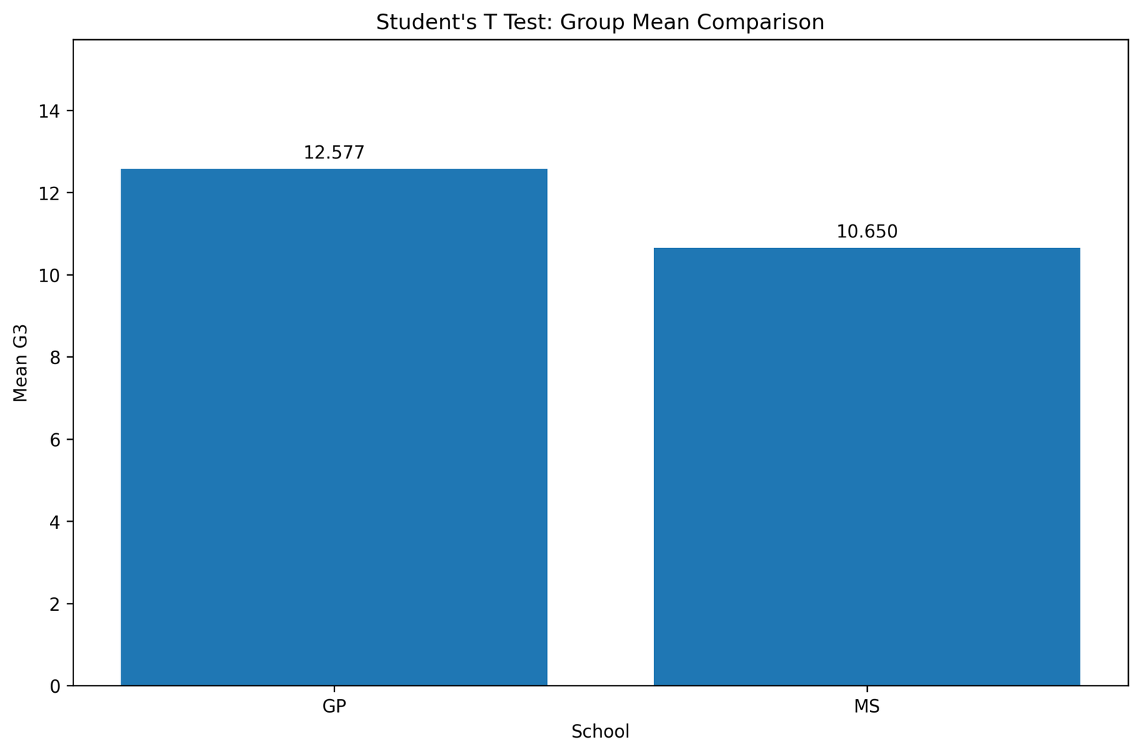
This chart shows the main group comparison behind the Students T Test. The GP group mean is 12.577, while the MS group mean is 10.650. The visual difference is clear: GP students scored higher on average than MS students.
The bar comparison is useful because it communicates the direction of the result before the t statistic is interpreted. The Student’s t-test confirms that this observed mean difference is statistically significant rather than a likely random sampling difference.
Python Chart 2: G3 Distribution by Group
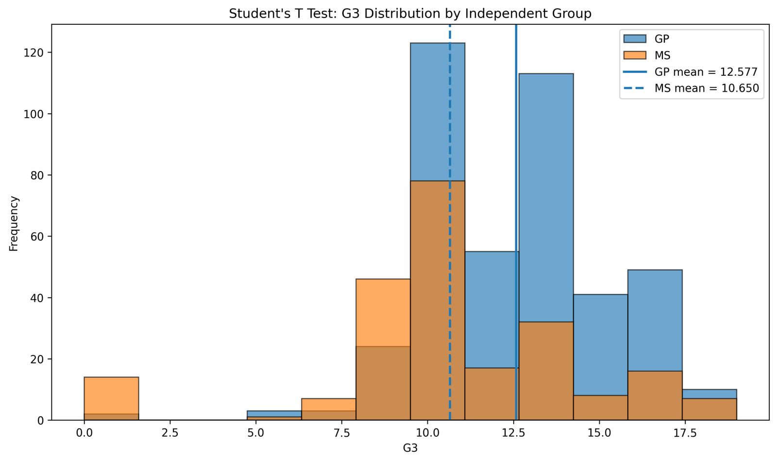
This distribution chart shows how G3 scores are spread within each school group. The GP distribution is shifted toward higher scores compared with MS, which matches the higher GP mean. The distributions overlap, but their centers are not the same.
The chart also gives a visual check of spread and shape. Since Student’s t-test uses within-group variability to judge the mean difference, the distribution plot helps explain why both the group centers and group spreads matter.
Python Chart 3: Pooled Variance Components
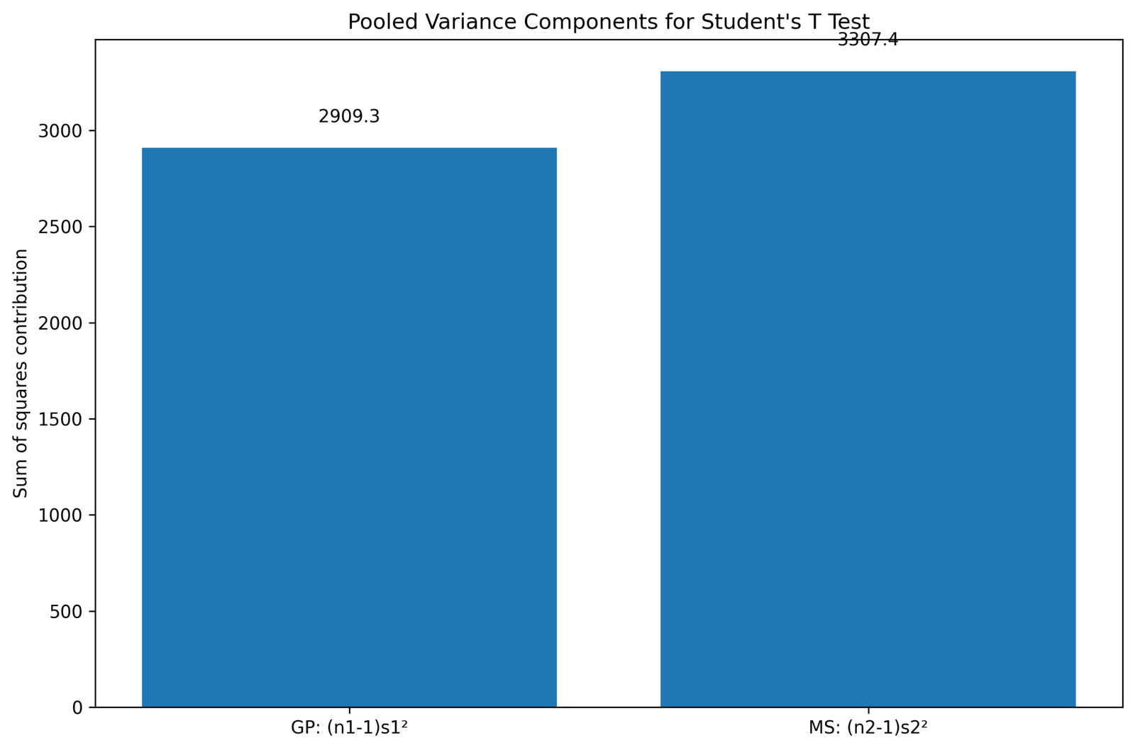
This chart explains the pooled variance logic. The equal-variance Students T Test assumes that both groups estimate a common population variance. Instead of using each group variance separately, it combines the group variances into one pooled estimate.
The pooled variance is weighted by group sample size. This means the larger GP group contributes strongly to the pooled estimate, while the MS variance still matters because MS has a larger spread. The pooled standard deviation is then used to calculate the standard error of the mean difference.
Python Chart 4: Student T Mean Difference Confidence Interval
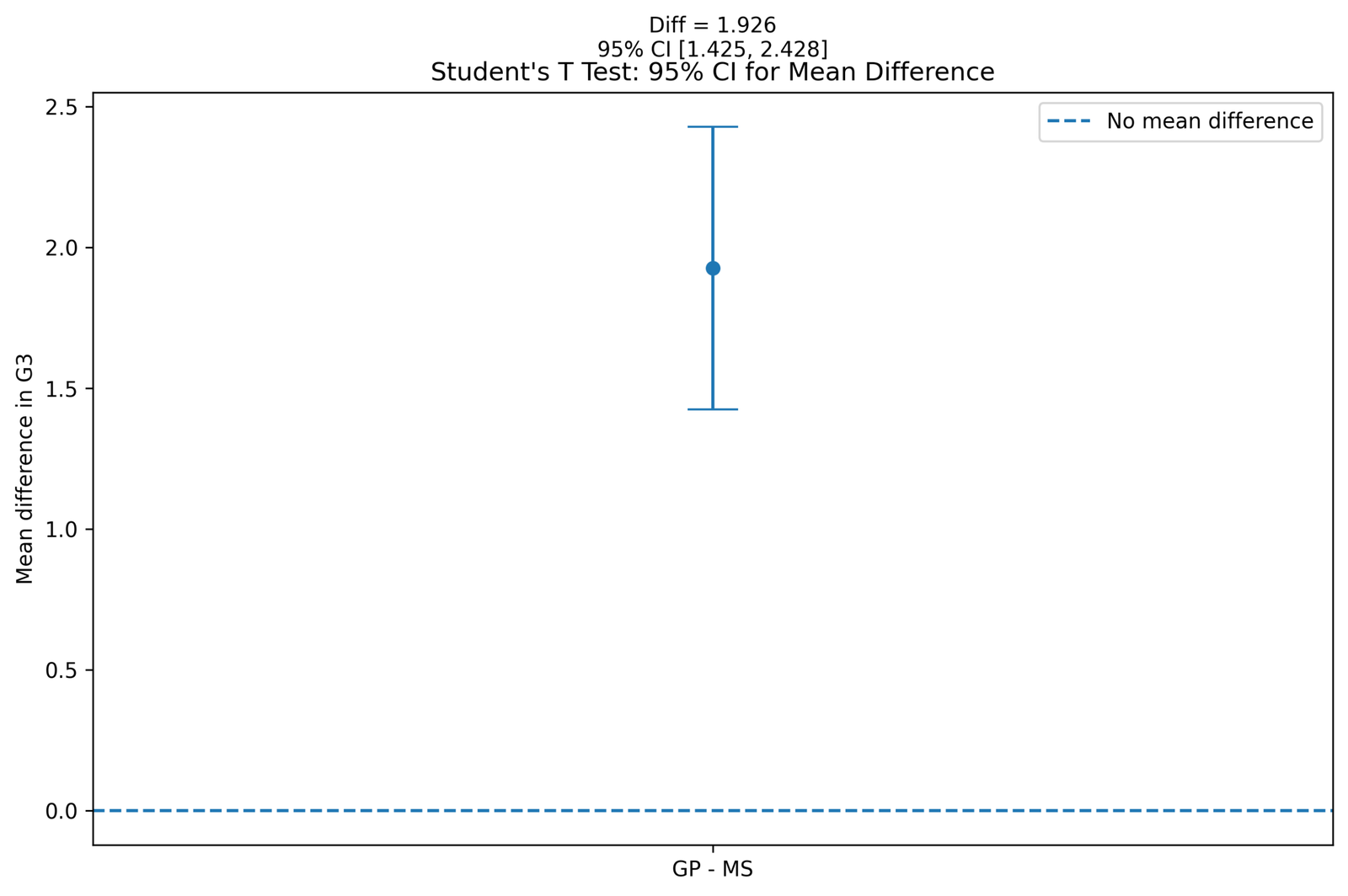
This chart shows the most important inference visually. The mean difference is approximately 1.926, and the 95% confidence interval is approximately 1.425 to 2.428. The entire interval is above zero.
Because zero is not inside the interval, the result supports a significant difference between group means. The positive interval also shows the direction: GP has a higher mean G3 score than MS.
Python Chart 5: Additional Student T Group Mean Comparison
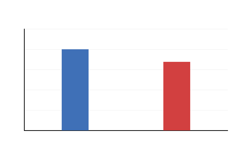
This additional output repeats the group mean comparison. It preserves the supplied chart set and confirms the same visual conclusion: the GP group mean is higher than the MS group mean.
The repeated output is helpful for quality control because the same result appears across multiple exported chart versions.
Python Chart 6: Additional G3 Distribution by Group
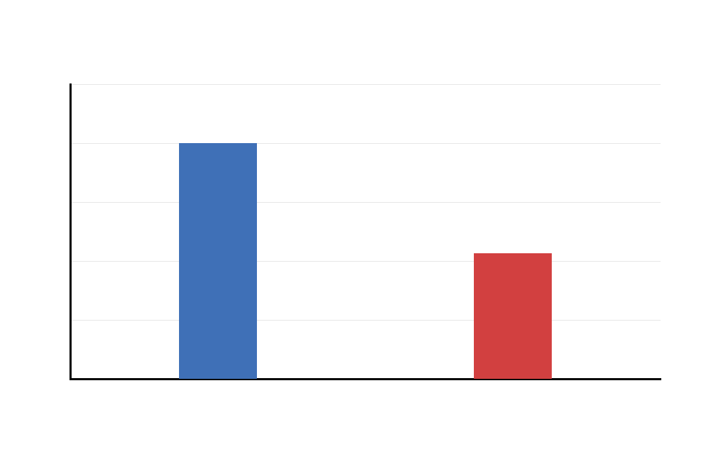
This additional distribution chart confirms the same pattern of group separation and overlap. The GP distribution remains centered higher than the MS distribution.
Distribution charts are important because they show the data pattern behind the mean comparison. They help readers understand whether the result is caused by a visible shift in group scores.
Python Chart 7: Additional Pooled Variance Components
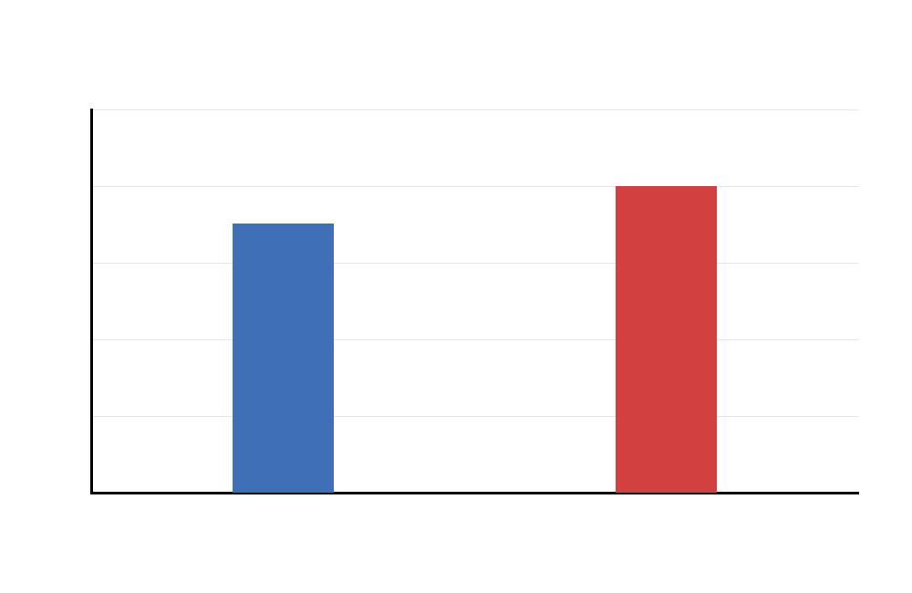
This additional pooled-variance chart repeats the key equal-variance calculation idea. Student’s t-test does not simply compare the two means; it compares the mean difference relative to a pooled estimate of within-group variability.
The chart helps explain why pooled variance is central to the classic Student’s independent t-test.
Python Chart 8: Additional Mean Difference Confidence Interval
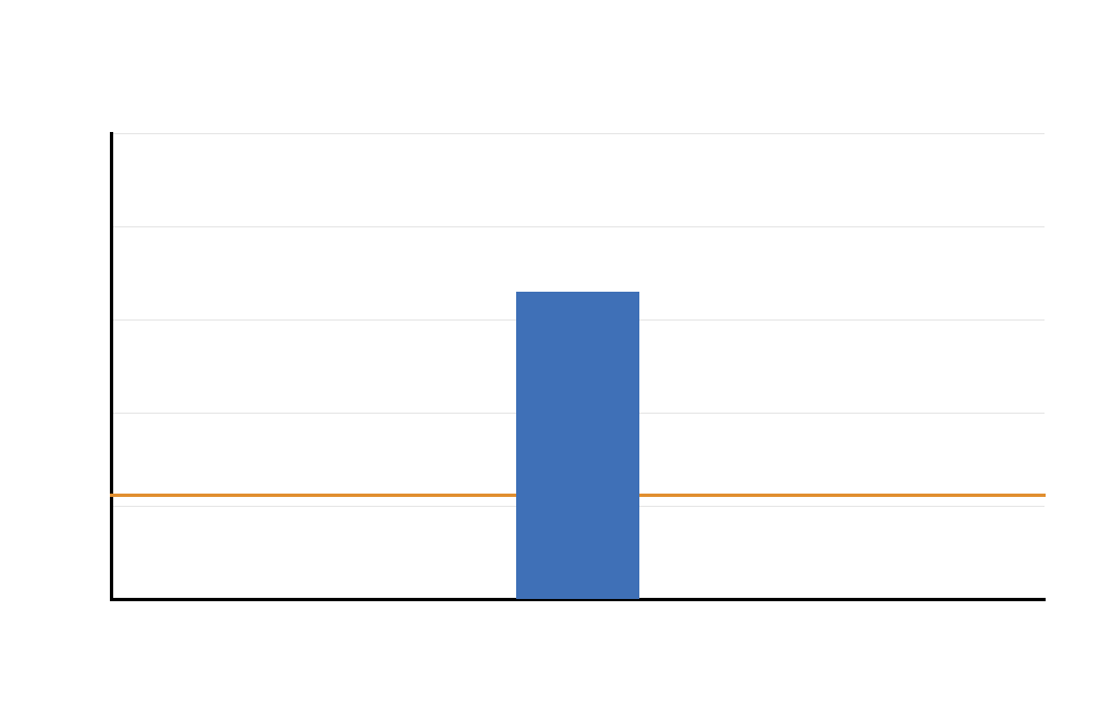
This additional confidence interval output confirms that the mean difference remains positive and statistically significant. The interval does not include zero.
This chart reinforces the final decision: the group difference is reliable, and the GP group has the higher average G3 score.
R Chart-by-Chart Validation
The R charts validate the Python and SPSS conclusions using a separate workflow. The R visual pattern is the same: GP has a higher mean than MS, the group distributions show separation, the pooled variance components support the Student’s t-test calculation, the confidence interval is positive, and the observed t statistic is far from zero. This software-to-software agreement strengthens confidence in the interpretation.
R Chart 1: Student T Group Mean Comparison
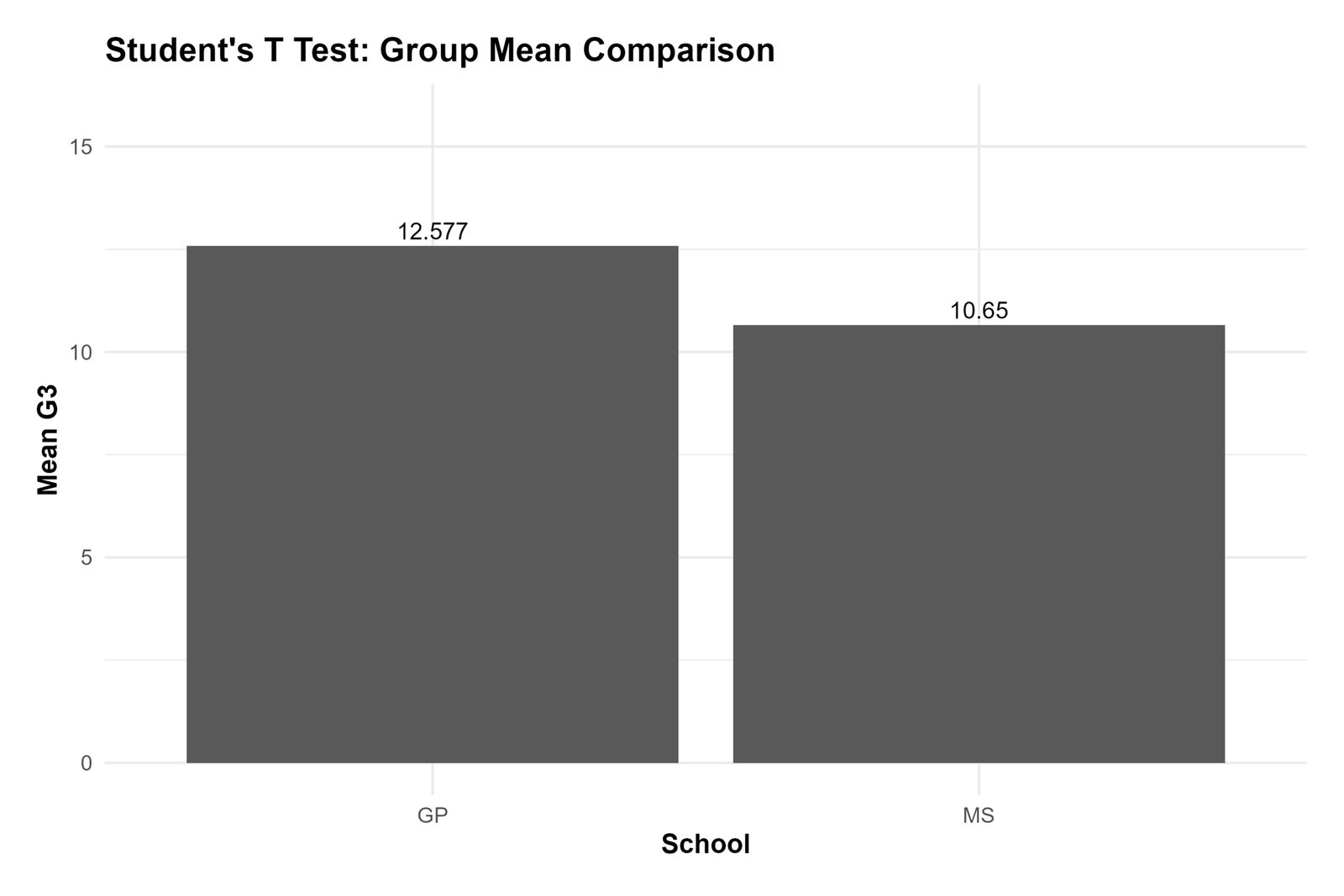
The R group mean comparison confirms the Python result. GP has a higher average G3 score than MS. The difference is visible and aligns with the numerical mean difference of approximately 1.926.
This chart validates that the group mean result is not a software artifact. The same conclusion appears in R and Python.
R Chart 2: G3 Distribution by Group
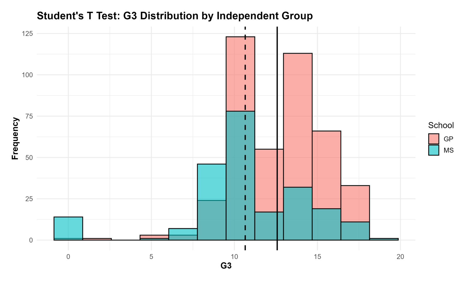
The R distribution chart confirms that the GP distribution is shifted toward higher G3 scores compared with MS. The groups overlap, but the central tendency is clearly higher for GP.
This chart supports the practical interpretation of the Students T Test. The significant result is not just a numerical table result; it is visible in the distribution of scores.
R Chart 3: Pooled Variance Components
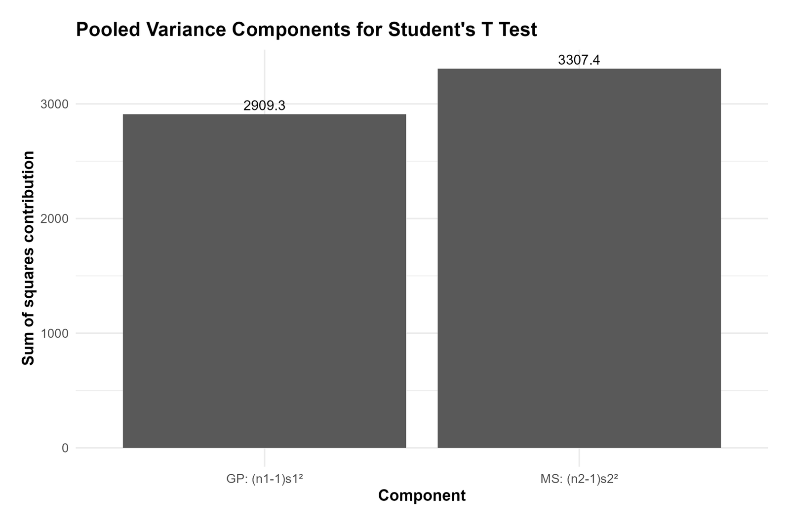
The R pooled-variance chart validates the equal-variance calculation approach. Student’s t-test combines the two group variances into one pooled estimate before calculating the standard error of the mean difference.
This is the key difference between the classic Student’s t-test and Welch’s t test. Student’s t-test assumes a common variance, while Welch’s version does not require equal variances.
R Chart 4: Student T Mean Difference Confidence Interval
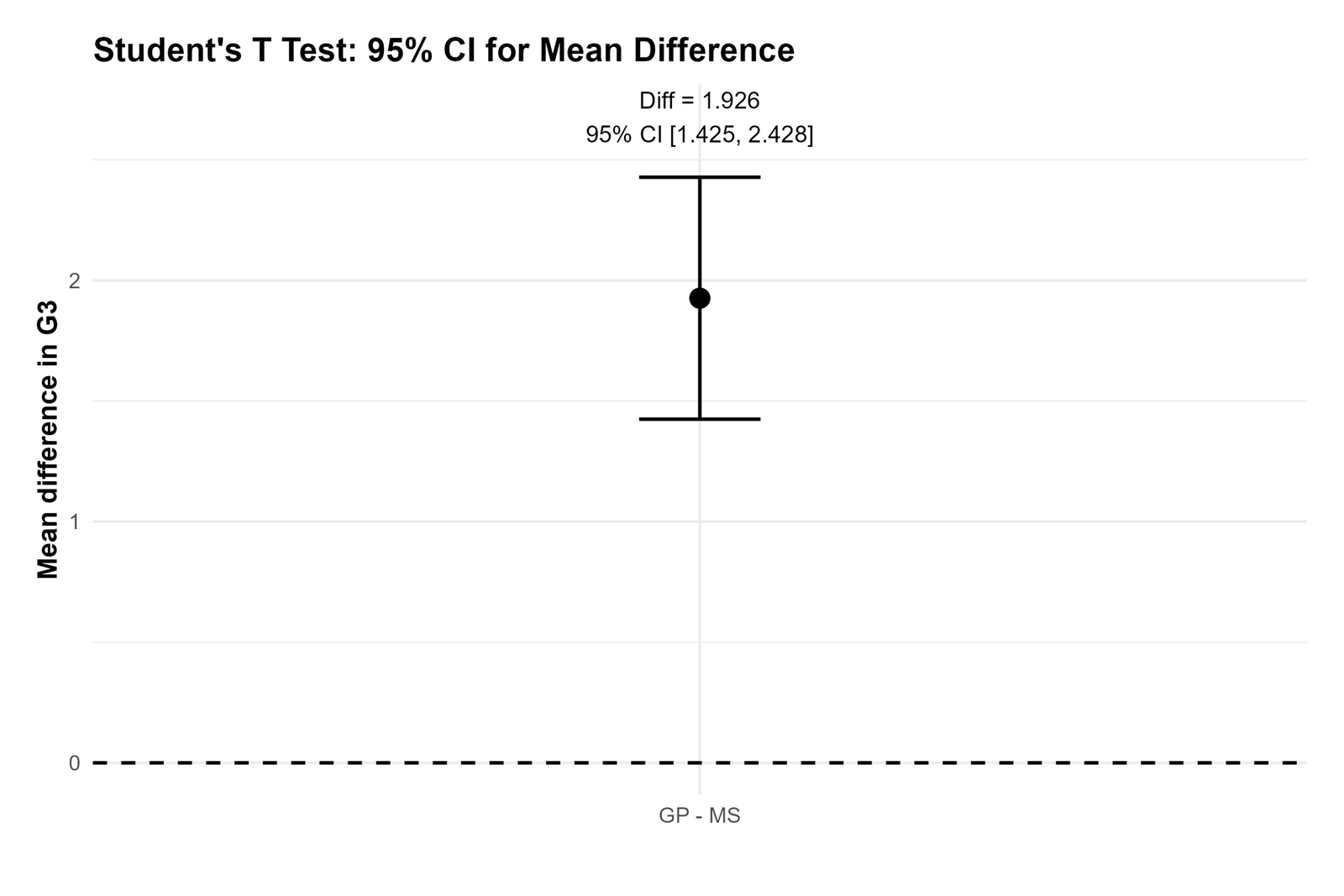
The R confidence interval chart confirms that the mean difference is positive and statistically significant. The entire 95% interval is above zero, so the null hypothesis of equal means is rejected.
This is one of the most useful charts for reporting because it communicates both the size and uncertainty of the difference.
R Chart 5: Student T Distribution with Observed Statistic
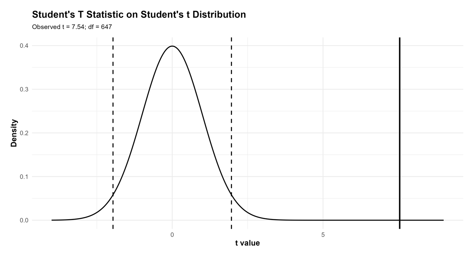
This chart places the observed test statistic on the Student’s t distribution. The observed value is approximately t = 7.54 with df = 647. It is far from the center of the null distribution.
The chart explains why the p value is less than .001. If the null hypothesis of equal means were true, a t statistic this large would be extremely unlikely.
R Chart 6: Group SD Ratio Equal Variance Context
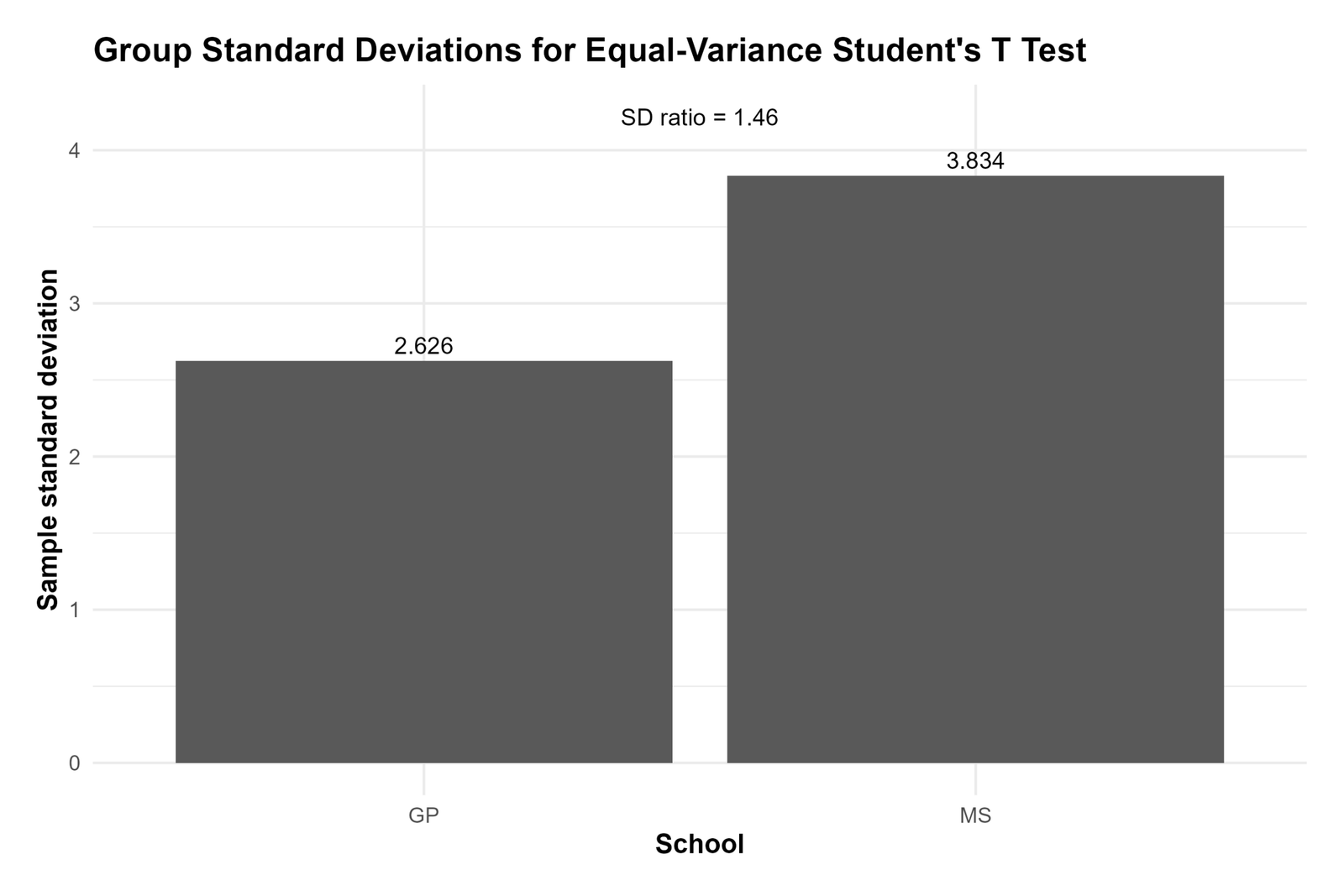
This chart gives important assumption context. The GP standard deviation is approximately 2.626, while the MS standard deviation is approximately 3.834. The MS group has a larger spread.
This does not automatically invalidate the Students T Test, but it does mean that the equal-variance assumption should be checked. In formal reporting, the analyst should mention Levene’s test or compare the Student’s t-test result with Welch’s t test.
R Chart 7: Mean G3 by Study Time and School
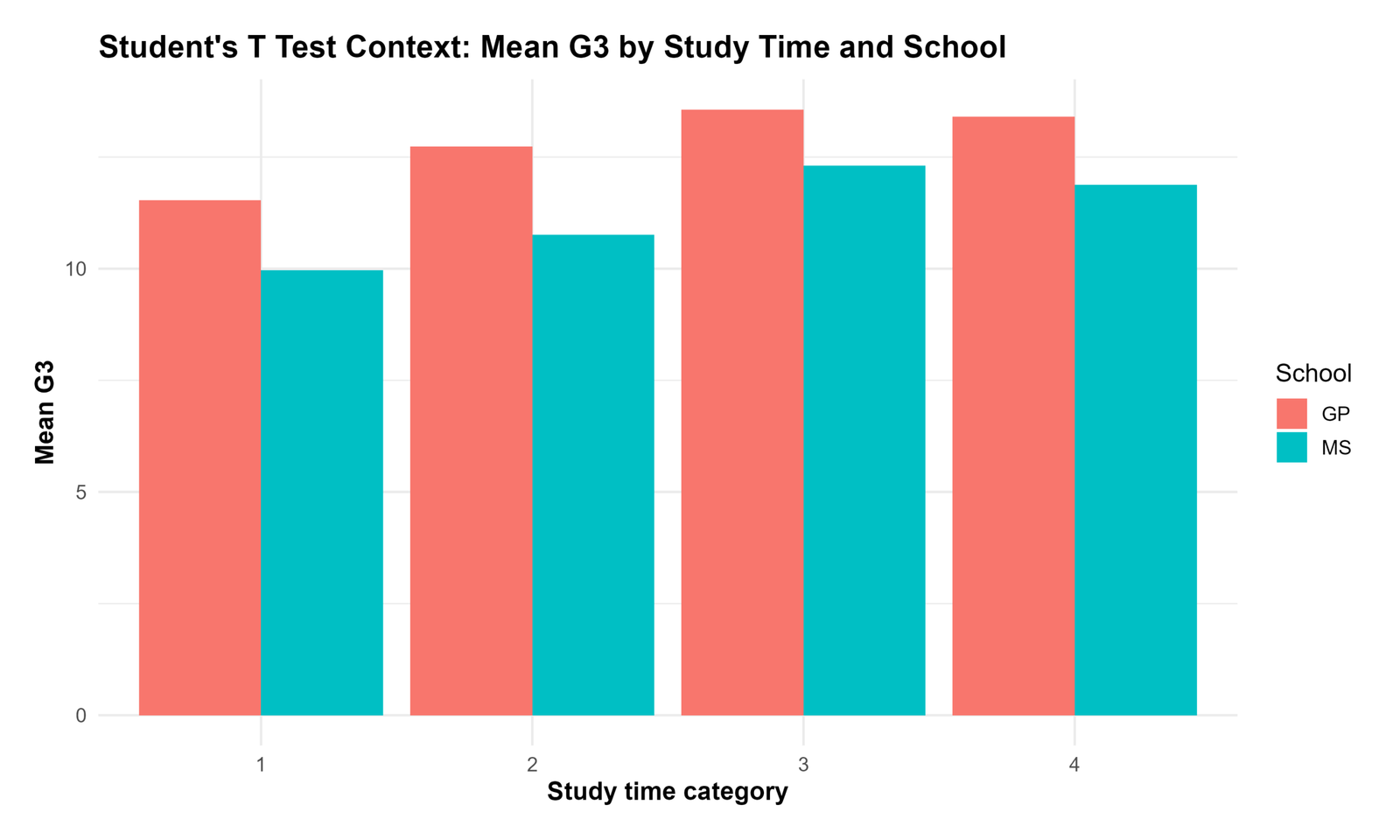
This context chart shows how G3 means vary by study-time level and school group. It helps readers understand whether the overall group difference is consistent across descriptive subgroups.
The chart does not replace the Students T Test because the formal test compares overall school-group means. However, it adds useful interpretation by showing that school differences can be examined alongside study-time patterns.
SPSS, R, Python and Excel Workflows for Students T Test
The same Students T Test workflow can be reproduced in SPSS, R, Python and Excel. SPSS provides the independent samples t test output directly. R can run the equal-variance t test with var.equal = TRUE. Python can calculate the equal-variance t test with scipy.stats.ttest_ind(). Excel can run a two-sample equal variance t test through the Analysis ToolPak or by manual formulas.
SPSS Workflow
| Step | SPSS Menu or Syntax | Purpose |
|---|---|---|
| Open dataset | File > Open > Data | Load the clean dataset. |
| Run test | Analyze > Compare Means > Independent-Samples T Test | Open the two-group mean comparison procedure. |
| Set test variable | Move G3 into Test Variable(s) | Choose final grade as the dependent variable. |
| Set grouping variable | Move school into Grouping Variable | Define GP and MS as the two groups. |
| Check variance assumption | Read Levene’s Test | Decide whether the equal-variance row is appropriate. |
| Interpret output | Read t, df, p and CI | Report the Students T Test result. |
| Export output | File > Export or OUTPUT EXPORT | Save a PDF for reporting and verification. |
R Workflow
| Step | R Action | Purpose |
|---|---|---|
| Read data | read.csv() | Load the dataset. |
| Select variables | G3 and school | Define dependent and grouping variables. |
| Run Student’s t-test | t.test(G3 ~ school, data = df, var.equal = TRUE) | Run the equal-variance two-sample t test. |
| Calculate effect size | Mean difference divided by pooled SD | Estimate Cohen’s d. |
Python Workflow
| Step | Python Action | Purpose |
|---|---|---|
| Read data | pandas.read_csv() | Load the dataset into a DataFrame. |
| Split groups | Filter G3 by school | Create GP and MS samples. |
| Run equal-variance test | stats.ttest_ind(gp, ms, equal_var=True) | Calculate the Student’s t-test statistic and p value. |
| Calculate pooled SD | Manual pooled variance formula | Calculate Cohen’s d and CI. |
| Visualize result | matplotlib | Create mean, distribution, variance and CI charts. |
Excel Workflow
| Excel Task | Formula or Tool | Purpose |
|---|---|---|
| Separate groups | Filter G3 values into GP and MS columns | Prepare the two independent samples. |
| Calculate group means | =AVERAGE(range) | Find each group mean. |
| Calculate group SDs | =STDEV.S(range) | Find each group standard deviation. |
| Run test | Data Analysis ToolPak > t-Test: Two-Sample Assuming Equal Variances | Run the Students T Test in Excel. |
| Calculate p value | Use Excel t-test output or T.DIST.2T() | Interpret statistical significance. |
Code Blocks for Students T Test
SPSS Syntax for Students T Test
* Students T Test / Student's t-test in SPSS.
* Dependent variable: G3.
* Grouping variable: school.
* Groups: GP and MS.

TITLE "Students T Test: G3 by School Group".

T-TEST GROUPS=school('GP' 'MS')
  /VARIABLES=G3
  /MISSING=ANALYSIS
  /CRITERIA=CI(.95).

MEANS TABLES=G3 BY school
  /CELLS MEAN COUNT STDDEV SEMEAN.

OUTPUT EXPORT
  /CONTENTS EXPORT=VISIBLE
  /PDF DOCUMENTFILE="Students-T-Test-SPSS-Output.pdf".
Python Code for Students T Test
import pandas as pd
import numpy as np
from scipy import stats

df = pd.read_csv("dataset.csv")

data = df[["school", "G3", "studytime"]].copy()
data["G3"] = pd.to_numeric(data["G3"], errors="coerce")
data = data.dropna(subset=["school", "G3"])

gp = data.loc[data["school"] == "GP", "G3"]
ms = data.loc[data["school"] == "MS", "G3"]

n1, n2 = len(gp), len(ms)
m1, m2 = gp.mean(), ms.mean()
s1, s2 = gp.std(ddof=1), ms.std(ddof=1)

# Equal-variance Student's t-test
t_stat, p_value = stats.ttest_ind(gp, ms, equal_var=True)

dfree = n1 + n2 - 2

pooled_variance = (((n1 - 1) * s1**2) + ((n2 - 1) * s2**2)) / dfree
pooled_sd = np.sqrt(pooled_variance)

standard_error_difference = pooled_sd * np.sqrt((1 / n1) + (1 / n2))

mean_difference = m1 - m2

critical_t = stats.t.ppf(0.975, dfree)
ci_low = mean_difference - critical_t * standard_error_difference
ci_high = mean_difference + critical_t * standard_error_difference

cohens_d = mean_difference / pooled_sd

print("Students T Test / Student's t-test")
print("GP n =", n1, "mean =", m1, "sd =", s1)
print("MS n =", n2, "mean =", m2, "sd =", s2)
print("Mean difference =", mean_difference)
print("Pooled variance =", pooled_variance)
print("Pooled SD =", pooled_sd)
print("t =", t_stat)
print("df =", dfree)
print("p =", p_value)
print("95% CI =", (ci_low, ci_high))
print("Cohen's d =", cohens_d)
R Code for Students T Test
# Students T Test / Student's t-test in R

df <- read.csv("dataset.csv")

df$G3 <- as.numeric(df$G3)
df$school <- as.factor(df$school)

df_model <- na.omit(df[, c("school", "G3", "studytime")])

# Equal-variance Student's t-test
result <- t.test(G3 ~ school, data = df_model, var.equal = TRUE)
print(result)

gp <- df_model$G3[df_model$school == "GP"]
ms <- df_model$G3[df_model$school == "MS"]

n1 <- length(gp)
n2 <- length(ms)
m1 <- mean(gp)
m2 <- mean(ms)
s1 <- sd(gp)
s2 <- sd(ms)

dfree <- n1 + n2 - 2
pooled_variance <- (((n1 - 1) * s1^2) + ((n2 - 1) * s2^2)) / dfree
pooled_sd <- sqrt(pooled_variance)

mean_difference <- m1 - m2
cohens_d <- mean_difference / pooled_sd

cat("GP n =", n1, "mean =", m1, "sd =", s1, "\n")
cat("MS n =", n2, "mean =", m2, "sd =", s2, "\n")
cat("Mean difference =", mean_difference, "\n")
cat("Pooled variance =", pooled_variance, "\n")
cat("Pooled SD =", pooled_sd, "\n")
cat("Cohen's d =", cohens_d, "\n")
Excel Formulas for Students T Test
Step 1:
Place GP G3 values in one column and MS G3 values in another column.

Step 2:
Calculate group sample sizes:
=COUNT(GP_range)
=COUNT(MS_range)

Step 3:
Calculate group means:
=AVERAGE(GP_range)
=AVERAGE(MS_range)

Step 4:
Calculate group standard deviations:
=STDEV.S(GP_range)
=STDEV.S(MS_range)

Step 5:
Calculate pooled variance:
=(((n1-1)*sd1^2)+((n2-1)*sd2^2))/(n1+n2-2)

Step 6:
Calculate pooled standard deviation:
=SQRT(pooled_variance)

Step 7:
Calculate standard error of mean difference:
=pooled_sd*SQRT((1/n1)+(1/n2))

Step 8:
Calculate t statistic:
=(mean1-mean2)/standard_error_difference

Step 9:
Calculate degrees of freedom:
=n1+n2-2

Step 10:
Calculate two-tailed p value:
=T.DIST.2T(ABS(t_cell),df_cell)

Step 11:
Calculate 95% CI lower:
=(mean1-mean2)-T.INV.2T(0.05,df_cell)*standard_error_difference

Step 12:
Calculate 95% CI upper:
=(mean1-mean2)+T.INV.2T(0.05,df_cell)*standard_error_difference

Step 13:
Calculate Cohen's d:
=(mean1-mean2)/pooled_sd
APA Reporting Wording for Students T Test
The Students T Test should be reported with group means, standard deviations, sample sizes, t statistic, degrees of freedom, p value, confidence interval and effect size. The wording should clearly state the direction of the difference and whether equal variances were assumed.
APA example: An equal-variance Student’s t-test was conducted to compare G3 final grades between GP and MS students. GP students had significantly higher G3 scores (M = 12.58, SD = 2.63, n = 423) than MS students (M = 10.65, SD = 3.83, n = 226), t(647) = 7.54, p < .001. The mean difference was 1.93, 95% CI [1.43, 2.43], with an approximate medium effect size, d = 0.62.
Short reporting version: GP students scored significantly higher on G3 than MS students, t(647) = 7.54, p < .001, 95% CI [1.43, 2.43].
Common Mistakes in Students T Test
| Mistake | Why It Is a Problem | Correct Practice |
|---|---|---|
| Ignoring the equal-variance assumption | Classic Student’s t-test assumes a common variance. | Check Levene’s test or compare with Welch’s t test. |
| Reporting only the p value | The p value does not show size or direction. | Report means, SDs, mean difference, CI and Cohen’s d. |
| Confusing Student’s t-test with all t tests | There are one-sample, paired, independent and Welch versions. | State which version is used. |
| Using paired test for independent groups | GP and MS are independent groups, not repeated measures. | Use independent samples Student’s t-test. |
| Ignoring distribution and outliers | Outliers and spread differences can affect interpretation. | Review histograms, boxplots and group SD ratios. |
| Not reporting effect size | Statistical significance does not show practical size. | Report Cohen’s d or another suitable effect size. |
When to Use Students T Test
Use a Students T Test when you want to compare means using sample-estimated variation and the t distribution. For the independent equal-variance version used in this post, the two groups should be unrelated, the outcome should be numeric, and the equal-variance assumption should be reasonable.
| Use Case | Example | Why Students T Test Fits |
|---|---|---|
| Education | Compare average final grades between two schools. | Two independent groups are compared on a numeric outcome. |
| Business | Compare customer ratings between two service models. | The outcome is numeric and groups are independent. |
| Health research | Compare mean blood pressure between treatment and control groups. | Two independent group means are compared. |
| Manufacturing | Compare average output between two machines. | The test evaluates whether the group means differ. |
Do not use this test when the two observations are paired or repeated measures. For paired observations, use a paired samples t test. If the equal-variance assumption is not reasonable, use Welch’s t test.
Downloads and Resources
Use the following downloadable resources to reproduce the Students T Test workflow in SPSS, Python, R and Excel. Replace the placeholder links with the final hosted file URLs after uploading your scripts and templates to WordPress Media Library.
Download SPSS Syntax
Students T Test syntax with independent samples output export.
Download Python Script
Python workflow with pooled variance, t test, CI, effect size and charts.
Download R Script
R workflow with var.equal = TRUE and validation charts.
Download Excel Template
Excel formulas for pooled variance, t statistic, p value, CI and Cohen’s d.
FAQs About Students T Test
What is a Students T Test?
A Students T Test, commonly written as Student’s t-test, is a statistical test used to compare sample means using the t distribution when population variation is estimated from sample data.
What was tested in this example?
This example compared mean G3 final grade between GP and MS school groups using the equal-variance Student’s t-test approach.
What was the result of the Students T Test?
GP students had a higher mean G3 score than MS students. The result was t(647) = 7.54, p < .001, with a mean difference of 1.926 and a 95% confidence interval of 1.425 to 2.428.
What is pooled variance in Students T Test?
Pooled variance combines the two group variances into one shared estimate of within-group variability. It is used in the equal-variance version of Student’s t-test.
What is the effect size in this example?
The approximate Cohen’s d is 0.62, which is usually interpreted as a medium effect.
When should I use Welch’s t test instead?
Use Welch’s t test when the two groups have noticeably unequal variances or when Levene’s test suggests that the equal-variance assumption is not reasonable.
Can I run Students T Test in Excel?
Yes. Excel can run a two-sample equal variance t test through the Data Analysis ToolPak or by manual formulas for pooled variance, t statistic, degrees of freedom, p value and confidence interval.

