Independent-samples normal-scores test

Van der Waerden Test: 7 Essential Steps, Formula and Worked Example

The Van der Waerden test, also called the normal-scores test, is a powerful nonparametric method for comparing two or more independent groups. It replaces pooled ranks with standard-normal quantiles, then tests whether the groups have the same location distribution. This complete guide explains the formula, assumptions, ties, effect size, post-hoc comparisons, interpretation, and verified workflows in Python, R, SPSS and Excel.

Five independent groups
Normal-score transformation
Omnibus location test
Ties handled by midranks
Python + R + SPSS + Excel

Total sampleN = 649

A-squared33.781995

Degrees of freedom4

Omnibus resultp < .001

Quick answer

Final grades differed significantly across the five maternal-occupation groups.

In the verified Van der Waerden test example, final grade (G3) was compared across five independent maternal-job categories: at home, health, other, services and teacher. After all 649 grades were pooled, tied grades received average ranks, and every pooled rank was converted to a standard-normal score. The omnibus statistic was A² = 33.781995 with 4 degrees of freedom and p = 0.000000825976. At α = .05, the null hypothesis of equal group location distributions was rejected.

The largest positive mean normal scores occurred for the teacher group (0.4430) and the health group (0.3412). The at-home group had the lowest mean normal score (−0.2854). A transformed-score eta-squared of 0.0521 indicates that maternal-job group accounted for about 5.2% of the total variation in the normal scores. This effect-size description should accompany, not replace, the omnibus and post-hoc results.

Correct conclusion: at least one maternal-occupation group tended to produce systematically different final grades. The omnibus result alone does not identify every differing pair, prove a causal effect of maternal occupation, or show that all five distributions differ from one another.

What does the Van der Waerden test measure?

A normal-score comparison of independent population locations.

The Van der Waerden test is a nonparametric omnibus test for comparing the location distributions of two or more independent groups. It starts like the Kruskal–Wallis test by pooling and ranking every observation, but it then transforms each pooled rank into the corresponding quantile of the standard normal distribution. Those transformed values are called normal scores. The Van der Waerden test is most informative when the transformed-score result is interpreted with the original outcome.

The question answered

The practical research question is whether all independent groups tend to generate observations from the same location distribution. Under a clean shift model, this can be described as a test of equal population locations. When group distributions have comparable shape and spread, a significant result indicates that at least one group is shifted upward or downward relative to another.

The method is an omnibus procedure. It evaluates all groups simultaneously and controls the first-stage Type I error more appropriately than running many unadjusted two-sample tests. A significant omnibus result should be followed by planned contrasts or multiplicity-adjusted pairwise comparisons when the research goal requires identifying specific group differences.

Why normal scores are different from ordinary ranks

Ordinary ranks increase in equal one-unit steps. Normal scores do not. Each rank is mapped through the inverse standard-normal cumulative distribution function. Ranks close to the pooled center become scores near zero, while increasingly extreme low and high ranks receive increasingly negative and positive values.

This transformation retains the ordering that makes rank methods robust, while giving the score scale a normal-theory structure. The Van der Waerden test can therefore be highly efficient when the underlying distributions are approximately normal, even though the raw observations are not entered directly into a conventional one-way ANOVA.

Important terminology: “normal-scores test” does not mean a normality test. It does not ask whether the raw data follow a normal distribution. Instead, it deliberately converts pooled ranks to standard-normal quantiles and compares the resulting scores across independent groups. For an actual distributional normality check, see the Shapiro–Wilk test and Q–Q plot normality check.

The null hypothesis is sometimes described as equality of complete population distribution functions and sometimes as equality of group location parameters. These descriptions are compatible only when the shapes and spreads are comparable. If one group differs mainly in spread, skewness or tail weight, the normal-score means can also change. Accordingly, a responsible interpretation examines distribution plots and group summaries before reducing the result to a statement about medians.

When should you use the Van der Waerden test?

Choose it because the design and estimand fit—not merely because a normality p-value is small.

Use the Van der Waerden test for an independent-groups location comparison when the outcome can be meaningfully ordered, a one-factor design contains two or more unrelated groups, and a rank-based method is scientifically appropriate. The method is particularly attractive when near-normal efficiency matters but direct ANOVA assumptions or outlier sensitivity are concerning. The Van der Waerden test belongs in a prespecified analysis plan rather than being selected after comparing p-values.

Independent groups?

Each participant or unit belongs to one group only. Paired, clustered and repeated data need other methods.

Ordered outcome?

The dependent variable must be numeric or at least ordinal with a defensible ordering.

Two or more groups?

The procedure handles a two-sample comparison and extends naturally to k independent samples.

Location question?

The primary question should concern systematic upward or downward differences across groups.

Comparable shapes?

Similar distribution shapes support a direct location-shift interpretation.

Strong use cases

Comparing an ordered clinical response across three independent treatment groups when outliers make raw-score ANOVA fragile.

Comparing student performance across several unrelated school or background categories using a rank-based omnibus method.

Analyzing continuous measurements that are broadly symmetric but not sufficiently well behaved for a classical equal-variance ANOVA.

Seeking a normal-score alternative to Kruskal–Wallis because efficiency near normality is a substantive consideration.

Situations requiring another method

Use the Friedman test for repeated or matched k-group designs rather than treating related observations as independent.

Use the Jonckheere–Terpstra test when groups have a prespecified order and the hypothesis concerns a monotonic trend.

Use a dispersion method such as the Fligner–Killeen test when the research target is variability rather than location.

Use a model that handles clusters, covariates or repeated measures when the design is more complicated than a one-factor independent-samples layout.

Do not select the Van der Waerden test simply because a large-sample Shapiro–Wilk test is significant. With hundreds of observations, normality tests can detect minor departures that have little effect on ANOVA. Conversely, a nonsignificant normality test in a small group does not establish normality. Examine the research question, independence, outliers, group shapes, sample sizes and variance pattern together.

Practical decision rule: use one-way ANOVA when the mean is the intended estimand and its assumptions are defensible; use Welch’s ANOVA when unequal variances are the main parametric concern; use Kruskal–Wallis for a familiar rank-sum approach; and consider the Van der Waerden test when normal scores offer a defensible balance between rank robustness and high efficiency near normality.

Van der Waerden test selection checklist

The Van der Waerden test requires independent observations.

The Van der Waerden test requires an orderable outcome.

The Van der Waerden test pools ranks across all groups.

The Van der Waerden test converts ranks to normal quantiles.

The Van der Waerden test supports two or more groups.

The Van der Waerden test uses k − 1 degrees of freedom.

The Van der Waerden test needs explicit tie handling.

The Van der Waerden test is followed by adjusted comparisons after rejection.

The Van der Waerden test does not establish causality.

The Van der Waerden test should be reported with an effect-size description.

Van der Waerden test assumptions: seven checks

Nonparametric methods replace some assumptions; they do not eliminate design requirements.

The Van der Waerden test assumptions should be evaluated before interpreting the chi-square p-value as a pure location result. The most important conditions concern independence, measurement ordering, sampling design, meaningful group labels, and comparable distributional shape. The Van der Waerden test remains a design-based procedure, so independence cannot be repaired by transformation.

Independent observations

No individual, classroom, patient, device or experimental unit should contribute multiple observations that are analyzed as though unrelated. Dependence usually makes the nominal reference distribution too optimistic.

Independent groups

Group membership must be mutually exclusive for the one-factor design. A person cannot simultaneously belong to multiple maternal-job categories in the same analysis row.

Ordered response

The dependent variable must support ranking. Numeric measurements work naturally. Ordinal scales require enough meaningful levels to justify treating greater scores as greater outcomes.

Representative design

Generalization requires random sampling, random assignment or another design that supports the intended population inference. A small p-value does not repair selection bias.

Comparable shape and spread

When group distributions have similar shape and dispersion, differences in mean normal scores are most clearly interpreted as location shifts.

Transparent tie handling

Tied observations should receive pooled average ranks before the inverse-normal transformation. With discrete grades, ties are a major feature rather than a minor computational detail.

Seventh check: enough information in the outcome

The Van der Waerden test can be computed for an ordinal outcome, but power and interpretation depend on the number and distribution of distinct values. The worked dataset contains 649 grades but only 17 observed grade values. Grade 11 appears 104 times, grade 10 appears 97 times and grade 13 appears 82 times. These ties reduce the number of distinct score levels, although the midrank transformation remains fully auditable.

An outcome with only two categories should usually be analyzed as binary rather than forced into a rank test. An outcome with three or four heavily imbalanced categories may also be better addressed with ordinal or multinomial modeling. The existence of a numerical code does not automatically make an outcome suitable for a normal-scores analysis.

Shape differences change the meaning. If one group is strongly skewed, another is symmetric and a third contains a heavy upper tail, rejection of the omnibus null cannot be summarized safely as “the medians differ.” The test indicates systematic differences in the ranked-and-transformed observations. Distribution plots and descriptive summaries must determine whether a simple location-shift narrative is reasonable.

Equal sample sizes are not required. The current groups range from 48 observations in health to 258 in other. Unequal sample sizes are valid, but they affect precision and the contribution of each group to the omnibus statistic. A small group with a large mean score can be scientifically important while contributing less weighted evidence than a much larger group.

Van der Waerden test hypotheses and data dictionary

Define the population statement and the exact variables before calculating ranks.

The Van der Waerden test evaluates an omnibus null across independent groups. In a location-shift interpretation, the null states that all population locations are equal. In the more general distributional wording, all groups have the same population distribution function. The Van der Waerden test links the formal null to the observed group coding used in the analysis.

Formal hypotheses

H₀: F₁(x) = F₂(x) = ··· = F_k(x)

All k population distribution functions are equal. Under comparable shape and spread, this is commonly interpreted as equality of population locations.

H_A: F_i(x) ≠ F_j(x) for at least one pair i ≠ j

At least one population tends to yield systematically different observations. The omnibus alternative does not state which pair differs or in which direction.

For the current five-group example, rejecting H₀ means that the final-grade distributions are not all equivalent across the maternal-job categories. It does not mean that every pair is significant.

Variables used in the worked analysis

OutcomeG3, the numeric final grade.

Grouping variableMjob, maternal occupation.

Categoriesat_home, health, other, services and teacher.

Complete rows649 observations.

Observed outcome range0 to 19.

Overall centerMean = 11.9060; median = 12.

What is being compared after transformation?

Each grade receives a pooled midrank. The pooled midrank is divided by N + 1 and passed through the inverse standard-normal cumulative distribution function. The test then compares the weighted group means of those normal scores.

A group with a negative mean normal score tends to occupy lower pooled ranks. A group with a positive mean normal score tends to occupy higher pooled ranks. Because the overall score distribution is centered close to zero, the group means provide an intuitive direction summary.

What is not established by the hypotheses?

The hypotheses do not establish causality, equal variances, normal raw data, or a particular numerical difference in means. Maternal occupation may be associated with many socioeconomic, educational and contextual variables. The test evaluates the observed group distributions; it does not isolate a causal mechanism.

The test also does not provide a raw-grade confidence interval automatically. Pairwise normal-score comparisons locate differences on the transformed scale, while raw medians and means help readers understand their practical direction.

Applied hypothesis decision

The observed statistic was A² = 33.7819947516. Under H₀, the large-sample reference distribution is chi-square with k − 1 = 4 degrees of freedom. The right-tail probability was p = 8.259763 × 10⁻⁷. Because this value is far below α = .05, the equal-distribution null was rejected.

The result is statistically decisive, but the transformed-score effect size is not enormous: η²_NS = A²/(N − 1) = 0.0521. This means that group membership accounts for approximately 5.2% of total variation in the normal scores. Statistical significance and practical magnitude should therefore be reported separately.

Van der Waerden test formula and normal-score calculation

Every step can be reproduced from pooled midranks, inverse-normal scores and weighted group means.

The Van der Waerden test formula converts the pooled rank of each observation to a normal score. The omnibus statistic measures how far the group mean normal scores are spread from zero relative to the total variance of all transformed scores. The Van der Waerden test calculation is fully reproducible because every score can be traced to a pooled midrank.

Step 1: pool all observations and assign midranks

Let N be the total number of observations and R_i be the pooled rank of observation i. Rankings are ascending, so the smallest observation receives the lowest rank. When several observations share the same value, each receives the average of the ranks that the tied block would occupy.

R_i = pooled ascending midrank of X_i

In the current dataset, all students with G3 = 11 share the same pooled midrank of 249.5 because the 104 tied grade-11 observations span a block of pooled rank positions.

Step 2: convert every rank to a normal score

z_i = Φ⁻¹[R_i/(N + 1)]

Φ⁻¹ is the inverse cumulative distribution function of a standard normal variable. Dividing by N + 1 keeps the probability strictly between zero and one, preventing infinite scores at the endpoints.

For example, with N = 649, a pooled midrank of 249.5 gives a plotting position of 249.5/650 = 0.383846. Its inverse-normal score is approximately −0.295395. A pooled midrank of 618 gives a plotting position of 0.950769 and a normal score of approximately 1.652358.

Step 3: calculate each group mean normal score

z̄_j = (1/n_j) ∑_i∈j z_i

n_j is the sample size in group j. Positive values indicate generally higher pooled positions; negative values indicate generally lower pooled positions.

Step 4: calculate the overall normal-score variance

s_z² = [∑_i=1^N z_i²]/(N − 1)

The pooled normal scores are centered extremely close to zero by construction. The verified score variance for this dataset is 0.9511039611, slightly below one because the outcome contains many ties and therefore fewer distinct transformed values.

Step 5: calculate the omnibus statistic

A² = [∑_j=1^k n_jz̄_j²]/s_z²

Large weighted deviations of group mean scores from zero produce a large A² statistic. Under H₀, A² is referred approximately to a chi-square distribution with k − 1 degrees of freedom.

Step 6: obtain the p-value

p = P[χ²_k−1 ≥ A²]

For A² = 33.781995 and df = 4, the right-tail probability is 0.000000825976. The observed between-group separation on the normal-score scale is therefore highly unlikely under equal group distributions.

Step 7: report a transformed-score effect size

η²_NS = A²/(N − 1) = 0.052133

This ratio equals the between-group sum of squares divided by the total sum of squares on the normal-score scale. It is a descriptive proportion of transformed-score variation, not a raw-grade variance-explained measure.

Why ties matter: if grade 11 occurs 104 times, assigning arbitrary sequential ranks would give identical grades different normal scores and make the result depend on row order. Midranks ensure that every identical observed value receives the same score. The workbook, Python and R calculations all use pooled average ranks.

Van der Waerden test example: final grades by maternal occupation

A complete analysis using 649 observations and five independent groups.

This Van der Waerden test example compares final grades across maternal-job categories. The analysis reports raw descriptives, transformed-score means, the omnibus calculation, effect size and adjusted pairwise comparisons instead of presenting an isolated p-value. The Van der Waerden test example demonstrates why raw summaries and transformed summaries should be reported together.

Research scenario

The outcome G3 records each student’s final grade. Mjob identifies the maternal occupation category. The substantive question is whether the distribution of final grades is equivalent across at-home, health, other, services and teacher groups.

The design is observational. The groups are treated as independent because each row represents one student and each student has one maternal-job classification. Maternal occupation is not randomly assigned, so the results should be interpreted as an association rather than a causal effect.

Overall data profile

The complete analysis contains 649 students. Across all groups, the final-grade mean is 11.9060, the standard deviation is 3.2307, the median is 12, and the interquartile range runs from 10 to 14. The observed range is 0 to 19.

The outcome is discrete and highly tied. Only 17 distinct grade values occur. This makes the exact rank-to-score lineage especially important because every tied grade block must share a pooled midrank.

Mjob group	n	Mean G3	SD	Median	IQR	Min–max	Mean normal score
at_home	135	11.0444	3.1383	11	3.00	0–18	−0.2854
health	48	13.0625	2.9565	13	4.25	8–18	0.3412
other	258	11.6705	3.3072	12	4.00	0–18	−0.0630
services	136	12.1471	2.9175	12	4.00	0–19	0.0537
teacher	72	13.1389	3.3073	13	4.00	0–19	0.4430

Lowest score mean−0.2854at_home

Highest score mean0.4430teacher

Omnibus A²33.7820df = 4

Effect size0.0521normal-score η²

The raw descriptives and transformed means tell a consistent story. Teacher and health have raw means just above 13 and medians of 13; both groups also have positive mean normal scores. At_home has the lowest raw mean, the lowest median and the most negative mean normal score. Other and services sit between these extremes.

However, descriptive ordering is not equivalent to inferential significance. Health has only 48 observations, while other has 258. The pairwise standard error therefore depends on both group sizes as well as the residual variation in the normal scores. Adjusted post-hoc results are needed before stating which pairs remain distinguishable after multiplicity control.

Worked calculation: the weighted between-group normal-score term is A² × s² = 33.7819948 × 0.9511040 ≈ 32.127. Dividing that weighted separation by the pooled normal-score variance returns A² = 33.781995. Referring this value to χ²(4) produces p = 8.2598 × 10⁻⁷.

Van der Waerden test results and Holm-adjusted pairwise findings

The significant omnibus result is followed by comparisons on the same normal-score scale.

The verified Van der Waerden test results reject equal distributions across the five maternal-job groups. Pairwise normal-score comparisons identify six significant differences after Holm family-wise adjustment and four comparisons that do not remain significant. The Van der Waerden test result becomes actionable only after a defensible multiplicity-adjusted follow-up.

Primary inference

A² = 33.782

With df = 4, the exact reported probability is 8.2598 × 10⁻⁷. The omnibus null is rejected at .05, .01 and .001.

At least one group differs

Calculation audit

Number of observations649

Number of groups5

Score variance0.9511039611

A² statistic33.7819947516

p-value0.000000825976

Holm-adjusted pairwise comparisons

Pair	Mean-score difference	t-like statistic	Unadjusted p	Holm-adjusted p	Decision
at_home − health	−0.6266	−3.9149	0.000100	0.000801	Significant
at_home − other	−0.2223	−2.1976	0.028331	0.113325	Not significant
at_home − services	−0.3390	−2.9300	0.003510	0.024571	Significant
at_home − teacher	−0.7284	−5.2405	0.000000217	0.000002173	Significant
health − other	0.4043	2.7002	0.007111	0.035556	Significant
health − services	0.2876	1.7984	0.072584	0.217752	Not significant
health − teacher	−0.1018	−0.5735	0.566497	0.566497	Not significant
other − services	−0.1167	−1.1563	0.247991	0.495983	Not significant
other − teacher	−0.5060	−3.9864	0.0000748	0.000673	Significant
services − teacher	−0.3893	−2.8048	0.005186	0.031115	Significant

The post-hoc pattern places teacher and health toward the upper end of the transformed distribution and at_home toward the lower end. Teacher differs from at_home, other and services, but not from health. Health differs from at_home and other, but not from services or teacher. The at_home and other comparison has an unadjusted p-value below .05 but does not survive Holm adjustment, illustrating why raw pairwise p-values should not be interpreted in isolation.

Multiplicity matters: ten pairwise hypotheses are examined. Holm’s procedure orders the unadjusted p-values and applies progressively less stringent thresholds while controlling the family-wise error rate. It is uniformly at least as powerful as simple Bonferroni adjustment and should be stated explicitly in the report.

These pairwise comparisons are computed on the normal-score scale using the residual scaling associated with the omnibus test. They are not ordinary raw-grade t tests. The signs help explain direction, while the adjusted p-values determine which comparisons remain statistically reliable after accounting for the family of ten tests.

Van der Waerden test in Python: verified calculation and charts

A transparent implementation using pooled ranks, inverse-normal scores and a chi-square tail probability.

The Van der Waerden test in Python can be reproduced directly with SciPy building blocks. The workflow below avoids a black-box result: it stores every pooled midrank and normal score, summarizes each group, computes the omnibus statistic and reports the transformed-score effect size. The Van der Waerden test in Python is especially transparent when row-level ranks and scores are retained.

Python

import numpy as np

import pandas as pd

from scipy.stats import rankdata, norm, chi2
df = pd.read_csv("dataset.csv")

work = df.loc[:, ["G3", "Mjob"]].dropna().copy()
# 1. Pooled midranks, including averaged ranks for ties

N = len(work)

work["rank"] = rankdata(work["G3"], method="average")
# 2. Van der Waerden normal scores

work["normal_score"] = norm.ppf(work["rank"] / (N + 1))
# 3. Group counts and group mean normal scores

summary = (

work.groupby("Mjob", observed=True)["normal_score"]

.agg(n="size", mean_score="mean")

)
# 4. Normal-score variance and omnibus statistic

s2 = (work["normal_score"] ** 2).sum() / (N - 1)

A2 = ((summary["n"] * summary["mean_score"] ** 2).sum()) / s2

df_chi = len(summary) - 1

p_value = chi2.sf(A2, df_chi)

eta2_ns = A2 / (N - 1)

print(summary) print(f"A^2 = {A2:.12f}") print(f"df = {df_chi}") print(f"p = {p_value:.12g}") print(f"normal-score variance = {s2:.12f}") print(f"eta-squared on normal scores = {eta2_ns:.6f}")

Expected verified output: A² = 33.781994751624, df = 4, p = 8.25976322260e−07, normal-score variance = 0.951103961068 and η²_NS = 0.052133.

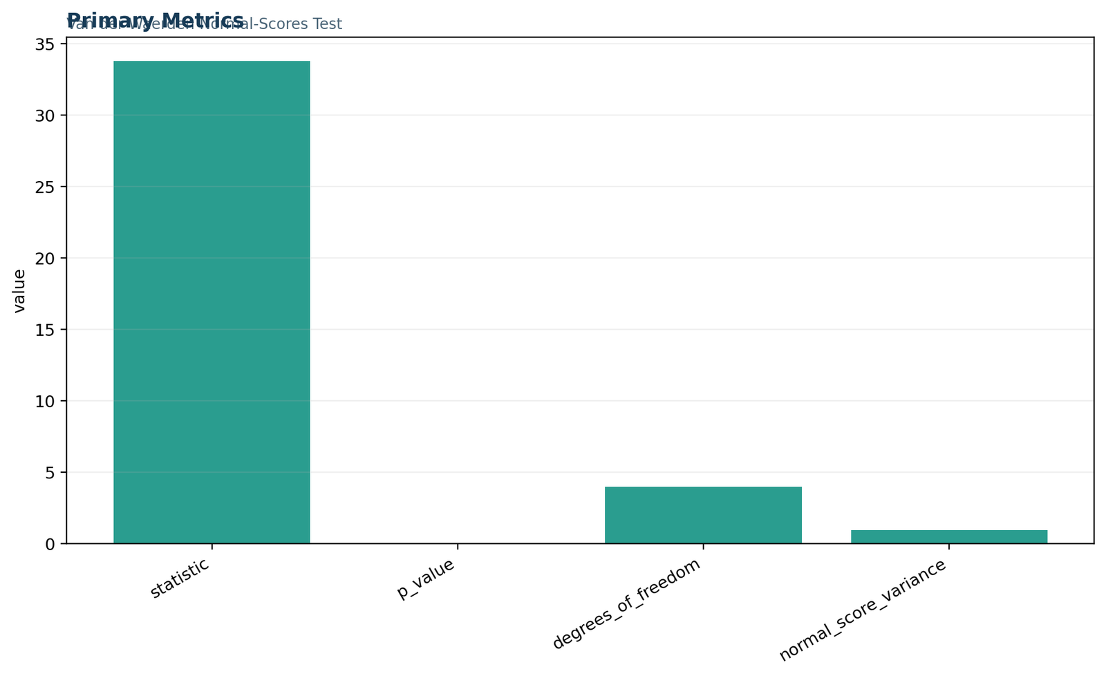
Python primary metrics for the Van der Waerden test — Python chart 1: primary metrics
The statistic dominates the chart at 33.782, while the p-value is visually near zero on the same axis. Degrees of freedom equal four and the normal-score variance is 0.9511. Because these quantities use different units, the chart is best treated as a compact verification panel rather than a magnitude comparison among metrics.

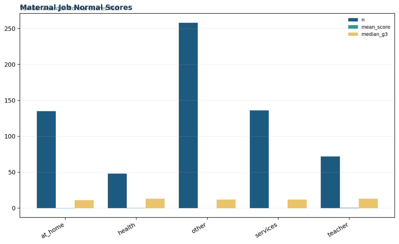
Python maternal job group sizes and mean normal scores — Python chart 2: maternal-job normal scores
The bars show major group-size imbalance—other has 258 students, whereas health has 48—alongside transformed location summaries. Teacher has the highest mean score (0.4430), followed by health (0.3412). At_home is the only group with a clearly negative mean score (−0.2854), while other (−0.0630) and services (0.0537) are close to the pooled center.

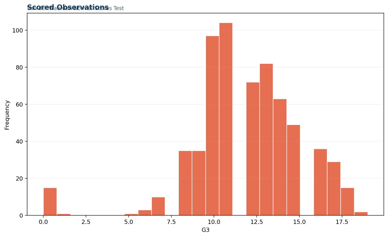
Python histogram of G3 scored observations used in the Van der Waerden test — Python chart 3: scored observations
The grade histogram exposes the large tied blocks that drive the midrank calculation. Grade 11 occurs 104 times, grade 10 occurs 97 times and grade 13 occurs 82 times. Every observation in a tied block receives the same pooled midrank and therefore the same normal score; arbitrary row-order ranks would be invalid.

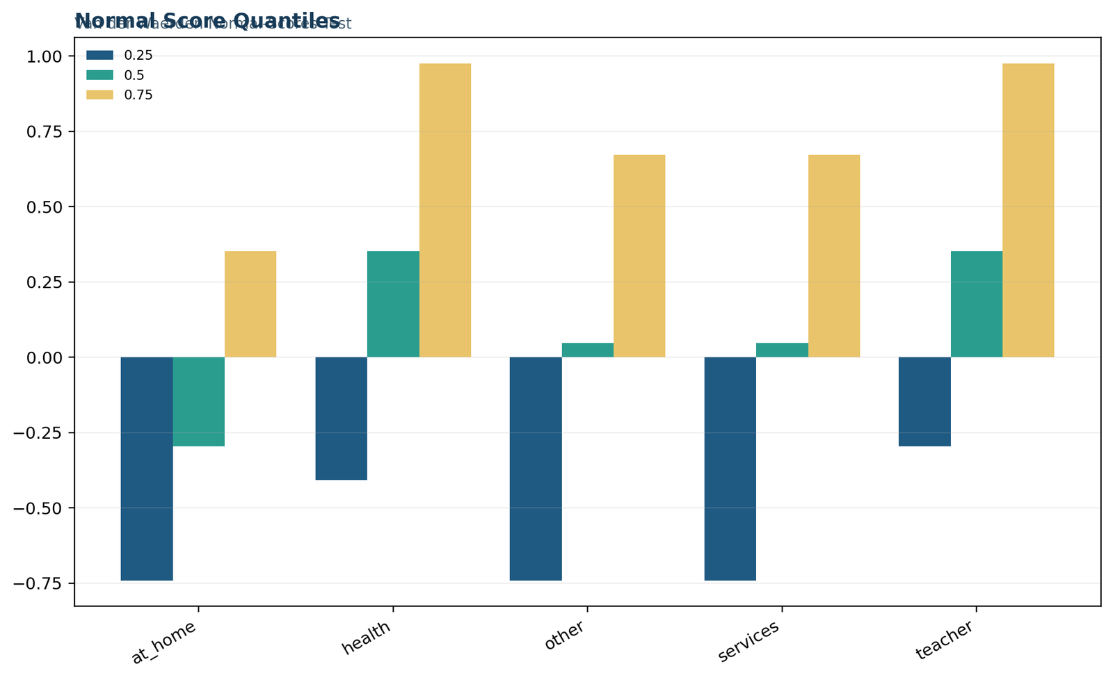
Python quartiles of Van der Waerden normal scores by maternal occupation — Python chart 4: normal-score quantiles
The transformed quartiles reinforce the group ordering. At_home has normal-score quartiles of approximately −0.741, −0.295 and 0.352. Teacher and health have medians near 0.352 and upper quartiles near 0.976. Other and services share quartiles near −0.741, 0.048 and 0.672, although their group means differ slightly.

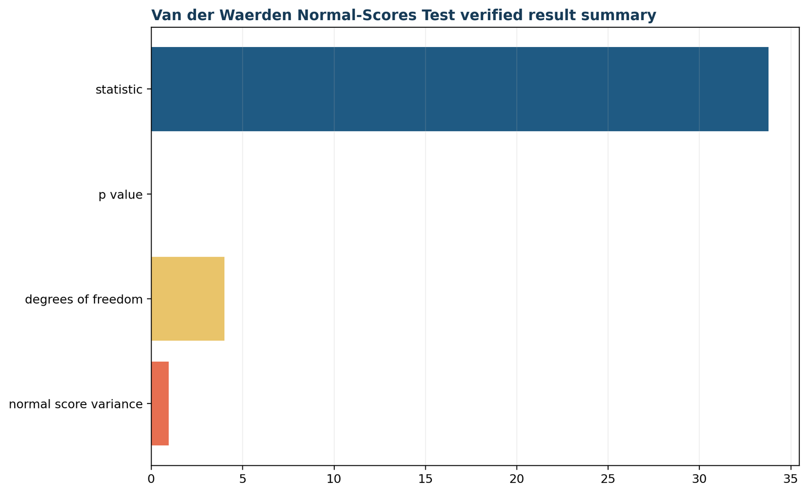
Python verified Van der Waerden result summary — Python chart 5: verified result summary
The final audit chart repeats A² = 33.782, df = 4 and normal-score variance = 0.9511. Its p-value bar is effectively invisible because 8.26 × 10⁻⁷ is tiny relative to the other metrics. The written caption is therefore essential for accessibility and exact reporting.

Python quality check: do not calculate ranks separately inside each group. The ranks must be pooled across all five groups before transformation. Group-specific ranks would erase the between-group location information and produce a fundamentally different analysis.

Van der Waerden test in R: package output and manual verification

Use a dedicated function, then reproduce its core calculations for a complete audit trail.

The Van der Waerden test in R is available through packages such as DescTools and PMCMRplus. The code below runs the formula interface and then independently reconstructs the normal scores, group means, A² statistic, chi-square p-value and effect size. The Van der Waerden test in R should be checked against a manual implementation when ties are prominent.

# install.packages("DescTools")  # run once if needed

library(DescTools)
dat <- read.csv("dataset.csv")

dat <- dat[complete.cases(dat[, c("G3", "Mjob")]), c("G3", "Mjob")]

dat$Mjob <- factor(dat$Mjob)
# Package result

VanWaerdenTest(G3 ~ Mjob, data = dat)
# Transparent manual reproduction

N <- nrow(dat)

dat$pooled_midrank <- rank(dat$G3, ties.method = "average")

dat$normal_score <- qnorm(dat$pooled_midrank / (N + 1))
group_n <- table(dat$Mjob)

group_mean_score <- tapply(dat$normal_score, dat$Mjob, mean)

score_variance <- sum(dat$normal_score^2) / (N - 1)
A2 <- sum(as.numeric(group_n) * group_mean_score^2) / score_variance

df_chi <- nlevels(dat$Mjob) - 1

p_value <- pchisq(A2, df = df_chi, lower.tail = FALSE)

eta2_ns <- A2 / (N - 1)

data.frame( group = names(group_n), n = as.numeric(group_n), mean_normal_score = as.numeric(group_mean_score) ) c(A2 = A2, df = df_chi, p_value = p_value, normal_score_variance = score_variance, eta2_normal_scores = eta2_ns)

The direct calculation is valuable because package implementations may differ in details such as naming, tie notes, printed precision or post-hoc support. A report should verify the score convention rather than assume that every function with a similar name uses an identical formula.

R primary metrics for the Van der Waerden normal scores test — R chart 1: primary metrics
The R pipeline reproduces the same four primary quantities as Python and the workbook. Agreement to numerical precision is the central validation: A² = 33.781995, df = 4, p = 8.2598 × 10⁻⁷ and s² = 0.951104.

R maternal occupation group sizes and mean normal scores — R chart 2: group normal-score profile
The normal-score means align with the raw-grade ordering without being identical to raw means. Teacher and health occupy the highest pooled positions, at_home the lowest, and services and other cluster closer to zero. The n bars remind readers that precision differs substantially by group.

R frequency chart of final grades transformed for the Van der Waerden test — R chart 3: frequency structure and ties
The same tied-grade structure appears in the R output. This chart is methodologically important because the test is not using 649 unique ranks. It is using 17 distinct grade values, each mapped to an averaged pooled rank and a shared normal score.

R normal score quartiles by maternal occupation — R chart 4: transformed quartile comparison
Teacher and health have the highest median and upper-quartile normal scores. At_home is shifted downward across the transformed quartiles. Similar quartiles for other and services explain their nonsignificant adjusted pairwise comparison despite a small difference in group mean scores.

R verified result summary for Van der Waerden test — R chart 5: final numerical reconciliation
The result summary closes the audit loop among R, Python and Excel. A publication-ready workflow should not accept a result until the group counts, score means, statistic, degrees of freedom, p-value and score variance reconcile across independent implementations.

R interpretation tip: package output may describe the null as equal location parameters or equal distributions. Use the stronger location wording only when group shapes and spreads are sufficiently comparable. Otherwise report that the distributions of the ranked-and-transformed outcome differ.

Van der Waerden test in SPSS: exact workflow and limitations

SPSS can create pooled normal scores and diagnostics; the supplied report and workbook verify the custom omnibus calculation.

A Van der Waerden test in SPSS is not reliably obtained by selecting a different nonparametric menu command and renaming the output. The correct workflow must pool ranks, transform them with the inverse normal function and calculate the Van der Waerden A² statistic or call verified Python/R code through SPSS integration. The Van der Waerden test in SPSS must preserve the exact score convention rather than substitute another menu test.

What SPSS can do directly

SPSS can filter complete rows, create pooled average ranks, compute inverse-normal scores, produce group descriptives and graph the transformed distributions. These steps are valuable because they verify data coding and show whether the group-ordering narrative is consistent with the exact workbook result.

A one-way ANOVA on the transformed scores can be used as a diagnostic view, but its printed F statistic should not automatically be reported as the chi-square Van der Waerden A² statistic. The supplied SPSS PDF and Excel workbook preserve the exact method identity.

What must not be substituted

Kruskal–Wallis, median test, one-way ANOVA on raw grades and a generic normal-score transformation are related but not interchangeable. They use different statistics and can produce different p-values. A valid report must label the procedure that was actually calculated.

Similarly, “normal scores” in a rank dialog may use alternative plotting-position formulas. The verified formula in this analysis is Φ⁻¹[R/(N + 1)] with pooled average ranks for ties.

SPSS syntax

* Keep the analysis variables and remove incomplete rows.

DATASET NAME vdw.

SELECT IF NOT MISSING(G3) AND NOT MISSING(Mjob).

EXECUTE.
* Add the total N to every row.

AGGREGATE

OUTFILE=* MODE=ADDVARIABLES

/BREAK=

/N_TOTAL=N.
* Pooled ascending midranks with mean ranks for ties.

RANK VARIABLES=G3 (A)

/RANK INTO R_G3

/TIES=MEAN.
* Convert each pooled rank to a standard-normal quantile.

COMPUTE NS_G3=IDF.NORMAL(R_G3/(N_TOTAL+1),0,1).

COMPUTE NS2=NS_G3**2.

EXECUTE.
* Descriptive verification on the transformed outcome.

MEANS TABLES=NS_G3 G3 BY Mjob

/CELLS=COUNT MEAN MEDIAN STDDEV MIN MAX.

* For the exact A-squared calculation, use the supplied workbook * or run the matching Python/R code through SPSS integration. * A one-way analysis of NS_G3 is useful as a diagnostic but should * not be relabeled as the chi-square Van der Waerden statistic.

Verified SPSS reporting values: N = 649, five groups, A² = 33.781995, df = 4 and p = 8.2598 × 10⁻⁷. Use the downloadable SPSS output for the software-specific audit and the workbook for the exact formula trail.

Before running the syntax, verify that Mjob is a categorical grouping variable and G3 is numeric. Inspect value labels carefully. A hidden trailing space, inconsistent capitalization or accidental numeric recoding can split one conceptual category into multiple groups and change both k and the degrees of freedom.

Van der Waerden test in Excel: worked formulas and workbook structure

The downloadable workbook separates raw input, row-level transformations, calculations, diagnostics and reporting.

The Van der Waerden test in Excel can be calculated transparently with RANK.AVG, NORM.S.INV, COUNTIF, AVERAGEIF, SUMSQ, SUMPRODUCT and CHISQ.DIST.RT. The supplied workbook contains 649 source rows and independently verified formula output. The Van der Waerden test in Excel provides a useful audit when formulas and source data are kept on separate sheets.

Workbook sheets

GuideDesign, hypothesis and formula

Data_InputG3 and Mjob raw values

WorkingMidranks and normal scores

CalculationsGroup terms and A²

DiagnosticsMethod checks

ReportingVerified output comparison

Verified workbook reconciliation

The workbook gives A² = 33.781994751623884, compared with the independent reference value 33.78199475162392. The absolute difference is only 3.55 × 10⁻¹⁴.

The workbook p-value is 8.25976322227362 × 10⁻⁷, with an absolute difference of approximately 3.29 × 10⁻¹⁷ from the independent calculation. This level of agreement confirms that rounding is not driving the conclusion.

Excel formula map

A5:A653 = G3 values

B5:B653 = Mjob group labels

C5 = RANK.AVG(A5,$A$5:$A$653,1)

D5 = NORM.S.INV(C5/(COUNT($A$5:$A$653)+1))
For each group name stored in G5:G9:

H5 = COUNTIF($B$5:$B$653,G5)

I5 = AVERAGEIF($B$5:$B$653,G5,$D$5:$D$653)
Normal-score variance:

L5 = SUMSQ($D$5:$D$653)/(COUNT($D$5:$D$653)-1)
Van der Waerden statistic:

L6 = SUMPRODUCT($H$5:$H$9,$I$5:$I$9^2)/L5
Degrees of freedom:

L7 = COUNTA($G$5:$G$9)-1
Right-tail p-value:

L8 = CHISQ.DIST.RT(L6,L7)

Normal-score eta-squared: L9 = L6/(COUNT($D$5:$D$653)-1)

After entering the first row formulas, fill C5:D5 down through row 653. Enter the five unique group labels in G5:G9. Fill the group count and mean-score formulas down. The statistic, degrees of freedom and p-value then update automatically when the raw data change, provided the ranges are also updated.

Excel error to avoid: do not use RANK.EQ when ties exist. RANK.EQ assigns the same starting rank to tied values but does not average the occupied rank positions. The workbook uses RANK.AVG because every tied grade must receive the pooled midrank required by this implementation.

Van der Waerden test in MATLAB and SAS

Two additional reproducible implementations using the same pooled-rank and normal-score definition.

A reliable Van der Waerden test implementation must use pooled midranks, the plotting position R/(N + 1), inverse standard-normal scores, the actual score variance and a chi-square reference with k − 1 degrees of freedom. MATLAB can reproduce every step directly, while SAS PROC NPAR1WAY provides the Van der Waerden or normal-scores analysis through its VW option.

MATLAB: transparent manual implementation

MATLAB does not need a special black-box command for this analysis. The following script uses tiedrank for pooled midranks, norminv for normal scores and chi2cdf for the right-tail probability. Keeping the row-level scores makes the calculation auditable and allows the group means to be checked against the verified workbook.

MATLAB

T = readtable("dataset.csv");

ok = ~ismissing(T.G3) & ~ismissing(T.Mjob);

y = double(T.G3(ok));

g = categorical(T.Mjob(ok));
N = numel(y);

r = tiedrank(y);                 % pooled midranks

z = norminv(r ./ (N + 1), 0, 1); % Van der Waerden scores
levels = categories(g);

k = numel(levels);

n = zeros(k,1);

zbar = zeros(k,1);
for j = 1:k

idx = g == levels{j};

n(j) = sum(idx);

zbar(j) = mean(z(idx));

end
s2 = sum(z.^2) / (N - 1);

A2 = sum(n .* zbar.^2) / s2;

df = k - 1;

p = 1 - chi2cdf(A2, df);

eta2_normal_scores = A2 / (N - 1);

disp(table(levels,n,zbar)) fprintf('A^2 = %.12f\n', A2) fprintf('df = %d\n', df) fprintf('p = %.12g\n', p)

The verified target is A² = 33.781994751624, df = 4 and p = 8.25976322260 × 10⁻⁷. Small differences beyond the displayed precision should be investigated before reporting.

SAS: PROC NPAR1WAY with normal scores

SAS identifies the Van der Waerden analysis as the VW or NORMAL score analysis in PROC NPAR1WAY. The class variable defines the independent groups, and the response variable supplies the pooled observations. The group order does not change the omnibus conclusion, but labels and valid-case counts must still be verified.

SAS

proc npar1way data=student vw;

class Mjob;

var G3;

run;

For a small dataset where an exact calculation is computationally feasible, SAS can request exact inference for the Van der Waerden score analysis. With N = 649 and substantial ties, the chi-square approximation is the practical primary reference and should be identified in the report.

SAS exact request when feasible

proc npar1way data=student vw;

class Mjob;

var G3;

exact vw;

run;

Cross-software quality control: regardless of software, verify N = 649, the five group counts, mean normal scores from −0.2854 to 0.4430, score variance = 0.951104, A² = 33.781995 and df = 4. A matching p-value without matching intermediate values is not a complete audit.

Van der Waerden test vs Kruskal–Wallis, ANOVA and Friedman

The best method depends on design, estimand and distribution—not on a universal ranking of tests.

The Van der Waerden test vs Kruskal–Wallis choice is often the main practical comparison. Both are omnibus rank-based procedures for independent groups, but Van der Waerden transforms ranks to normal quantiles while Kruskal–Wallis works directly with rank sums. The Van der Waerden test should be compared with alternatives on scientific fit, not on which method is most significant.

Method	Design	Primary target	Core score	Best fit	Main caution
Van der Waerden	2+ independent groups	Location/distribution differences	Inverse-normal pooled rank	Rank robustness with strong efficiency near normality	Shape differences complicate location interpretation
Kruskal–Wallis	2+ independent groups	Rank-distribution differences	Ordinary pooled rank	Widely available general nonparametric omnibus test	Not automatically a median test
One-way ANOVA	2+ independent groups	Mean differences	Raw outcome	Approximately normal residuals and defensible equal variance	Sensitive to severe outliers and variance imbalance
Welch ANOVA	2+ independent groups	Mean differences	Raw outcome with variance correction	Unequal variances and unequal group sizes	Still targets means and uses parametric approximations
Friedman	3+ related groups	Within-block treatment differences	Ranks within blocks	Repeated-measures or matched designs	Invalid substitute for independent groups
Jonckheere–Terpstra	3+ ordered independent groups	Prespecified monotonic trend	Pairwise ordering counts	Directional ordered alternatives	Group order must be planned in advance

For the current data, Kruskal–Wallis gives H ≈ 37.136 with p ≈ 1.69 × 10⁻⁷, while raw one-way ANOVA gives F ≈ 7.370 with p ≈ 8.31 × 10⁻⁶. All three procedures reject their respective nulls, strengthening the broad conclusion that maternal-job groups differ. The statistics are not interchangeable, however, because they arise from different score systems and target statements.

Do not choose after seeing which p-value is smallest. Selecting among ANOVA, Kruskal–Wallis and Van der Waerden because one happens to produce the most favorable result is outcome-driven analysis. The method should be prespecified from the research target, design and defensible assumptions.

When only two groups are present, the Van der Waerden procedure becomes a two-sample normal-scores test. The Mann–Whitney U test is the more familiar two-sample rank method. With three or more independent groups, the Van der Waerden and Kruskal–Wallis tests provide omnibus comparisons before adjusted follow-up testing.

Diagnostics, sensitivity checks and common mistakes

A credible normal-scores analysis connects the statistical output to the design and observed distributions.

The Van der Waerden test should be accompanied by diagnostics for data coding, ties, group sizes, distribution shape, spread, unusual observations and sensitivity to alternative methods. A very small p-value does not eliminate the need for these checks. The Van der Waerden test diagnostic review protects against misleading location language when shapes differ.

Before running the test

Confirm that every row is one independent observational unit.

Check that the group variable has exactly the intended categories and no hidden duplicates.

Summarize n, mean, median, SD, IQR, minimum and maximum for every group.

Plot the raw distributions and look for major shape or spread differences.

Count distinct values and identify large tied blocks.

Document missing-data exclusions before ranking.

After running the test

Reconcile A², df, p and score variance across at least two implementations.

Examine group mean normal scores to understand direction.

Use multiplicity-adjusted follow-up comparisons after omnibus rejection.

Report a transformed-score effect size without applying unsupported universal labels.

Compare the broad conclusion with Kruskal–Wallis or ANOVA as a sensitivity analysis.

State that observational group differences are associations, not causal effects.

Frequent mistakes

Mistake	Why it is wrong	Correct practice
Ranking within each group	It removes the between-group position information.	Pool all observations before ranking.
Using RANK.EQ for ties	Identical observations can receive an inappropriate starting rank.	Use average pooled ranks.
Calling the procedure a normality test	Normal scores are a transformation, not a test of raw normality.	Describe it as an independent-samples location/distribution test.
Reporting only p < .05	It hides the exact strength of evidence and omits magnitude.	Report A², df, exact p, group summaries and effect size.
Declaring all groups different	The omnibus alternative requires only one differing pair.	Use adjusted post-hoc comparisons.
Interpreting significance as causality	Maternal occupation was not randomly assigned.	Use association language and discuss confounding.
Using arbitrary effect-size cutoffs	Context and score transformation matter.	Report η²_NS numerically and explain it as transformed-score variation.

Bounded-grade caution: G3 is bounded between 0 and 20 in the source context, with observed values from 0 to 19. Ceiling and floor behavior can influence distribution shape. Rank methods reduce sensitivity to numerical distance but do not make bounded outcomes equivalent to unbounded continuous measurements.

The significant result is robust in the narrow sense that Van der Waerden, Kruskal–Wallis and one-way ANOVA all reject. That agreement does not prove every modeling assumption. It shows that the evidence for some group differentiation is not dependent on a single score system.

How to report the Van der Waerden test in APA style

Report the design, group summaries, score convention, omnibus result, effect size and adjusted follow-up findings.

A complete Van der Waerden test APA report should name the outcome and grouping variable, identify the independent design, report A² with degrees of freedom and an exact p-value, describe the transformed-score effect size and summarize the multiplicity-adjusted pairwise comparisons. The Van der Waerden test report should distinguish the exact p-value, practical magnitude and causal limitations.

APA-style results paragraph

A Van der Waerden normal-scores test was conducted to compare final grades across five maternal-occupation groups (N = 649). Pooled grades were assigned average ranks for ties and transformed using Φ⁻¹[R/(N + 1)]. The omnibus result was statistically significant, A²(4) = 33.78, p < .001, indicating that the final-grade distributions were not equivalent across all groups. Maternal occupation accounted for approximately 5.2% of total variation in the transformed normal scores, η²_NS = .052. Holm-adjusted pairwise comparisons indicated that at_home had lower normal-score locations than health (p = .001), services (p = .025) and teacher (p < .001); health exceeded other (p = .036); and teacher exceeded other (p = .001) and services (p = .031). No other adjusted comparison was significant.

Compact technical report

Van der Waerden normal-scores test: A²(4, N = 649) = 33.781995, p = 8.2598 × 10⁻⁷, s²_z = 0.951104, η²_NS = 0.052133. Pooled midranks and the score rule z = Φ⁻¹[R/(N + 1)] were used. Holm-adjusted all-pairs comparisons identified six significant pairs.

Interpretation for a general audience

Final grades were not distributed the same way across the maternal-job categories. Students in the teacher and health categories generally occupied higher positions in the combined grade ranking, while the at-home category occupied lower positions. The analysis describes an association and does not establish that maternal occupation itself caused the grade differences.

Reporting checklist

Name the Van der Waerden normal-scores test.

Report N, k and group sample sizes.

Describe pooled midranks and tie handling.

Report A², df and exact p.

Give raw descriptives and mean normal scores.

Report the adjustment used for pairwise tests.

Separate statistical evidence from practical magnitude.

Avoid causal language for observational data.

State any sensitivity analyses.

Van der Waerden test PDF and Excel downloads

Open the exact reports and workbook used to verify this analysis.

The downloadable Van der Waerden test PDF files and worked Excel workbook use the same G3-by-Mjob analysis. The Python, R, SPSS and Excel outputs should reconcile before the article is published or the result is submitted in an assignment. The Van der Waerden test downloads allow the complete numerical pathway to be verified independently.

Python reportVerified calculations, normal-score transformation and charts.Open Python PDF →

R reportPackage output and independent manual reproduction.Open R PDF →

SPSS outputData checks, transformed-score diagnostics and reporting output.Open SPSS PDF →

Worked Excel analysisRaw data, row-level scores, formulas, diagnostics and verified results.Download Excel workbook →

Verification standard: the workbook result differs from the independently verified A² value by only 3.55 × 10⁻¹⁴, and the p-value differs by approximately 3.29 × 10⁻¹⁷. These negligible differences are floating-point rounding, not analytical disagreement.

Van der Waerden test official sources and method documentation

Authoritative statistical and software documentation supporting the transformation, statistic and implementation.

Van der Waerden, B. L. (1952–1953). Original papers on normal-score order tests for the two-sample problem and their power.

Conover, W. J. (1999). Practical Nonparametric Statistics, third edition. The standard applied reference for the k-sample normal-scores test and related multiple comparisons.

Conover, W. J., & Iman, R. L. (1979). Work on multiple-comparison procedures for rank-based analyses.

NIST/SEMATECH e-Handbook and Dataplot documentation. Definition of pooled normal scores, group means, score variance, the A² statistic and the chi-square reference distribution.

R DescTools documentation. Formula interface, rank-score definition, returned statistic, degrees of freedom and p-value for VanWaerdenTest.

R PMCMRplus documentation. Alternative implementation and related rank-based multiple-comparison tools.

SAS NPAR1WAY documentation. Defines the VW or NORMAL score analysis and the availability of asymptotic and exact Van der Waerden inference.

IBM SPSS Statistics nonparametric-test documentation. Documents the standard independent-samples procedures available in SPSS, supporting the transparent custom normal-score workflow used here rather than mislabeling another menu test.

MATLAB Statistics and Machine Learning Toolbox documentation. Defines the pooled midrank, inverse-normal and chi-square functions used in the manual MATLAB reproduction.

This guide uses the workbook’s verified convention: pooled average ranks for ties, plotting positions R/(N + 1), inverse standard-normal scores, score variance ∑z²/(N − 1), and a chi-square reference with k − 1 degrees of freedom.

Van der Waerden test FAQs

Detailed answers to the questions often omitted from short definitions and calculator pages.

These Van der Waerden test FAQs explain what the statistic measures, how normal scores are created, how ties are handled, whether the test compares means or medians, how it differs from Kruskal–Wallis, and how to interpret a significant result. The official-source section clarifies why the inverse-normal rank transformation is central to the method and how the same calculation is reproduced across software.

What is the Van der Waerden test?

The Van der Waerden test is a nonparametric omnibus procedure for comparing two or more independent groups. It pools all observations, assigns ranks, converts the ranks to standard-normal quantiles and compares the group means of those transformed scores. It is also called the normal-scores test. The Van der Waerden test therefore belongs to the family of rank-based location procedures.

Is the Van der Waerden test a normality test?

No. It does not test whether the raw outcome is normally distributed. The word “normal” refers to the score transformation: each pooled rank is mapped to a quantile of the standard normal distribution. The Van der Waerden test uses normal quantiles as scores but does not test normality.

What is the null hypothesis?

The general null states that all group population distribution functions are equal. Under comparable shape and spread, it is commonly interpreted as equality of population locations. The alternative is that at least one group differs. The Van der Waerden test null should be worded carefully when group shapes are not comparable.

Does the test compare means or medians?

It does not directly compare raw arithmetic means, and it is not automatically a test of medians. It compares means of pooled inverse-normal rank scores. With similarly shaped distributions, those score differences can be interpreted as location shifts and often align with median ordering. The Van der Waerden test targets transformed rank locations rather than one raw summary alone.

How are ties handled?

Identical pooled observations receive the average of the rank positions occupied by the tied block. The midrank is then divided by N + 1 and transformed with the inverse standard-normal function. All identical observed values therefore receive the same normal score. The Van der Waerden test treats all observations in the same tied block identically.

What does a positive mean normal score mean?

A positive group mean indicates that the group tends to occupy higher positions in the pooled ordering. A negative mean indicates generally lower positions. The value is expressed on the transformed score scale, not in the original outcome units. The Van der Waerden test uses the sign of a group mean score only as a direction summary.

How is the Van der Waerden statistic distributed?

Under the omnibus null and large-sample conditions, A² is referred approximately to a chi-square distribution with k − 1 degrees of freedom. In the worked example, k = 5, so df = 4. The Van der Waerden test uses a chi-square approximation for its k-group omnibus statistic.

What does A² = 33.78 mean?

It means the weighted group mean normal scores are far more separated than expected under equal group distributions relative to the pooled score variance. With four degrees of freedom, the right-tail p-value is about 8.26 × 10⁻⁷. The Van der Waerden test statistic must be interpreted relative to its degrees of freedom.

What effect size should be reported?

This guide reports η²_NS = A²/(N − 1), the proportion of total normal-score sum of squares attributable to group membership. For the worked analysis, η²_NS = 0.0521. It should be described as a transformed-score effect size rather than raw-grade variance explained. The Van der Waerden test effect size reported here applies to the transformed score scale.

What should be done after a significant test?

Use planned contrasts or adjusted pairwise normal-score comparisons. State the multiplicity procedure. The current analysis uses Holm adjustment across ten pairs and identifies six significant differences. The Van der Waerden test omnibus result should precede adjusted follow-up comparisons.

How is it different from Kruskal–Wallis?

Both pool and rank independent-group observations. Kruskal–Wallis works with ordinary ranks, whereas Van der Waerden maps those ranks to inverse-normal scores. The methods often agree but have different efficiency properties and statistics. The Van der Waerden test differs from Kruskal–Wallis through its inverse-normal scoring function.

Can the test be used for two groups?

Yes. The method originated as a two-sample normal-score order test and extends to k independent samples. For two groups, it provides an alternative to the Mann–Whitney/Wilcoxon rank-sum family. The Van der Waerden test remains valid as an omnibus framework with two independent samples.

Can it be used for repeated measures?

No, not in its ordinary independent-samples form. Repeated or matched observations violate independence. Use a method designed for blocks or repeated measures, such as Friedman’s test, or fit an appropriate mixed model. The Van der Waerden test is not appropriate when the same units appear in several conditions.

Does a significant result prove maternal occupation causes grade differences?

No. Maternal occupation is observational and may be associated with many other variables. The analysis shows an association between Mjob category and the final-grade distribution; it does not establish a causal effect. The Van der Waerden test cannot by itself separate maternal occupation from confounding variables.

Why is the normal-score variance below one?

With many distinct ranks, the inverse-normal scores approximate a standard-normal distribution. Here, many grades are tied, so only 17 distinct score values occur. Averaging ranks within tied blocks compresses the score distribution slightly, giving s² = 0.9511 rather than exactly one. The Van der Waerden test score variance reflects the actual set of tied pooled ranks.

Can Excel reproduce the result exactly?

Yes. The supplied workbook uses RANK.AVG, NORM.S.INV, group count and mean formulas, SUMSQ, SUMPRODUCT and CHISQ.DIST.RT. Its A² and p-value agree with the independent verification to floating-point precision. The Van der Waerden test workbook reproduces the reference result to floating-point precision.

Why must ranks be pooled rather than calculated within groups?

The test asks where each observation falls relative to all observations. Within-group ranking would force every group to have a similar rank distribution by construction, destroying the information required to compare locations. The Van der Waerden test requires pooled rather than within-group ranks.

How should p = 0.000000826 be reported?

In an APA-style narrative, report p < .001. In a technical table or audit trail, the scientific-notation value 8.2598 × 10⁻⁷ is useful. Do not report p = .000, because a p-value is not exactly zero. The Van der Waerden test p-value should never be printed as exactly zero.

Related statistical guides

Continue with the closest independent-group, post-hoc and interpretation methods.