
Kruskal Wallis Test: Formula, Interpretation, Python, R, SPSS and Excel Guide
The Kruskal Wallis test is the standard nonparametric alternative to one-way ANOVA for comparing three or more independent groups. This guide explains what the Kruskal Wallis test measures, when to use the Kruskal Wallis test, how the H statistic and tie correction are calculated, and how to interpret a full worked example in Python, R, SPSS, and Excel.
Rank-based omnibus comparison
Tie-corrected H statistic
Python + R + SPSS + Excel
Full worked example
The Kruskal Wallis test found a statistically significant difference in final-grade distributions across guardian groups.
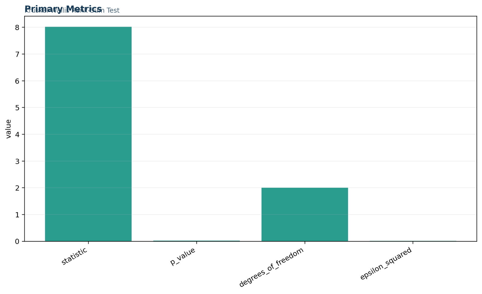
In this worked Kruskal Wallis test example, the outcome variable is G3 and the grouping variable is guardian. The three independent groups are father (n = 153), mother (n = 455), and other (n = 41). After pooling all 649 final-grade values into a single rank system and applying the tie correction, the Kruskal Wallis test produced H(2) = 8.0177 with p = 0.01815. This means the final-grade distributions are not all the same across the three guardian categories.
What does the Kruskal Wallis test measure?
An omnibus comparison of three or more independent groups using pooled ranks rather than raw means.
The Kruskal Wallis test, also written as the Kruskal-Wallis H test, compares whether three or more independent groups come from the same distribution. Instead of working directly with group means, the Kruskal Wallis test pools all observations together, ranks them from smallest to largest, and then asks whether the groups differ more in their average ranks than would be expected by chance.
This rank-based logic is why the Kruskal Wallis test is widely presented as the nonparametric alternative to one-way ANOVA. It is especially useful when the outcome is skewed, contains outliers, shows strong ceiling or floor effects, or is not comfortable under the usual normal-distribution assumptions. It is also a natural fit when the public explanation needs to focus on a broader comparison of group positions rather than only on arithmetic means.
Why the Kruskal Wallis test is used
People often search why Kruskal Wallis test is used or what does Kruskal Wallis test compare. The short answer is that the Kruskal Wallis test compares the location of groups in a shared rank distribution. If one group tends to contain higher values than another, that tendency shows up as a higher mean rank.
Because the method works with ranks, the Kruskal Wallis test can be more robust than ANOVA when raw values are awkwardly distributed. It still requires thoughtful interpretation, but it can answer the group-comparison question without relying on a strict normal-theory framework.
What the test does not do by itself
The Kruskal Wallis test is an omnibus test. That means it tells you whether at least one group differs, but it does not by itself identify which pairs differ. When the Kruskal Wallis test is significant, a follow-up procedure such as Dunn’s test or Conover test is usually needed for pairwise interpretation.
It also does not estimate a mean difference parameter in the way a t test does. Its main output is the H statistic, the p-value, and a rank-based interpretation.
Distribution difference versus median difference
A Kruskal Wallis test is often described as a test of medians, but that wording is only fully defensible when the group distributions have reasonably similar shapes. The formal null concerns the equality of distributions. If one group is more skewed or more variable than another, the test can become significant even when the sample medians appear close. For that reason, a strong public explanation combines the H statistic with box plots, medians, interquartile ranges, and group rank summaries.
This broader framing also connects naturally to box-plot interpretation, interquartile range, and five-number summaries. Those descriptive tools help reveal whether the significant result is mainly a location shift, a spread difference, or a more general distributional contrast.
Why ranks improve robustness
Ranks reduce the influence of unusually large or small raw observations because the procedure uses order rather than the original measurement distance. A very high value still receives a high rank, but it does not dominate the analysis merely because it is numerically far from the center. This makes the Kruskal Wallis test attractive for outcomes with skewness, ceiling effects, floor effects, or isolated outliers.
Robustness does not mean the data no longer matter. The group order, sample sizes, ties, and distribution shapes remain important. Ranking changes the scale of analysis; it does not remove the need for thoughtful design and interpretation.
The method is also a natural bridge between elementary descriptive work and formal hypothesis testing. Analysts often begin with descriptive statistics, five-number summaries, and box plots. The Kruskal Wallis test then formalizes what those summaries suggest by converting the full multi-group comparison into one coherent rank-based statistic.
When should you use the Kruskal Wallis test?
Choose the method when your design has one independent grouping variable and at least three independent groups.
A common query is when to use Kruskal Wallis test. The practical decision rule is simple: use the Kruskal Wallis test when you have one numeric or ordinal outcome, three or more independent groups, and a reason not to rely on ordinary one-way ANOVA assumptions.
Three or more groups
The method is built for comparisons like father, mother, and other guardian groups.
Independent observations
Each observation should belong to only one group with no repeated measurement across groups.
Rankable outcome
The response must be at least ordinal so that pooled ranking is meaningful.
Nonparametric preference
Use it when a rank-based analysis is preferred over a parametric ANOVA framework.
Need omnibus evidence
The Kruskal Wallis test is the first-stage overall comparison before pairwise follow-up.
A practical selection checklist
The Kruskal Wallis test is usually a strong choice when all five conditions are true: there is one categorical grouping variable, there are at least three independent groups, the outcome can be ordered, the research question is an omnibus comparison, and a parametric one-way ANOVA model is not preferred. If any one of those conditions fails, the analyst should reconsider the method before interpreting a p-value.
For example, three classrooms measured once each can fit an independent-group design, while the same classroom measured at three occasions does not. Three ordered treatment doses may also call for a trend-focused method rather than a general omnibus test. Method selection is strongest when it follows the research design rather than simply reacting to a normality test.
Situations that fit the Kruskal Wallis test well
Situations where another method fits better
Another reason the Kruskal Wallis test remains popular is interpretability across many applied fields. In education, health sciences, psychology, business, and quality-control studies, researchers frequently face data that are bounded, irregular, or clearly non-normal. In those settings, the Kruskal Wallis test offers a familiar and defensible way to compare several independent groups without forcing the analysis into a model that the raw data do not comfortably support.
Kruskal Wallis test assumptions
Nonparametric does not mean assumption-free. It means the assumptions are different and usually more flexible.
The Kruskal Wallis test assumptions are often easier to satisfy than ANOVA assumptions, but they still matter. The method requires independent observations, a grouping variable with independent categories, and an outcome that can be meaningfully ranked. It does not require strict normality, which is one reason the Kruskal Wallis test is so widely taught.
Independent groups
Each student in the example belongs to one guardian category only, so the design is independent rather than repeated or matched.
Ordered or numeric outcome
The outcome variable G3 is a final-grade score, so it can be ranked from lowest to highest without difficulty.
Pooled ranking across all groups
Every observation is ranked together in one shared pool. Group-specific ranks are not computed separately.
Distributional focus
The safest interpretation is in terms of group distributions and rank positions. When shapes are broadly similar, people often describe the result as a difference in typical level or central tendency.
Handling of ties
Because final grades repeat often, tied values are present. The Kruskal Wallis test therefore uses a tie correction to keep the H statistic properly calibrated.
Omnibus scope
The method tells you whether at least one group differs. It does not by itself identify the specific pairwise differences.
Independence is a design assumption
Independence cannot be repaired after the analysis by changing a software option. It comes from how the data were collected. If students are clustered within the same household, classroom, or school, their observations may be more alike than completely independent cases. In strongly clustered data, a multilevel or cluster-aware approach may be more appropriate than a simple Kruskal Wallis test.
Ties affect the reference statistic
Final grades are discrete and repeated, so tied observations are common in this example. Midranks ensure equal values receive the same average rank, and the tie correction adjusts the null variance used by the H statistic. Reporting the corrected result is important because an uncorrected H can slightly misstate the evidence when ties are numerous.
In teaching settings, one of the most helpful habits is to check assumptions before reading the p-value. Ask whether the groups are truly independent, whether the outcome can be ranked meaningfully, whether ties are present, and whether the question is really an omnibus multi-group question. When those pieces line up, the Kruskal Wallis test becomes much easier to defend and explain.
Null and alternative hypotheses
The Kruskal Wallis test is an omnibus test, so its hypotheses are global rather than pairwise.
Null hypothesis
H0: the father, mother, and other guardian groups share the same final-grade distribution.
Under this null, any rank differences across groups are attributable to random variation alone.
Alternative hypothesis
H1: at least one guardian group has a different final-grade distribution.
This does not specify which group differs; it only states that not all groups are alike.
G3 final grade
guardian
three independent groups
This hypothesis structure is why a significant Kruskal Wallis test naturally leads to follow-up pairwise procedures. Once the global null is rejected, the next statistical task is to identify where the differences lie.
That distinction between omnibus and pairwise inference is central to good statistical communication. A reader may be tempted to jump directly from a significant Kruskal Wallis test to a strong statement about one specific group contrast, but that step requires additional evidence. The omnibus result tells us the overall pattern is not flat; the post hoc stage tells us where the meaningful pairwise differences occur.
Kruskal Wallis test formula and tie correction
The H statistic is built from group rank sums and then adjusted for ties.
In this expression, N is the total sample size, k is the number of groups, Ri is the rank sum for group i, and ni is the size of group i. This gives the uncorrected Kruskal Wallis H statistic.
When ties exist, the Kruskal Wallis test divides the uncorrected statistic by the tie-correction factor. In this worked example, the tie correction is 0.9872190615, increasing the final H slightly from 7.9153 to 8.0177.
The formula is simple in appearance but conceptually rich. First, the Kruskal Wallis test discards the absolute scale long enough to replace raw values with pooled ranks. Second, it summarizes each group through its rank sum. Third, it rescales the overall contrast into the H statistic. Finally, because real datasets often contain repeated values, a tie correction is applied so that the test statistic is not understated or overstated.
Manual calculation sequence
Pool the scores
Combine all 649 G3 observations into one ordered list.
Assign midranks
Give tied grade values their average pooled rank.
Sum within groups
Calculate Ri for father, mother, and other.
Compute H
Insert rank sums and group sizes into the omnibus formula.
Correct ties
Divide by the tie-correction factor before finding the p-value.
This sequence explains why the Kruskal Wallis test is more than a black-box command. Every element of the final statistic can be traced back to the pooled ranks and group membership.
Exact calculation components
How the p-value is obtained
For moderate or large samples, the Kruskal Wallis test compares the H statistic to a chi-square reference distribution with k − 1 degrees of freedom. Here, with three groups, the reference distribution uses df = 2. The resulting p-value is 0.0181539.
The test also includes an effect-size summary, epsilon squared = 0.009315. That value indicates a small but nonzero group association. In other words, the result is statistically significant, but the overall magnitude of the guardian effect is modest.
Variables used in the worked example
A clean data dictionary helps readers see exactly what the Kruskal Wallis test is comparing.
| Variable | Role | Description |
|---|---|---|
| G3 | Outcome variable | Final grade score used as the ranked response in the Kruskal Wallis test. |
| guardian | Grouping variable | Independent group membership with categories father, mother, and other. |
| father | Group 1 | 153 observations; highest mean rank in the analysis. |
| mother | Group 2 | 455 observations; middle mean rank in the analysis. |
| other | Group 3 | 41 observations; lowest mean rank in the analysis. |
These descriptive statistics already hint at the eventual Kruskal Wallis test result. The father group has the highest raw mean, while the other group has the lowest. The rank-based analysis turns those descriptive differences into a formal inferential statement.
The value of listing the raw descriptive summaries alongside the rank results is that readers can see both layers of the story. On the original G3 scale, the differences are visible but not dramatic. On the rank scale, those same differences become organized into a clean omnibus comparison. That combination of descriptive and inferential detail makes the Kruskal Wallis test much easier to interpret responsibly.
Worked example: final grades across guardian groups
The full example shows how the Kruskal Wallis test translates descriptive differences into a formal statistical result.
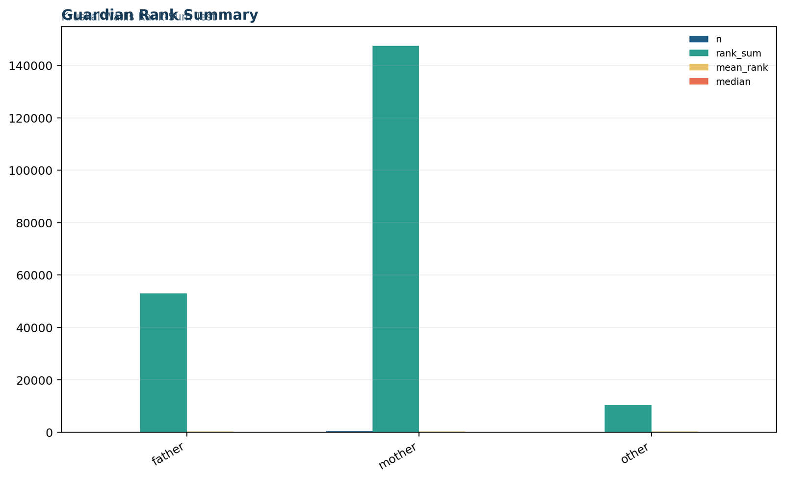
The worked Kruskal Wallis test example compares final-grade outcomes across the three guardian categories. Every G3 value is pooled, assigned a midrank where ties occur, and then aggregated within each group. The resulting group rank sums are 53,042 for father, 147,464 for mother, and 10,419 for other.
Dividing these rank sums by their group sizes gives the mean ranks: 346.68 for father, 324.10 for mother, and 254.12 for other. Because the father group sits highest and the other group sits lowest, the pooled-rank structure suggests that the father group generally occupies better final-grade positions within the combined sample.
The gap between father and mother mean ranks is about 22.58 rank units, whereas the gap between father and other is about 92.56. The mother-versus-other gap is about 69.97. These distances help readers anticipate which pairwise contrasts may be more influential, but they are not substitutes for adjusted post hoc p-values. The omnibus Kruskal Wallis test establishes that some difference exists; Dunn or Conover comparisons determine whether those specific gaps remain significant after multiplicity control.
It is also helpful to remember that the Kruskal Wallis test does not say every observation in the father group is high or every observation in the other group is low. Instead, it summarizes the overall direction of the pooled ranking pattern. That is a subtle but important point for public interpretation, especially when audiences might otherwise assume a stronger deterministic difference than the data justify.
What the rank pattern suggests
The Kruskal Wallis test is sensitive to the relative ordering of observations, not only to the arithmetic difference in group means. In this example, the rank pattern shows a fairly clear ordering: father highest, mother middle, other lowest. This does not mean every student in one group scores above every student in another, but it does mean the center of the rank distribution tends to shift across groups.
Because the other guardian group is also the smallest group, it is especially important that the interpretation remain rank-based rather than overly literal about group means alone.
Observed omnibus result
The tie-corrected Kruskal Wallis result supports a statistically significant group difference.
At the conventional 0.05 significance level, the null hypothesis of equal guardian-group distributions is rejected. This is the point where a post hoc procedure becomes valuable for pairwise explanation.
Exact Kruskal Wallis test results table
The core values are easiest to interpret when placed in one complete summary table.
| Metric | Value | Interpretation |
|---|---|---|
| father rank sum | 53,042 | Total pooled ranks assigned to the father group. |
| mother rank sum | 147,464 | Total pooled ranks assigned to the mother group. |
| other rank sum | 10,419 | Total pooled ranks assigned to the other group. |
| father mean rank | 346.6797 | Highest mean rank among the three guardian categories. |
| mother mean rank | 324.0967 | Middle mean rank. |
| other mean rank | 254.1220 | Lowest mean rank. |
| Tie-corrected H | 8.0177395916 | Final Kruskal Wallis test statistic. |
| Degrees of freedom | 2 | Based on k − 1 for three groups. |
| p-value | 0.0181539013 | Evidence that the distributions are not all equal. |
| Epsilon squared | 0.0093153864 | Small omnibus effect size. |
What the table means in plain language
The Kruskal Wallis test table shows that the groups are not identical in their rank distributions. The difference is statistically significant but not large in effect-size terms. That is a useful and honest summary: guardian status appears to be associated with final-grade ranking, but the overall strength of the association is modest.
How to interpret the Kruskal Wallis test
Good interpretation combines the omnibus result, the rank pattern, and the need for follow-up testing.
Many readers ask what is the test statistic for Kruskal Wallis or how to interpret Kruskal Wallis test results. A complete interpretation should mention the H statistic, the p-value, the direction of rank differences, and whether pairwise testing is needed.
Statistical decision
Because p = 0.01815 is below 0.05, the omnibus null is rejected. The guardian groups do not all share the same final-grade distribution.
Direction of the rank pattern
The father group has the highest mean rank, the mother group is intermediate, and the other group has the lowest mean rank. This suggests better relative grade positions in the father group than in the other group.
What comes next
The Kruskal Wallis test alone cannot identify the significant pairs. A post hoc method such as Dunn’s test is the standard next step.
Publicly reported interpretation can therefore be framed as follows: a Kruskal Wallis test showed that final grades differ across guardian categories, with the father group tending to occupy higher rank positions and the other group lower rank positions. However, additional pairwise testing is needed to confirm which specific group contrasts drive the omnibus result.
Statistical significance
The p-value addresses whether the observed rank separation is unlikely under the global null hypothesis. Here it is below .05, so the omnibus evidence is statistically significant.
Practical magnitude
Epsilon squared addresses how much of the rank variability is associated with guardian grouping. The value of .0093 is small, so the practical effect should be described as modest rather than dramatic.
This distinction is essential because large samples can detect relatively subtle patterns. A careful results section therefore presents both the inferential decision and the effect-size context rather than allowing the p-value to carry the entire interpretation.
The effect-size estimate helps refine that message. With epsilon squared = 0.009315, the omnibus effect is small. So the result is statistically significant, but it should not be exaggerated into a claim of a huge or overwhelming guardian effect. That balance between significance and magnitude is one of the most important parts of good statistical writing.
Kruskal Wallis test in Python: chart-by-chart interpretation
The Python figures move from the omnibus summary to the group-rank structure and final verified conclusion.
Searchers often want Kruskal Wallis test in Python examples that do more than print a single statistic. The chart set below explains the logic of the Kruskal Wallis test visually while keeping the same full boxed-figure format used in the permanent site design.
Python is particularly good for teaching the Kruskal Wallis test because every step can be scripted transparently. The data can be imported, ranks can be checked directly, group summaries can be calculated in a reproducible workflow, and the final H statistic can be verified in code. That transparency is one reason Python examples are valuable for public readers who want both the result and the reasoning behind it.
Python chart 1: primary metrics
This opening figure acts as the dashboard for the entire Kruskal Wallis test result. It summarizes the tie-corrected H = 8.0177, the p-value = 0.01815, the small omnibus effect size ε² = 0.00932, and the overall sample structure. The chart shows immediately that the result is statistically significant but modest in magnitude.
Python chart 2: guardian rank summary
This figure is the clearest visual explanation of the Kruskal Wallis test outcome. The mean ranks are 346.68 for father, 324.10 for mother, and 254.12 for other. Because the test is rank-based, this ordering directly explains why the omnibus statistic becomes significant.
Python chart 3: ranked observations
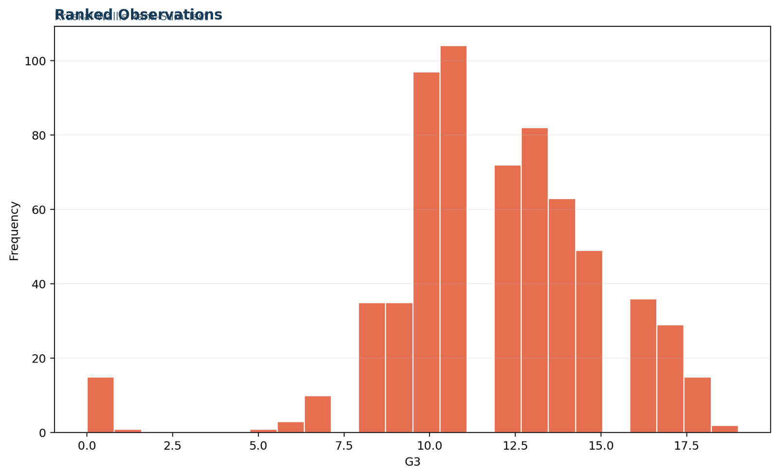
The ranked-observations chart reminds readers that the Kruskal Wallis test uses pooled rank positions, not the original values alone. By plotting or summarizing the ranked records, the figure reveals how one group can accumulate a larger share of higher rank positions than another.
Python chart 4: rank quantiles
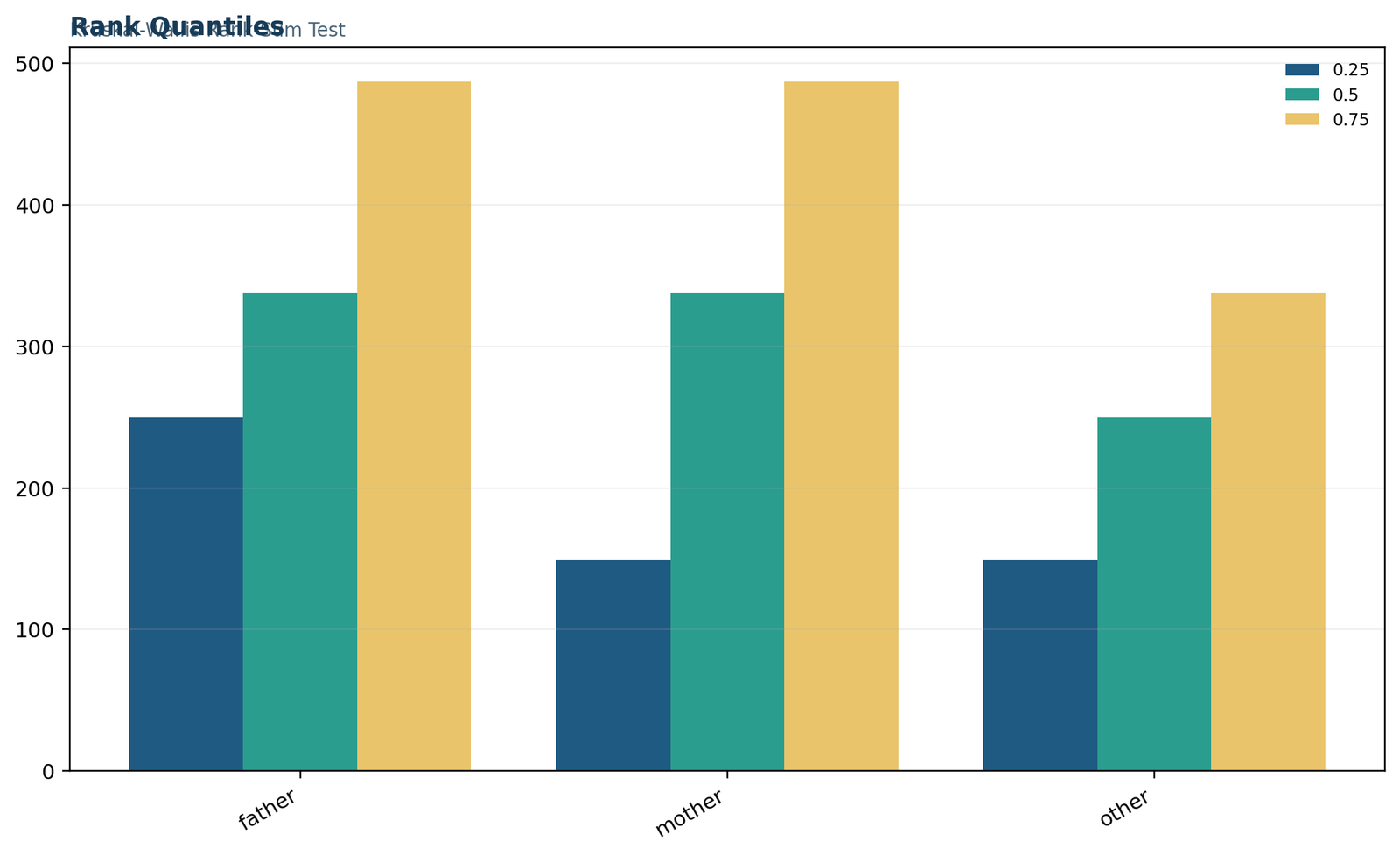
This chart adds distributional detail by showing where group ranks sit across the lower, middle, and upper portions of the pooled rank scale. The father group tends to sit higher, the mother group occupies the middle range, and the other group is lower, consistent with the mean-rank summary.
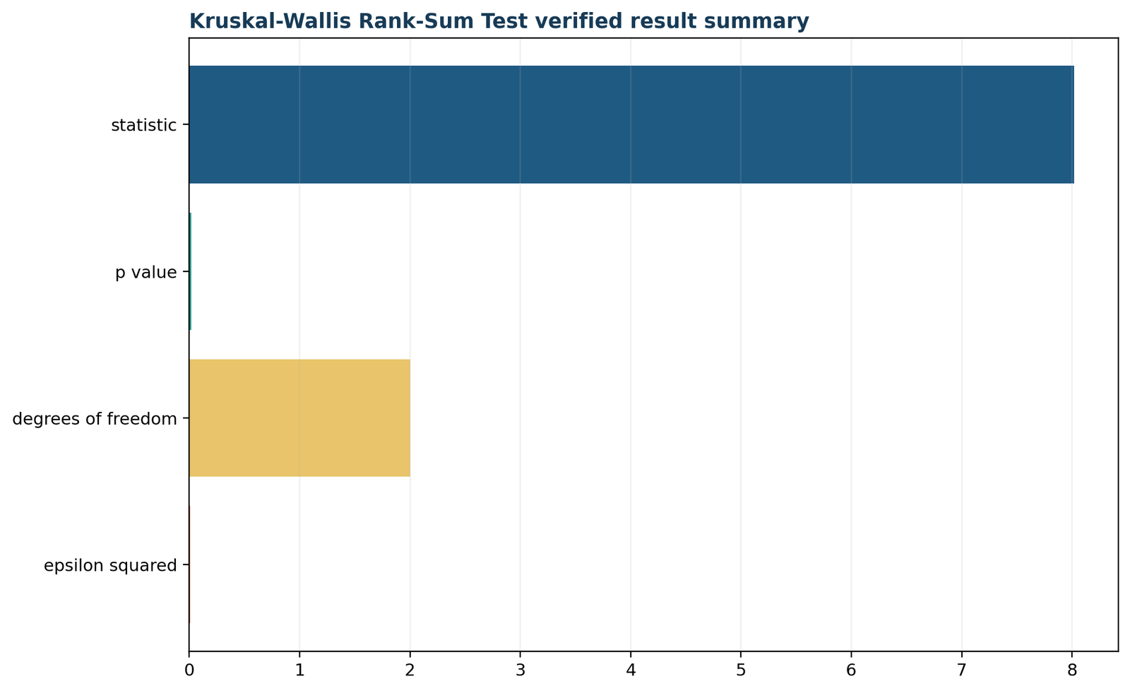
Python chart 5: verified result summary
The closing summary panel condenses the whole Kruskal Wallis test story into one public conclusion: the guardian groups differ overall, the effect is modest, and post hoc testing is the logical next step for pairwise detail.
Kruskal Wallis test in R: chart-by-chart interpretation
The R analysis reproduces the same rank-based message and strengthens reproducibility.
The Kruskal Wallis test in R is widely used in teaching, biostatistics, and social-science applications. The R figure set confirms that the result does not depend on one software platform alone. When Python and R converge on the same H statistic, p-value, and rank ordering, the interpretation becomes more stable and trustworthy.
R is also a strong environment for the Kruskal Wallis test because it supports not only the omnibus analysis but also rich post hoc extensions, diagnostics, tables, and graphics. For readers building an end-to-end workflow, that makes R a practical bridge from a first omnibus finding to a full analysis report.
R chart 1: primary metrics
The first R chart reproduces the key numerical results of the Kruskal Wallis test. It shows that the omnibus group comparison is significant and ties the p-value directly to the tie-corrected H statistic.
R chart 2: guardian rank summary
This chart again places the group mean ranks side by side. The consistency of the father > mother > other ordering is the central visual insight of the whole Kruskal Wallis test example.
R chart 3: ranked observations
The R ranked-observations figure shows how the pooled ranking process transforms raw G3 values into the material used by the H statistic. This is especially useful for public readers who want to understand why rank-based tests can be more robust than mean-based methods.
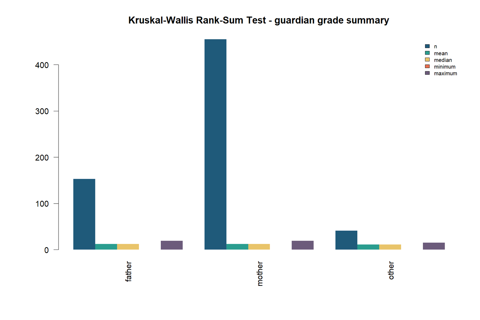
R chart 4: guardian grade summary
This chart reconnects the rank-based analysis with the original grade scale. The father group has the highest mean raw G3 value, the mother group is slightly lower, and the other group is lowest. That raw-data story complements the rank-based omnibus result rather than replacing it.
R chart 5: verified result summary
The final R figure restates the essential finding: the Kruskal Wallis test identifies a statistically significant difference across guardian groups, but further pairwise analysis is needed to specify which contrasts are responsible.
Kruskal Wallis test in SPSS
SPSS users reach the same inferential conclusion even though the menus and tables look different.
How to conduct a Kruskal Wallis test in SPSS
The SPSS workflow begins by placing G3 in the test-variable field and guardian in the grouping field, defining the three guardian codes, and requesting the independent-samples nonparametric comparison. The resulting output should be checked for group counts, rank summaries, the H statistic, degrees of freedom, and the significance value. When post hoc comparisons are produced, the adjustment method must be stated clearly in the written report.
SPSS may display the procedure through different interfaces depending on version and menu choice, but the statistical logic remains the same. A correct public explanation should not depend on a particular screenshot; it should explain the pooled ranks, omnibus decision, and follow-up requirement.
SPSS interpretation points
In SPSS, the Kruskal Wallis test still compares pooled ranks across independent groups. The important pieces to read are the group structure, the test statistic, the degrees of freedom, and the p-value. The public interpretation stays the same: this is an omnibus nonparametric comparison, not a built-in pairwise answer.
If the omnibus result is significant, SPSS users should either run or report an appropriate post hoc follow-up. It is also useful to pair the inferential table with group descriptive summaries such as medians, interquartile ranges, and mean ranks.
SPSS conclusion for this example
The SPSS output agrees with the Python and R results: H(2) = 8.0177, p = 0.01815. This means the guardian groups differ overall in their final-grade rank distributions. The software platform changes the display, but not the substantive meaning.
Kruskal Wallis test in Excel
The workbook makes every ranking and tie-correction step visible and auditable.
Searchers often ask can you do a Kruskal Wallis test in Excel or how to calculate Kruskal Wallis test in Excel. The workbook used here shows that the answer is yes. Excel is especially valuable because it exposes every intermediate step: raw inputs, pooled ranks, rank sums, tie correction, final H, and the reporting cross-check.
| Workbook sheet | Purpose in the Kruskal Wallis workflow |
|---|---|
| Guide | Documents the design, variables, formula, alpha level, and workbook scope. |
| Data_Input | Stores the unchanged G3 and guardian values used in the analysis. |
| Working | Shows pooled midranks and tie contributions for every row. |
| Calculations | Displays group rank sums, mean ranks, uncorrected H, tie correction, corrected H, and p-value. |
| Diagnostics | Lists key methodological checks such as pooled ranking and tie handling. |
| Reporting | Cross-checks workbook outputs against the verified reference results. |
What must be formula-driven
A reliable Excel implementation should calculate ranks from the raw G3 column, summarize rank sums with group conditions, derive H from the formula, and calculate the tie correction from the observed frequency of repeated grades. Hard-coding the final statistic removes the main educational and audit value of the workbook.
How to validate the workbook
The strongest check is cross-software agreement. The Excel result should match Python, R, and SPSS for H, df, and p-value. In this analysis, the workbook and verified reference agree exactly to displayed precision, which confirms that the ranking and tie formulas are functioning correctly.
That transparency matters for SEO-style educational content too, because many readers specifically want to know how to do a Kruskal Wallis test in Excel. A workbook that exposes every intermediate piece is far more useful than a black-box calculator result. It helps students, researchers, and auditors verify that the rank sums, tie correction, and final statistic all align correctly.
How to report Kruskal Wallis test results
Readers often need a polished reporting model rather than only a software table.
Reporting quality matters because many public posts stop after printing a p-value. A better Kruskal Wallis test report tells readers what was compared, what statistic was obtained, whether the result was significant, what direction the group ranks took, and whether post hoc analysis is needed. That richer narrative is what transforms a software output into a real explanation.
Reporting structure for a significant result
A complete report follows a logical sequence: identify the nonparametric omnibus method, name the outcome and grouping variable, report H and df, state the p-value, add an effect size, describe the rank direction, and explain that post hoc testing is required. This structure answers both statistical and substantive questions without overstating what the omnibus analysis proves.
For a non-significant analysis, the same structure can be used, but the conclusion should say that the evidence was insufficient to detect distributional differences. The wording should avoid claiming that all populations are proven identical.
APA-style example
A Kruskal Wallis test showed a statistically significant difference in final grades across guardian categories, H(2) = 8.02, p = .018, ε2 = .009. Mean ranks were highest for the father group (346.68), followed by the mother group (324.10), and lowest for the other group (254.12). These results indicate that final-grade distributions differ across guardian categories. Follow-up pairwise tests are needed to determine which specific group contrasts are significant.
What to include
- Name the Kruskal Wallis test explicitly.
- Report H, degrees of freedom, and p-value.
- Mention a rank-based direction statement using mean ranks or medians.
- Include effect size when available.
- State whether follow-up pairwise testing is needed.
What to avoid
- Do not treat the omnibus test as if it automatically identifies the significant pairs.
- Do not call it a test of means only.
- Do not ignore the role of ties when they are clearly present.
- Do not forget that the safest interpretation is distributional rather than purely parametric.
Post hoc testing and related methods
A significant Kruskal Wallis result is often the beginning of the explanation, not the end of it.
| Method | Best use | How it relates to the Kruskal Wallis test |
|---|---|---|
| Dunn’s test | Post hoc pairwise comparisons | Standard follow-up after a significant Kruskal Wallis test. |
| Conover test | Post hoc pairwise comparisons | Alternative follow-up method often used after Kruskal Wallis. |
| Friedman test | Repeated-measures rank comparison | Used instead of Kruskal Wallis when the design is not independent. |
| Jonckheere–Terpstra test | Ordered trend alternative | More focused than Kruskal Wallis when the groups have a natural order. |
| One-way ANOVA | Parametric independent-group comparison | The Kruskal Wallis test is the common nonparametric alternative. |
Readers often search post hoc test for Kruskal Wallis or Kruskal Wallis test post hoc. In practice, that means using the omnibus result as a gateway to pairwise procedures such as Dunn or Conover. Because the current chart set focuses on the omnibus test, the pairwise step is referenced conceptually rather than reported as part of the main result table.
Multiplicity adjustment
Three groups create three pairwise comparisons. Testing each pair at .05 without adjustment would inflate the familywise Type I error rate. Procedures such as Holm or Bonferroni modify the decision thresholds so that the collection of pairwise conclusions remains controlled. Holm is often attractive because it is less conservative than simple Bonferroni while retaining familywise protection.
Choosing Dunn or Conover
Dunn’s test is the most widely recognized rank-based follow-up after a significant Kruskal Wallis test. Conover’s method is another valid alternative and may differ in power. The chosen method should be specified before reporting the pairwise results, and adjusted p-values should always be distinguished from unadjusted values.
That sequence mirrors good analytical practice. First answer the overall question with the Kruskal Wallis test. Then, only if the omnibus result is significant, move to multiple-comparison procedures that control the error rate appropriately. This protects the analysis from unnecessary pairwise testing and keeps the interpretation disciplined.
Downloads
These links provide the supporting materials for the complete worked example.
Python reportDetailed Python output and interpretation for the Kruskal Wallis test.Open report
R reportR output for the same omnibus rank-based analysis.Open report
SPSS outputSPSS companion output for the worked example.Open report
Excel workbookAuditable workbook with pooled ranks, tie correction, and reporting cross-checks.Open workbook
Frequently asked questions about the Kruskal Wallis test
Short answers to common public questions about the method, its use, and its interpretation.
What is the Kruskal Wallis test?
The Kruskal Wallis test is a nonparametric method for comparing three or more independent groups using pooled ranks.
When should I use the Kruskal Wallis test?
Use the Kruskal Wallis test when you have three or more independent groups and want a nonparametric alternative to one-way ANOVA.
What does the Kruskal Wallis test compare?
It compares whether independent groups share the same overall distribution, as reflected in their pooled rank positions.
What was the H statistic in this example?
The tie-corrected Kruskal Wallis test statistic was H = 8.0177395916.
What was the p-value in this example?
The p-value was 0.0181539013.
Was the Kruskal Wallis test significant?
Yes. The p-value is below 0.05, so the omnibus null hypothesis of equal group distributions is rejected.
Which group had the highest mean rank?
The father group had the highest mean rank at 346.68.
Which group had the lowest mean rank?
The other guardian group had the lowest mean rank at 254.12.
Does the Kruskal Wallis test require normality?
No. The Kruskal Wallis test is rank-based and does not require a normal distribution.
Does the Kruskal Wallis test identify which pairs differ?
No. It is an omnibus test, so a separate post hoc procedure is needed for pairwise comparisons.
What post hoc test can follow a Kruskal Wallis test?
Common follow-up choices include Dunn’s test and Conover test.
What effect size was reported?
The omnibus effect size was epsilon squared = 0.009315, which is small.
What are the group sizes in the worked example?
The sample sizes are father = 153, mother = 455, and other = 41.
Why was a tie correction needed?
Many final-grade values repeat, so the Kruskal Wallis test uses a tie correction to adjust the H statistic appropriately.
Can the Kruskal Wallis test be done in Excel?
Yes. The workbook linked in this guide shows every step of the calculation, including pooled ranks and tie correction.
Can the Kruskal Wallis test be done in R and Python?
Yes. This guide includes matched Python and R chart sections along with downloadable reports.
How should Kruskal Wallis results be reported?
Report the H statistic, degrees of freedom, p-value, a direction statement using ranks or medians, and note whether follow-up pairwise tests are needed.
What is the main conclusion of this worked example?
The guardian groups differ significantly in their final-grade rank distributions, with the father group tending to rank highest and the other group lowest.
Is the Kruskal Wallis test a test of medians?
It is more accurately a test of distributional equality. It can be interpreted as a median or location comparison when group distributions have similar shapes.
How many groups can the Kruskal Wallis test compare?
It can compare three or more independent groups. There is no fixed upper limit, although interpretation and post hoc complexity increase as the number of groups grows.
What happens if the groups have unequal sample sizes?
Unequal group sizes are allowed. The formula explicitly accounts for each group size through the Ri2/ni terms.
Why should effect size be reported with the p-value?
The p-value describes statistical evidence, while effect size describes magnitude. Reporting both prevents a small but significant pattern from being presented as a large practical effect.
Can Kruskal Wallis results be followed by box plots?
Yes. Box plots are useful for showing medians, interquartile ranges, outliers, and distribution shape alongside the rank-based omnibus result.
Is the Kruskal Wallis test the same as one-way ANOVA?
No. One-way ANOVA is a parametric mean-based procedure, whereas the Kruskal Wallis test is a nonparametric rank-based omnibus test.
Why is the Kruskal Wallis test often called an omnibus test?
It is called omnibus because it evaluates the overall null that all groups are alike, rather than a single pairwise contrast.
Can the Kruskal Wallis test handle tied values?
Yes. Tied values are handled through midranks and a tie-correction factor, which is why the method works well with repeated score values.