
Bowker's Test of Symmetry: Formula, Calculator, Example, Python, R, SPSS and Excel Guide
Bowker's Test of Symmetry, also called the McNemar-Bowker test, evaluates whether paired categorical transitions are symmetric in a square contingency table. This complete guide explains the Bowker test formula, hypotheses, assumptions, degrees of freedom, calculator logic, pairwise contributions, exact McNemar follow-ups, APA reporting, seven shared separate Python and R charts, SPSS and Excel workflows, and a worked analysis of 649 paired student grades.
3 × 3 square table
Bowker χ² = 62.1611
p = 3.176 × 10⁻¹⁴
Bowker's Test of Symmetry Model Overview
Bowker's Test of Symmetry is a chi-square procedure for paired nominal or ordinal categorical data. Each observational unit is measured twice using the same category set, and the resulting counts form a square k × k contingency table. The test compares every off-diagonal transition count with its reverse transition count.
What Question Does Bowker's Test Answer?
The method asks whether movement between categories is directionally balanced. For every pair of categories i and j, the transition count from i before to j after is compared with the reverse count from j before to i after.
Worked Research Scenario
The same 649 students have a before measurement from G1 and an after measurement from G3. Both grades are converted to the same three categories: Low = 0–9, Medium = 10–13, and High = 14 or above. Bowker's Test asks whether transitions between these grade bands are symmetric.
Why the Test Uses Only Off-Diagonal Counts
Diagonal cells represent students who stayed in the same category. They describe agreement and stability but provide no evidence about directional imbalance. Bowker's Test is built from discordant off-diagonal pairs such as Low→Medium versus Medium→Low.
Bowker Test Formula
The observed statistic is 62.161111. The Low↔Medium pair contributes 40.111111; the Medium↔High pair contributes 22.050000; and the Low↔High pair contributes zero because no students moved directly between those two bands.
Current Worked Result
The analysis contains 649 complete pairs. The effective degrees of freedom are 2, and the p-value is 3.17604193e-14. The null hypothesis of symmetry is rejected. The observed changes are strongly directional, with 130 upward transitions and 31 downward transitions.
Quick Answer: Bowker's Test of Symmetry Result
Test Summary
- Before variable: G1 grade band
- After variable: G3 grade band
- Categories: Low, Medium, High
- Alternative: at least one asymmetric reverse pair
- Decision: reject symmetry
Substantive Meaning
- Upward transitions: 130
- Downward transitions: 31
- Stable diagonal cases: 488
- Agreement rate: 75.19%
- Directional asymmetry index: 0.6149
Table of Contents
- What is Bowker's Test of Symmetry?
- Research question, hypotheses and paired design
- When to use the McNemar-Bowker test
- Bowker test formula and calculation
- Variables and data dictionary
- Complete worked results
- Pairwise contributions and follow-up tests
- Bowker versus McNemar, Stuart-Maxwell and kappa
- Bowker test calculator steps
- Seven Python chart interpretations
- Seven R charts with paired explanations
- Assumptions, diagnostics and limitations
- Python, R, SPSS and Excel workflows
- Expandable software code
- Advanced Bowker test topics
- APA reporting for Bowker's Test
- Common mistakes and corrections
- Reports and worked Excel download
- Related Salar Cafe guides
- Frequently asked questions
- Conclusion
What Is Bowker's Test of Symmetry?
Bowker's Test of Symmetry is the multi-category extension of McNemar's test. McNemar's test handles a paired 2 × 2 table; Bowker's Test extends the same reverse-cell logic to a square table with three or more categories.
Paired Square Contingency Table
A valid Bowker table uses the same category labels in the same order for the before and after measurements. Rows represent the first measurement and columns represent the second. Cell nij counts observations that started in category i and ended in category j.
Symmetry Around the Main Diagonal
A perfectly symmetric table has nij = nji for every off-diagonal pair. Symmetry does not require the diagonal cells to be equal, and it does not require a particular agreement rate. It requires each directional flow to be balanced by the reverse flow.
Directional Interpretation
For ordered grade bands, Low→Medium and Medium→High are upward movements. Medium→Low and High→Medium are downward movements. Bowker's Test is significant because the observed reverse-pair differences—57 for Low↔Medium and 42 for Medium↔High—are much larger than expected under symmetry.
McNemar-Bowker Test Name
The phrase McNemar-Bowker test emphasizes that Bowker's procedure generalizes McNemar's paired binary test. The terms Bowker test, Bowker's test of symmetry, and McNemar-Bowker test of symmetry normally refer to the same square-table symmetry procedure.
What Bowker's Test Does Not Measure
The test does not estimate agreement, reliability, association strength, or causal improvement. A table can have high diagonal agreement but still show asymmetric changes among the discordant cases. Conversely, a table can have low agreement with balanced directional transitions and therefore fail to reject symmetry.
Research Question, Hypotheses and Paired Data Design
Research Question
Are the paired transitions between G1 and G3 grade bands directionally symmetric, or do students move between grade bands more often in one direction than in the reverse direction?
Null Hypothesis
Alternative Hypothesis
Why the Observations Are Paired
G1 and G3 belong to the same student. Treating the two marginal distributions as independent samples would discard the within-student transition information. Bowker's Test retains the paired structure by analysing the complete square table.
Why the Same Categories Must Be Used
Symmetry is defined around the main diagonal. If the before and after variables use different labels, cutpoints, or category order, cell nij does not have a meaningful reverse partner nji. The same grade-band definitions are therefore applied to both G1 and G3.
When to Use the McNemar-Bowker Test
Use Bowker's Test When
- The same observational units are measured twice.
- Both measurements are categorical.
- The same categories are used at both occasions.
- The table is square.
- There are three or more categories.
- The question concerns directional symmetry.
- Each paired observation belongs to one cell.
- The off-diagonal counts are adequate for the chi-square approximation.
Choose Another Method When
- The two samples are independent rather than paired.
- The table is rectangular rather than square.
- There are only two categories and ordinary McNemar is sufficient.
- The main question is marginal homogeneity rather than full symmetry.
- Agreement or reliability is the primary target.
- Covariate adjustment is required.
- Repeated measurements exceed two occasions.
- Discordant pair totals are extremely sparse.
Bowker Test for Nominal and Ordinal Categories
The test can be used with nominal categories because it compares matched labels, but ordered categories provide additional directional meaning. With Low, Medium, and High, the positive differences can be interpreted as upward movement. The chi-square calculation itself does not use the numerical distance between categories.
Bowker Versus Independent-Sample Chi-Square
An independent-sample chi-square test assumes that the before and after counts come from unrelated observations. That assumption is false when the same students are measured twice. Bowker's Test uses the paired transition table and is the appropriate symmetry procedure.
More Than Two Time Points
Bowker's Test compares two categorical measurements. A study with three or more occasions requires a repeated categorical model, generalized estimating equations, a marginal model, or planned pairwise analyses with multiplicity control.
Bowker Test Formula and Step-by-Step Calculation
Step 1: Create the Paired Square Table
| Before G1 | After Low | After Medium | After High | Before total |
|---|---|---|---|---|
| Low | 88 | 69 | 0 | 157 |
| Medium | 12 | 267 | 61 | 340 |
| High | 0 | 19 | 133 | 152 |
| After total | 100 | 355 | 194 | 649 |
Step 2: Identify Reverse Off-Diagonal Pairs
Difference = 57; discordant pair total = 81.
No discordant information for this pair.
Difference = 42; discordant pair total = 80.
Step 3: Calculate Each Pair Contribution
The Low↔High pair has a denominator of zero. It contributes no chi-square information and is excluded from the effective degrees of freedom used by the published Python and R reports.
Step 4: Sum the Pair Contributions
Step 5: Determine Degrees of Freedom
The nominal maximum for three categories is:
Because the Low↔High pair contains no discordant observations, the published workflow uses two informative reverse pairs and therefore an effective df of 2.
Step 6: Calculate the P-Value
Step 7: Make the Decision
Because the p-value is far below α = .05, reject H0. The paired transition table is directionally asymmetric.
Step 8: Interpret the Direction
The global statistic does not identify direction by itself. Direction comes from the signed pair differences: 69 Low→Medium versus 12 Medium→Low, and 61 Medium→High versus 19 High→Medium. Both informative pairs favour upward movement.
Variables and Data Dictionary
| Variable | Role | Original scale | Analysis coding | Valid N | Meaning |
|---|---|---|---|---|---|
| G1 | Before measurement | First-period grade, 0–19 | Low 0–9; Medium 10–13; High 14+ | 649 | Defines the row category. |
| G3 | After measurement | Final grade, 0–19 | Low 0–9; Medium 10–13; High 14+ | 649 | Defines the column category. |
| Student record | Paired observational unit | One row per student | One before-after category pair | 649 | Preserves within-student dependence. |
Before and After Marginal Distributions
| Grade band | Before count | Before percent | After count | After percent | After − before |
|---|---|---|---|---|---|
| Low | 157 | 24.1911% | 100 | 15.4083% | −57 |
| Medium | 340 | 52.3883% | 355 | 54.6995% | +15 |
| High | 152 | 23.4206% | 194 | 29.8921% | +42 |
Transition Percentages Within Each Before Category
| Before category | Stayed Low | Moved/Stayed Medium | Moved/Stayed High | Row total |
|---|---|---|---|---|
| Low | 56.1% | 43.9% | 0.0% | 157 |
| Medium | 3.5% | 78.5% | 17.9% | 340 |
| High | 0.0% | 12.5% | 87.5% | 152 |
Complete Bowker's Test of Symmetry Results
Sum of reverse-pair contributions
Two informative discordant pairs
Asymptotic chi-square reference
488 unchanged pairs
Changed grade bands
Net directional imbalance
Primary Bowker Test Result
| Test | Statistic | Degrees of freedom | P-value | Decision at .05 |
|---|---|---|---|---|
| Bowker's Test of Symmetry | 62.161111111 | 2 | 3.17604193e-14 | Reject symmetry |
Directional Transition Summary
Upward Movement
130
80.7% of changed cases moved to a higher grade band. Upward transitions were 69 Low→Medium and 61 Medium→High.
Downward Movement
31
19.3% of changed cases moved to a lower grade band. Downward transitions were 12 Medium→Low and 19 High→Medium.
Net Directional Change
Agreement and Stability
488 students remained in the same grade band, giving a simple diagonal agreement rate of 75.19%. The unweighted Cohen's κ is 0.591; linear-weighted κ is 0.653; and quadratic-weighted κ is 0.734. These agreement measures are descriptive companions, not components of Bowker's Test.
Marginal Interpretation
The Low category decreased from 157 to 100 students. Medium increased from 340 to 355, and High increased from 152 to 194. These marginal changes are consistent with the directional transition counts, although Bowker's Test evaluates the stronger condition of complete off-diagonal symmetry.
Pairwise Contributions and Exact McNemar Follow-Up Tests
The global Bowker statistic indicates that at least one reverse transition pair is asymmetric. Pair-level contributions identify which category comparisons create the result. Exact McNemar tests can then evaluate each informative reverse pair, with multiplicity control when the follow-ups are confirmatory.
| Category pair | i→j | j→i | Discordant total | Signed difference | Bowker contribution | Contribution share | Exact McNemar p |
|---|---|---|---|---|---|---|---|
| Low ↔ Medium | 69 | 12 | 81 | +57 | 40.111111 | 64.53% | 7.03300083e-11 |
| Low ↔ High | 0 | 0 | 0 | 0 | 0.000000 | 0.00% | Not estimable |
| Medium ↔ High | 61 | 19 | 80 | +42 | 22.050000 | 35.47% | 2.73186992e-06 |
Low Versus Medium
The Low↔Medium pair contributes 64.53% of the global statistic. There were 69 Low→Medium transitions and 12 Medium→Low transitions. The exact two-sided McNemar p-value is 7.03300083e-11, showing a strong directional imbalance toward Medium.
Medium Versus High
The Medium↔High pair contributes 35.47% of the statistic. There were 61 Medium→High transitions and 19 High→Medium transitions. The exact McNemar p-value is 2.73186992e-06, again favouring the upward direction.
Low Versus High
No students moved directly from Low to High or from High to Low. This pair contains no discordant information, contributes zero to the test statistic, and cannot support a pairwise McNemar calculation.
Multiplicity Adjustment
With two informative follow-up comparisons, a Bonferroni-adjusted alpha is .025. Both pairwise exact p-values remain far below that threshold. A Holm procedure leads to the same substantive conclusion.
Bowker Test Versus McNemar, Stuart-Maxwell and Kappa
Tests every reverse off-diagonal pair in a square table.
Tests symmetry for one paired binary 2 × 2 table.
Tests equality of the before and after marginal distributions.
Measures agreement beyond chance rather than directional symmetry.
Numerical Comparison for the Worked Table
| Procedure or measure | Statistic/value | df | P-value | Question answered |
|---|---|---|---|---|
| Bowker symmetry, effective df | 62.161111 | 2 | 3.17604193e-14 | Are all reverse transition pairs balanced? |
| Bowker symmetry, nominal df convention | 62.161111 | 3 | 2.02960250e-13 | Same statistic with nominal maximum df retained. |
| Stuart-Maxwell marginal homogeneity | 62.161111 | 2 | 3.17604193e-14 | Are before and after marginal proportions equal? |
| Simple agreement | 0.751926 | — | — | What proportion stayed in the same category? |
| Unweighted Cohen's κ | 0.590742 | — | — | How much exact agreement exceeds chance? |
| Linear-weighted κ | 0.652827 | — | — | How much ordered agreement exceeds chance with partial credit? |
| Quadratic-weighted κ | 0.733641 | — | — | How much ordered agreement exceeds chance with stronger near-match credit? |
Bowker Versus McNemar
McNemar's test is the 2 × 2 special case. With three categories, a single McNemar test cannot evaluate complete table symmetry. Bowker's Test combines all informative reverse pairs into one global statistic.
Bowker Versus Stuart-Maxwell
Bowker symmetry is a stronger condition than marginal homogeneity. Symmetry implies equal margins, but equal margins do not necessarily imply pairwise symmetry. In this particular table, the zero Low↔High pair makes the Stuart-Maxwell statistic numerically equal to the effective-df Bowker statistic. This equality is specific to the observed structure and should not be assumed generally.
Bowker Versus Cohen's Kappa
Kappa answers whether paired categories agree beyond chance. Bowker answers whether disagreements are directionally balanced. The table has a substantial diagonal agreement rate and moderate-to-strong kappa values, yet Bowker's Test strongly rejects symmetry because the discordant cases overwhelmingly move upward.
Bowker Versus an Independent Chi-Square Test
An ordinary independent chi-square table ignores the pairing of G1 and G3. It cannot distinguish whether a particular student moved from Low to Medium or another student moved in the reverse direction. Bowker's Test retains this within-student transition information.
Bowker Test Calculator: Step-by-Step Workflow
A reliable Bowker test calculator needs a square paired table, identical category labels on both axes, the chi-square formula, a rule for zero-discordance pairs, and a transparent degrees-of-freedom convention.
Calculator Inputs
| Input | Worked value | Validation rule |
|---|---|---|
| Number of categories | 3 | Rows and columns must use the same three labels. |
| Paired table | [[88,69,0],[12,267,61],[0,19,133]] | All entries must be nonnegative counts. |
| Complete pairs | 649 | Table total must equal the number of valid paired records. |
| Alpha | .05 | Select before analysis. |
| Zero-pair rule | Exclude from effective df | Low↔High has zero discordant total. |
Calculator Step 1: Check That the Table Is Square
A 3 × 3 table is valid because the same Low, Medium, and High categories appear on both axes. A 3 × 4 table does not have a complete set of reverse cells and cannot be analysed with the standard Bowker formula.
Calculator Step 2: Ignore the Diagonal in the Test Statistic
The diagonal counts 88, 267, and 133 describe category stability. They are not included in the numerator or denominator of the symmetry statistic.
Calculator Step 3: Calculate Each Reverse-Pair Term
For every i < j, calculate (nij − nji)²/(nij + nji). The worked informative terms are 40.111111 and 22.050000.
Calculator Step 4: Handle a Zero Pair Correctly
When nij + nji = 0, the expression is 0/0. The pair contains no information about symmetry. The published workflow assigns a zero contribution and excludes that pair from the effective df.
Calculator Step 5: Sum the Statistic
Calculator Step 6: Obtain the P-Value
Calculator Step 7: Explain Direction
The global p-value only rejects symmetry. A complete calculator should also display each signed reverse-pair difference, contribution percentage, upward and downward totals, and exact pairwise McNemar p-values.
Seven Python Bowker Test Chart Interpretations
The seven Python figures are presented in their own section. Each chart includes exact counts, percentages, contribution values, directional meaning and a practical next step.
Python Chart 1: Bowker's Test — Paired Square Contingency HeatmapPython
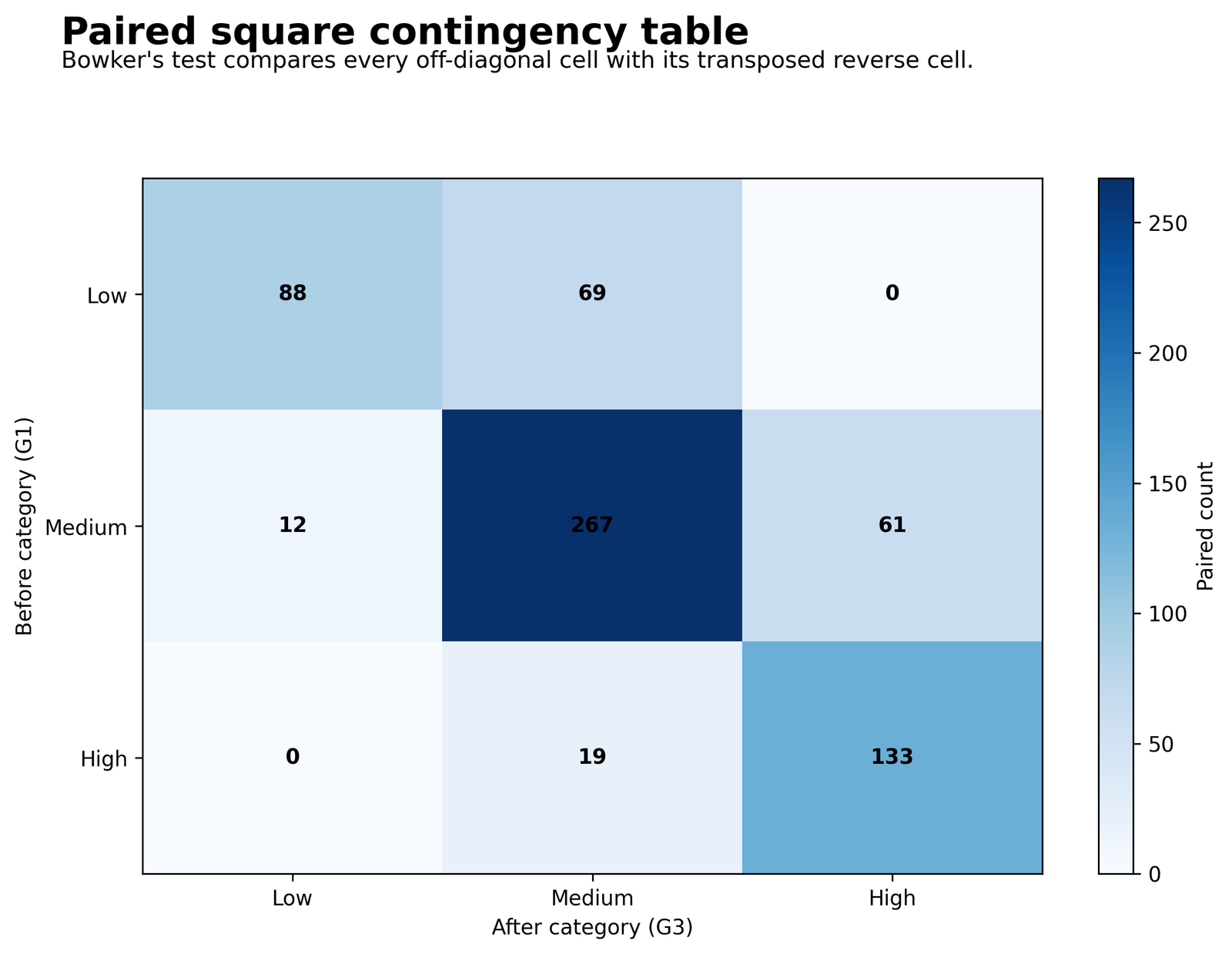
The darkest cell is Medium→Medium with 267 students. Low→Medium and Medium→High are much larger than their reverse cells, whereas the Low↔High pair contains no transitions in either direction.
Diagonal: 88 Low→Low, 267 Medium→Medium, 133 High→High. Discordant: 69 Low→Medium, 12 Medium→Low, 61 Medium→High, 19 High→Medium.
The heatmap makes both stability and directional disagreement visible. The diagonal explains the 75.19% agreement rate; the asymmetric off-diagonal pairs generate the Bowker statistic.
Bowker's Test is calculated from reverse off-diagonal pairs, not from the largest diagonal cell or the overall table colour intensity.
Python Chart 2: Bowker's Test — Directional Asymmetry HeatmapPython
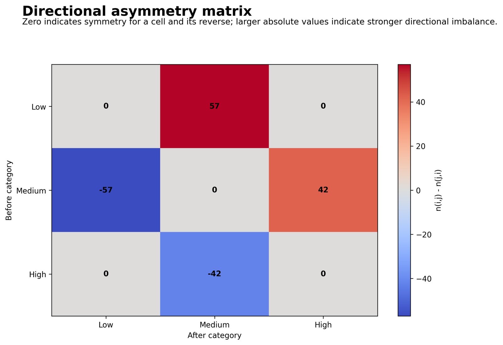
The Low→Medium cell has +57 and its reverse has −57. The Medium→High cell has +42 and its reverse has −42. Low↔High is exactly zero in both directions.
Low versus Medium: ±57. Medium versus High: ±42. Low versus High: 0.
Positive upper-triangle values indicate more upward than downward movement. Both informative category pairs favour the higher grade band at G3.
The signed matrix supplies the substantive direction that the global chi-square statistic does not contain.
Python Chart 3: Bowker's Test — Pairwise Contributions to Bowker's StatisticPython
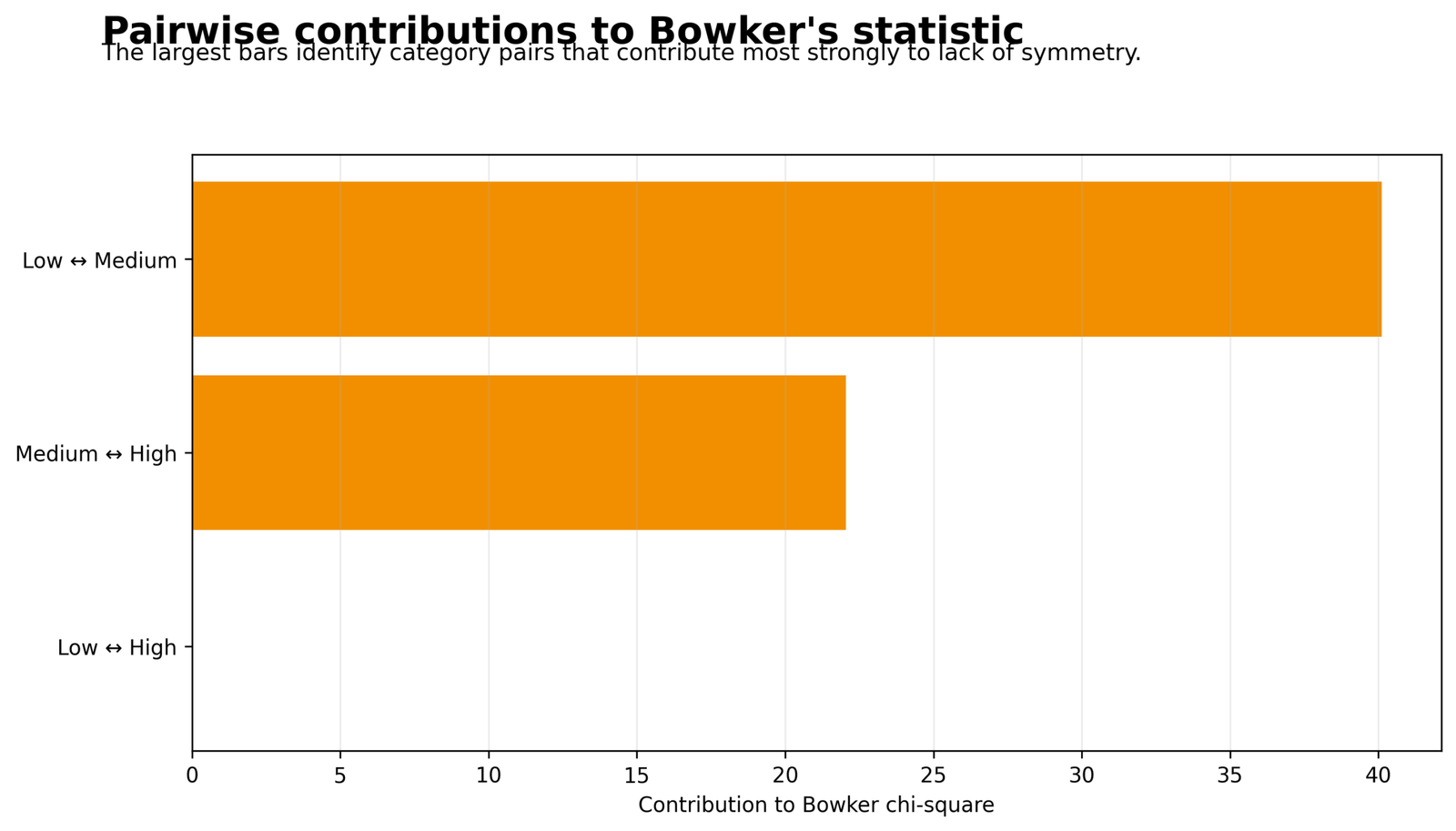
The Low↔Medium bar is the largest. Medium↔High is smaller but still substantial. Low↔High contributes nothing because its discordant total is zero.
Low↔Medium: 40.111111 (64.53%). Medium↔High: 22.050000 (35.47%).
The global statistic of 62.161111 is concentrated in two adjacent-band transitions. Most evidence comes from the movement between Low and Medium.
Contribution analysis identifies the sources of rejection and guides multiplicity-adjusted pairwise McNemar follow-ups.
Python Chart 4: Bowker's Test — Before and After Marginal DistributionsPython
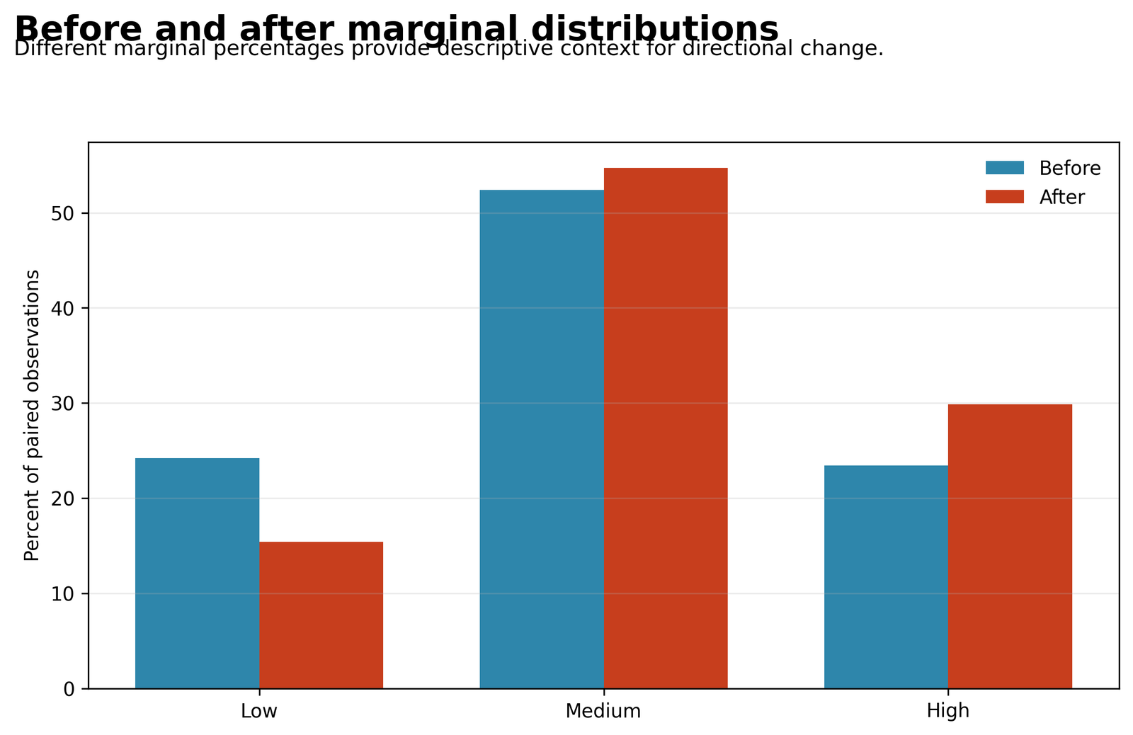
The Low percentage falls sharply, Medium rises modestly, and High rises clearly. The after distribution is shifted toward higher grade bands.
Low: 24.2% to 15.4%. Medium: 52.4% to 54.7%. High: 23.4% to 29.9%.
The marginal changes are −57 Low, +15 Medium, and +42 High. They are consistent with the upward directional transitions.
Marginal distributions provide descriptive context, but Bowker's Test evaluates the stronger condition of cell-by-cell reverse symmetry.
Python Chart 5: Bowker's Test — Opposing Directional Transition CountsPython
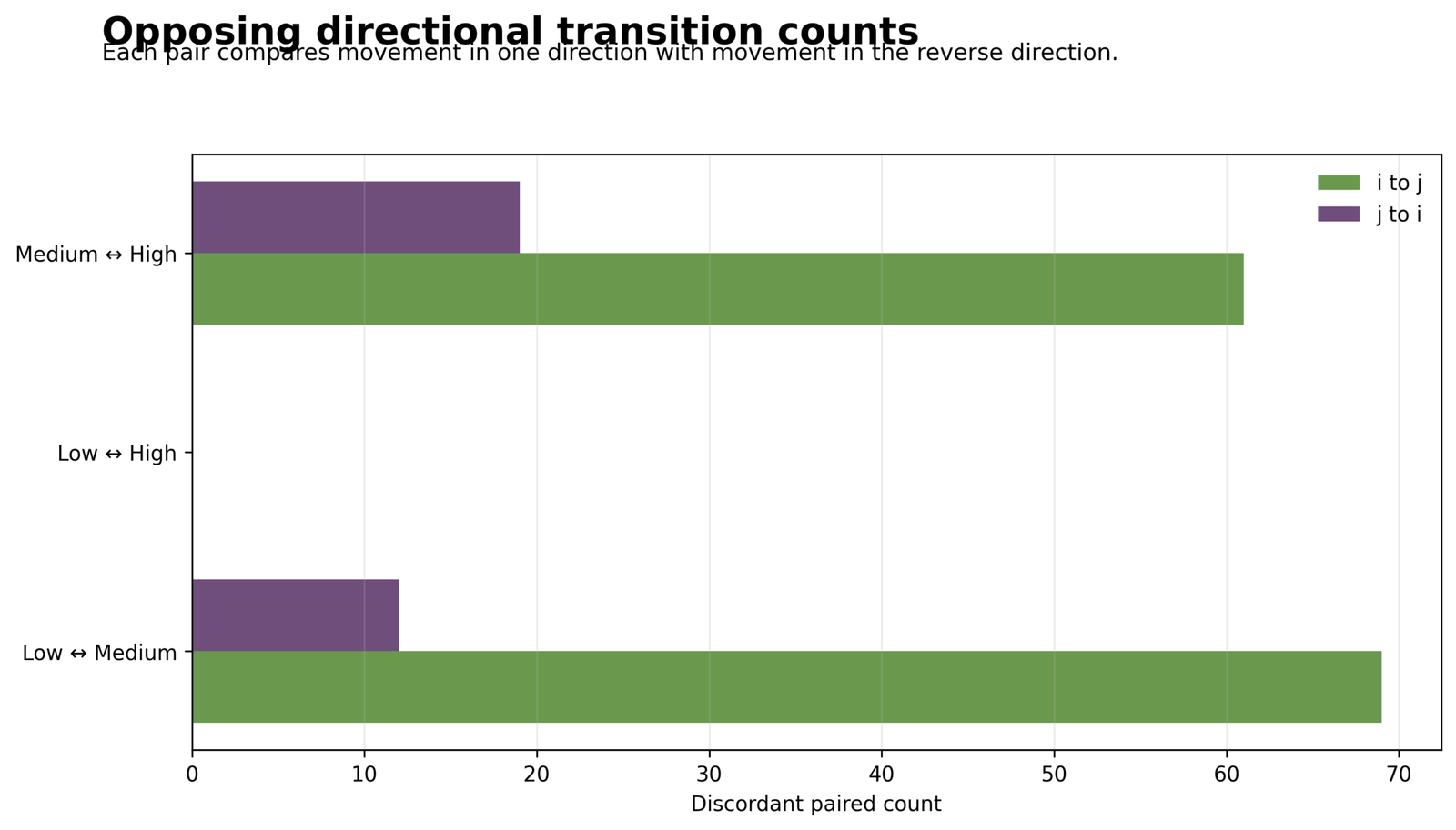
Low→Medium has 69 transitions compared with 12 Medium→Low. Medium→High has 61 compared with 19 High→Medium. Low↔High has no transitions.
Low↔Medium ratio: 69/12 = 5.75. Medium↔High ratio: 61/19 = 3.21.
The direction bars show that rejection is not caused by one isolated category pair. Both informative adjacent-band comparisons favour upward movement.
The chart converts the abstract symmetry hypothesis into directly interpretable paired transition counts.
Python Chart 6: Bowker's Test — Row-Normalized Transition Percentage HeatmapPython
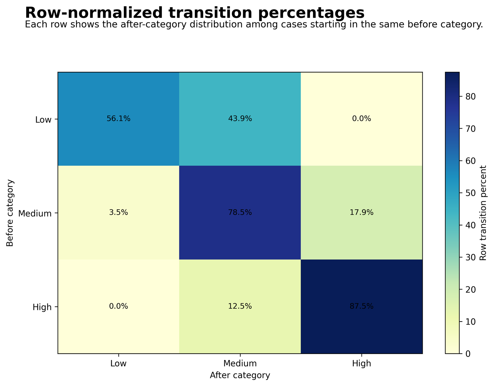
Low students were split between staying Low and moving to Medium. Most Medium students stayed Medium, while 17.9% moved to High. High students were most stable, with 87.5% remaining High.
Low row: 56.1%, 43.9%, 0.0%. Medium row: 3.5%, 78.5%, 17.9%. High row: 0.0%, 12.5%, 87.5%.
Row percentages answer conditional transition questions. They are easier to interpret than raw counts when row totals differ.
The percentage heatmap highlights stability and movement patterns, while the Bowker statistic formally evaluates reverse-count balance.
Python Chart 7: Bowker's Test — Cumulative Contribution to the Test StatisticPython
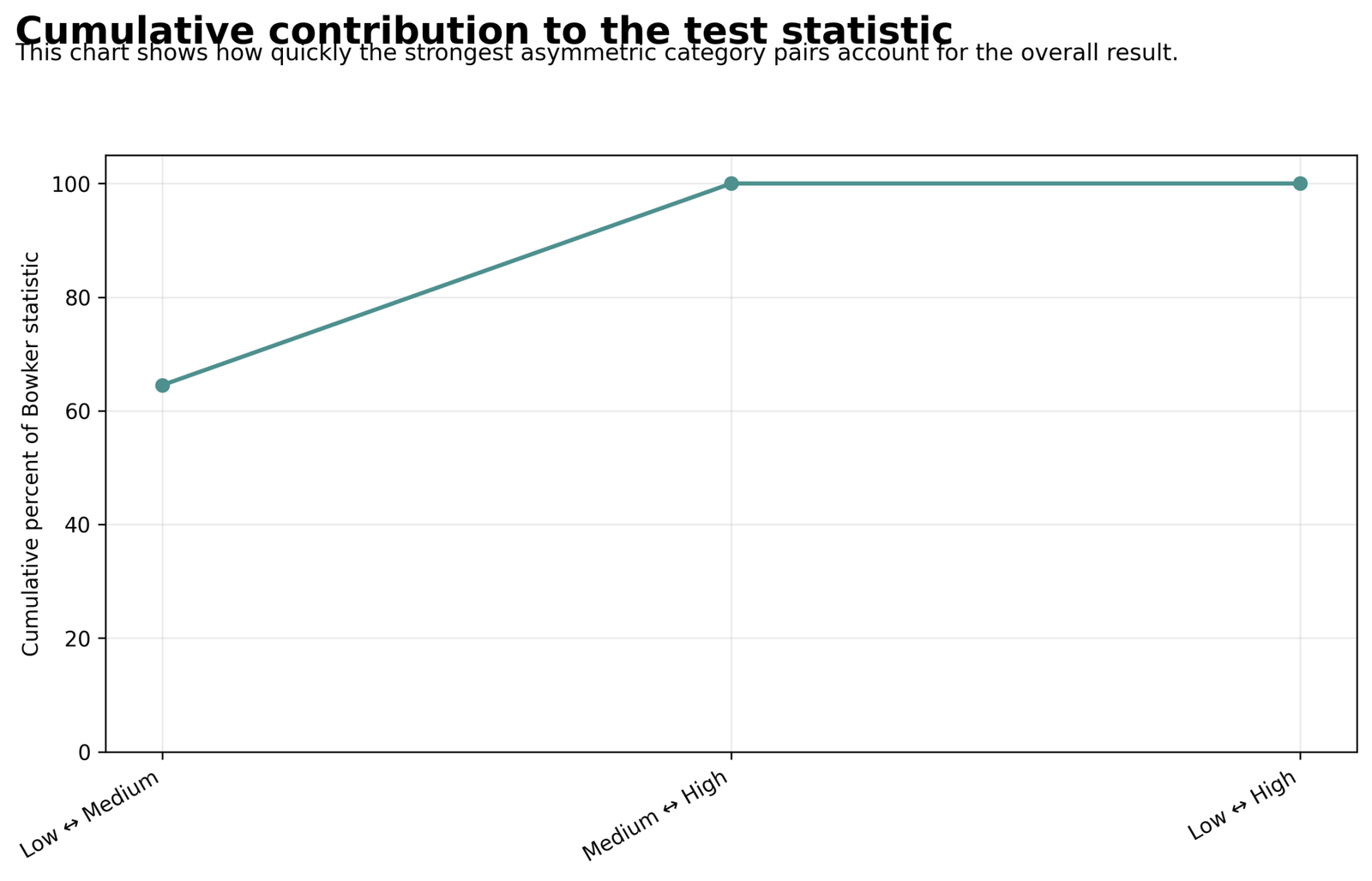
The first pair accounts for approximately 64.53% of the statistic. Adding Medium↔High reaches 100%. The final zero-information pair leaves the cumulative value unchanged.
After Low↔Medium: 64.53%. After Medium↔High: 100.00%.
The global rejection is completely explained by the two adjacent-band pairs. The Low↔High pair adds neither statistical information nor degrees of freedom in the effective-df workflow.
The chart supports a focused post-hoc explanation without hiding the global nature of the Bowker test.
Seven R Bowker Test Charts with Paired Explanations
The R charts are displayed separately from the Python charts, even though the supplied public URLs point to the same rendered image files. The first six R charts appear in three paired rows with a dedicated explanation box under each figure; the cumulative-contribution chart appears in a final full-width row.
R Chart 1: Paired Square Contingency Heatmap
The darkest cell is Medium→Medium with 267 students. Low→Medium and Medium→High are much larger than their reverse cells, whereas the Low↔High pair contains no transitions in either direction. The heatmap makes both stability and directional disagreement visible. The diagonal explains the 75.19% agreement rate; the asymmetric off-diagonal pairs generate the Bowker statistic.
R Chart 2: Directional Asymmetry Heatmap
The Low→Medium cell has +57 and its reverse has −57. The Medium→High cell has +42 and its reverse has −42. Low↔High is exactly zero in both directions. Positive upper-triangle values indicate more upward than downward movement. Both informative category pairs favour the higher grade band at G3.
R Chart 3: Pairwise Contributions to Bowker's Statistic
The Low↔Medium bar is the largest. Medium↔High is smaller but still substantial. Low↔High contributes nothing because its discordant total is zero. The global statistic of 62.161111 is concentrated in two adjacent-band transitions. Most evidence comes from the movement between Low and Medium.
R Chart 4: Before and After Marginal Distributions
The Low percentage falls sharply, Medium rises modestly, and High rises clearly. The after distribution is shifted toward higher grade bands. The marginal changes are −57 Low, +15 Medium, and +42 High. They are consistent with the upward directional transitions.
R Chart 5: Opposing Directional Transition Counts
Low→Medium has 69 transitions compared with 12 Medium→Low. Medium→High has 61 compared with 19 High→Medium. Low↔High has no transitions. The direction bars show that rejection is not caused by one isolated category pair. Both informative adjacent-band comparisons favour upward movement.
R Chart 6: Row-Normalized Transition Percentage Heatmap
Low students were split between staying Low and moving to Medium. Most Medium students stayed Medium, while 17.9% moved to High. High students were most stable, with 87.5% remaining High. Row percentages answer conditional transition questions. They are easier to interpret than raw counts when row totals differ.
R Chart 7: Cumulative Contribution to the Test Statistic
The first pair accounts for approximately 64.53% of the statistic. Adding Medium↔High reaches 100%. The final zero-information pair leaves the cumulative value unchanged. The global rejection is completely explained by the two adjacent-band pairs. The Low↔High pair adds neither statistical information nor degrees of freedom in the effective-df workflow.
Bowker Test Assumptions, Diagnostics and Limitations
Required Conditions
- The same units are measured twice.
- Both measurements use identical categories.
- The table is square.
- Pairs are independent of other pairs.
- Each unit contributes to one table cell.
- Categories are mutually exclusive.
Reporting Checks
- State row and column direction.
- Show the complete square table.
- Report zero-discordance pairs.
- Name the df convention.
- Explain influential category pairs.
- Separate symmetry from agreement.
Paired observations
G1 and G3 must belong to the same student. If the two measurements come from different students, Bowker's Test is not valid because the square table no longer represents within-unit transitions.
Independence between pairs
One student's paired transition should be independent of another student's transition. Students may be clustered within schools or classrooms, so population-level inference can require methods that account for cluster dependence. The exact pairing within each student does not automatically remove dependence between students.
Identical category definitions
The Low, Medium, and High cutpoints must be applied consistently to G1 and G3. If different thresholds are used, the table may still be square in appearance but the reverse-cell comparisons no longer have a coherent interpretation.
Square-table requirement
Every row category needs the same named column category. A rectangular table cannot be symmetric around a main diagonal and requires a different procedure.
Sparse discordant pairs
The Bowker statistic uses a chi-square approximation. Very small reverse-pair totals can make the approximation unreliable. Exact conditional or permutation approaches may be preferred for sparse tables. In the current table, the two informative pair totals are 81 and 80, which are adequate.
Zero discordant pair
The Low↔High pair has 0 and 0. It contains no evidence for or against symmetry. The published analysis excludes the pair from effective df, while some general software retains the nominal maximum df. This choice should be reported because it changes the exact p-value, although not the conclusion here.
Ordinal categories and distance
Bowker's formula treats every category pair as a distinct nominal comparison. A one-band movement and a two-band movement do not receive distance weights. If distance is substantively important, supplement Bowker with weighted agreement measures or an ordinal repeated-outcome model.
Agreement is a separate concept
The diagonal agreement rate is 75.19%, unweighted κ is 0.591, and weighted kappas are higher because adjacent-category disagreements receive partial credit. None of these values changes the Bowker p-value because the symmetry statistic excludes diagonal counts.
Marginal homogeneity is a separate null
Stuart-Maxwell tests whether the before and after marginal proportions are equal. Bowker tests every reverse-cell equality. The two tests can disagree because complete symmetry is stronger than equal margins.
Dichotomizing or collapsing categories
Collapsing Low, Medium, and High into two categories would permit ordinary McNemar analysis but discard transition detail. Category reduction should be based on the research question rather than on obtaining a preferred p-value.
Missing paired observations
A complete Bowker table requires both measurements. Pairwise deletion can change the analysed population if missingness is related to grade or transition direction. Report the number of complete pairs and the missing-data rule.
Causal interpretation
The significant upward asymmetry does not prove that time or a particular intervention caused improvement. The data describe paired grade transitions; causal explanation requires a suitable design and control of alternative influences.
Bowker's Test in Python, R, SPSS and Excel
Bowker Test in Python
Python can calculate Bowker symmetry through a manual reverse-pair loop or a square-table function. A manual calculation is useful when zero-discordance pairs require an explicit effective-df rule.
- Recategorize G1 and G3 using identical bands.
- Create a square crosstab in the same category order.
- Loop through i < j reverse pairs.
- Skip pairs with nij + nji = 0 when using effective df.
- Use the upper-tail chi-square probability.
Expected result: χ² = 62.161111, df = 2, p = 3.17604193e-14.
Bowker Test in R
Base R's mcnemar.test() extends to larger square tables and tests symmetry. A manual contribution table can preserve the same zero-pair rule and provide pair-level diagnostics.
- Create factors with levels Low, Medium, High.
- Build
table(before, after). - Run
mcnemar.test()for the general square-table result. - Calculate reverse-pair contributions explicitly.
- Use
binom.test()for exact pairwise McNemar follow-ups.
The downloadable R report gives χ² = 62.161111, effective df = 2, and p = 3.17604193e-14.
Bowker Test in SPSS
SPSS can prepare the paired categories, produce the square crosstab, row percentages, marginal frequencies, and transition graph. The Bowker statistic can be calculated with matrix logic or embedded Python when the standard menus do not provide the required multi-category symmetry output.
- Create identical numeric grade-band variables for G1 and G3.
- Use CROSSTABS to verify the 3 × 3 table.
- Request row, column, and total percentages.
- Use embedded Python for the reverse-pair contribution calculation.
- Export the crosstab and supporting output with the exact table direction stated.
Bowker Test in Excel
Excel can reproduce the entire test transparently. The worked workbook should contain the paired square table, reverse-pair calculations, effective degrees of freedom, p-value, marginal distributions, transition percentages, post-hoc tests, and reporting output.
- Enter the 3 × 3 observed table.
- Reference each upper-triangle cell and its transpose.
- Calculate squared difference divided by pair total.
- Count nonzero discordant pair totals for effective df.
- Use
CHISQ.DIST.RTfor the p-value.
Cross-Software Values That Must Match
| Element | Verified value | Reporting role |
|---|---|---|
| Complete paired observations | 649 | Analysis sample size |
| Square table | [[88,69,0],[12,267,61],[0,19,133]] | Primary data input |
| Bowker statistic | 62.161111111 | Global symmetry statistic |
| Effective df | 2 | Informative reverse pairs |
| P-value | 3.17604193e-14 | Reject symmetry |
| Agreement count | 488 | Descriptive stability |
| Discordant count | 161 | Total changed cases |
| Directional asymmetry index | 0.614906832 | Net imbalance among changes |
Expandable Bowker Test Code
Python: manual Bowker test with effective degrees of freedom
import numpy as np
from scipy.stats import chi2

table = np.array([
    [88, 69, 0],
    [12, 267, 61],
    [0, 19, 133],
], dtype=float)

statistic = 0.0
effective_df = 0
pair_details = []

k = table.shape[0]

for i in range(k):
    for j in range(i + 1, k):
        forward = table[i, j]
        reverse = table[j, i]
        discordant_total = forward + reverse

        if discordant_total == 0:
            contribution = 0.0
        else:
            contribution = (
                (forward - reverse) ** 2
                / discordant_total
            )
            statistic += contribution
            effective_df += 1

        pair_details.append({
            "i": i,
            "j": j,
            "forward": forward,
            "reverse": reverse,
            "contribution": contribution,
        })

p_value = chi2.sf(statistic, effective_df)

print("Bowker chi-square:", statistic)
print("Effective df:", effective_df)
print("P-value:", p_value)
print(pair_details)
Python: build grade bands from the source dataset
import pandas as pd

df = pd.read_csv("dataset.csv")

labels = ["Low", "Medium", "High"]
bins = [-0.5, 9.5, 13.5, float("inf")]

df["before_band"] = pd.cut(
    df["G1"],
    bins=bins,
    labels=labels,
    ordered=True,
)

df["after_band"] = pd.cut(
    df["G3"],
    bins=bins,
    labels=labels,
    ordered=True,
)

paired_table = pd.crosstab(
    df["before_band"],
    df["after_band"],
    dropna=False,
).reindex(index=labels, columns=labels, fill_value=0)

print(paired_table)
Python: exact pairwise McNemar follow-ups
from scipy.stats import binomtest

pairs = [
    ("Low", "Medium", 69, 12),
    ("Low", "High", 0, 0),
    ("Medium", "High", 61, 19),
]

for category_i, category_j, i_to_j, j_to_i in pairs:
    discordant_total = i_to_j + j_to_i

    if discordant_total == 0:
        p_value = None
    else:
        p_value = binomtest(
            min(i_to_j, j_to_i),
            n=discordant_total,
            p=0.5,
            alternative="two-sided",
        ).pvalue

    print(
        category_i,
        category_j,
        i_to_j,
        j_to_i,
        p_value,
    )
R: Bowker symmetry and pair contribution table
paired_table <- matrix(
  c(
    88, 69, 0,
    12, 267, 61,
    0, 19, 133
  ),
  nrow = 3,
  byrow = TRUE,
  dimnames = list(
    Before = c("Low", "Medium", "High"),
    After = c("Low", "Medium", "High")
  )
)

# General square-table symmetry procedure.
print(mcnemar.test(paired_table))

# Manual effective-df version.
statistic <- 0
effective_df <- 0
details <- list()

for (i in 1:(nrow(paired_table) - 1)) {
  for (j in (i + 1):ncol(paired_table)) {
    forward <- paired_table[i, j]
    reverse <- paired_table[j, i]
    pair_total <- forward + reverse

    if (pair_total == 0) {
      contribution <- 0
    } else {
      contribution <-
        (forward - reverse)^2 / pair_total
      statistic <- statistic + contribution
      effective_df <- effective_df + 1
    }

    details[[length(details) + 1]] <- c(
      i = i,
      j = j,
      forward = forward,
      reverse = reverse,
      contribution = contribution
    )
  }
}

p_value <- pchisq(
  statistic,
  df = effective_df,
  lower.tail = FALSE
)

print(statistic)
print(effective_df)
print(p_value)
print(details)
Base R may retain the nominal degrees of freedom in its general result. Use the manual calculation when reproducing the effective-df convention used in the supplied reports.
SPSS: create paired grade bands and verify the square table
* Create identical grade bands for G1 and G3.
RECODE G1
  (Lowest THRU 9=1)
  (10 THRU 13=2)
  (14 THRU Highest=3)
  INTO bowker_before.

RECODE G3
  (Lowest THRU 9=1)
  (10 THRU 13=2)
  (14 THRU Highest=3)
  INTO bowker_after.

VALUE LABELS bowker_before bowker_after
  1 "Low (0-9)"
  2 "Medium (10-13)"
  3 "High (14+)".
EXECUTE.

* Verify the paired square table.
CROSSTABS
  /TABLES=bowker_before BY bowker_after
  /FORMAT=AVALUE TABLES
  /CELLS=COUNT ROW COLUMN TOTAL
  /COUNT ROUND CELL.

* Use embedded Python or matrix logic for the
* reverse-pair Bowker contribution calculation.
Excel: formula layout for Bowker's Test
Assume the 3 x 3 observed table is B5:D7.

Low-Medium contribution:
=(C5-B6)^2/(C5+B6)

Low-High contribution:
=IF(D5+B7=0,0,(D5-B7)^2/(D5+B7))

Medium-High contribution:
=(D6-C7)^2/(D6+C7)

Bowker statistic:
=SUM(contribution_cells)

Effective degrees of freedom:
=COUNTIF(discordant_pair_total_cells,">0")

P-value:
=CHISQ.DIST.RT(
  bowker_statistic_cell,
  effective_df_cell
)

Agreement count:
=SUM(B5,C6,D7)

Discordant count:
=SUM(B5:D7)-agreement_count

Directional asymmetry index:
=(upward_total-downward_total)/discordant_count
Advanced Bowker Test Topics
Nominal versus effective degrees of freedom
For a k × k table, the nominal maximum df is k(k−1)/2. This assumes that every reverse pair can contribute information. When both cells in a reverse pair are zero, the contribution denominator is zero and the pair carries no symmetry information. Some workflows reduce df to the number of informative pair totals; others retain the nominal maximum. Report the convention and software because the p-value can differ.
Why the current df difference does not change the decision
With χ² = 62.161111, effective df = 2 gives p = 3.17604193e-14, while nominal df = 3 gives p = 2.02960250e-13. Both values are far below .001. The degrees-of-freedom issue matters for reproducibility even though it does not alter the substantive conclusion in this dataset.
Exact alternatives for sparse tables
The standard Bowker procedure uses an asymptotic chi-square distribution. When several discordant pair totals are small, an exact conditional test, permutation approach, or Monte Carlo method can provide a more reliable finite-sample reference. Exact methods require a clearly stated definition of tables at least as extreme as the observed table.
Pairwise exact McNemar tests
Each reverse category pair forms a paired 2 × 2 discordance question. Conditional on the pair total, symmetry implies a .50 probability in either direction. Exact binomial tests therefore provide natural pairwise follow-ups. Multiplicity adjustment is required when the pair-level conclusions are treated as confirmatory.
Bowker symmetry versus marginal homogeneity
Complete symmetry requires pij = pji for every off-diagonal pair. Marginal homogeneity requires only that the before and after category proportions match. Symmetry implies marginal homogeneity, but the converse is not generally true. A table can have equal margins while opposing asymmetries cancel.
Why Bowker and Stuart-Maxwell are identical here
The Low↔High reverse pair contains no discordant observations, leaving two adjacent-category directions. In this specific three-category structure, the effective-df Bowker and Stuart-Maxwell calculations produce the same statistic and p-value. This numerical equality should not be generalized to other tables.
Ordered-category directional summaries
Bowker's chi-square treats categories nominally, but ordered labels permit useful summaries. Upward transitions total 130, downward transitions total 31, and the upward/downward ratio is 4.194. These summaries explain direction but do not replace the global test.
Directional asymmetry index
The descriptive index used in the reports is (upward − downward)/(upward + downward). It equals 0.614907. The index ranges from −1 to 1: positive values indicate net upward movement, negative values indicate net downward movement, and zero indicates balanced directional totals. It is not a standardized inferential effect size.
Agreement statistics beside Bowker's Test
Simple agreement is 75.19% and unweighted κ is 0.591. Linear-weighted κ = 0.653 and quadratic-weighted κ = 0.734. Weighted agreement is higher because most discordance occurs between adjacent bands rather than between Low and High.
Cumulative contribution analysis
Sorting reverse pairs by contribution shows that Low↔Medium explains 64.53% of the statistic. Medium↔High supplies the remaining 35.47%. This decomposition is useful for explanation, but the global test remains the primary inferential statement.
Power and sample-size planning
Power depends on the paired table probabilities, number of categories, sample size, and distribution of asymmetry across reverse pairs. Planning should specify a plausible transition matrix rather than only an overall agreement rate. See Statistical Power before designing a new paired categorical study.
Covariate-adjusted alternatives
Bowker's Test is unadjusted. When transition direction may vary by school, sex, prior achievement, or another covariate, consider multinomial models, marginal models, generalized estimating equations, or stratified analyses. A single global square table cannot separate confounding or effect modification.
More than two repeated measurements
Pairwise Bowker tests across many time points increase multiplicity and do not jointly model the repeated trajectory. Longitudinal categorical methods are more appropriate when the research question concerns change across three or more occasions.
Structural zeros versus sampling zeros
A structural zero means a transition is impossible by design; a sampling zero means it was possible but not observed. The Low↔High zeros here may reflect the chosen broad grade bands and observed data rather than impossibility. The distinction matters for model interpretation and degrees-of-freedom decisions.
APA Reporting for Bowker's Test of Symmetry
A complete APA-style report should identify the paired variables, category definitions, sample size, square table, test statistic, degrees of freedom, p-value, decision, influential reverse pairs, and substantive direction. Agreement measures can be added separately but should not be presented as Bowker effect sizes.
Full APA-Style Result for the Worked Example
G1 and G3 grades from 649 students were classified as Low (0–9), Medium (10–13), or High (14+). Bowker's Test of Symmetry indicated that the paired grade-band transition table was not symmetric, χ²(2) = 62.16, p < .001. Low→Medium transitions (69) exceeded Medium→Low transitions (12), and Medium→High transitions (61) exceeded High→Medium transitions (19). Of the 161 students who changed bands, 130 (80.7%) moved upward and 31 (19.3%) moved downward. The simple diagonal agreement rate was 75.19%.
Concise APA-Style Result
Bowker's Test showed asymmetric G1-to-G3 grade-band transitions, χ²(2) = 62.16, p < .001, with 130 upward and 31 downward changes.
APA-Style Methods Sentence
G1 and G3 were recoded into identical Low, Medium, and High grade bands, and Bowker's Test of Symmetry was used to compare each off-diagonal transition count with its reverse transition count.
APA-Style Results Table
| Measure | Complete value | APA presentation |
|---|---|---|
| Complete paired observations | 649 | N = 649 |
| Bowker chi-square | 62.161111111 | χ² = 62.16 |
| Effective df | 2 | df = 2 |
| P-value | 3.17604193e-14 | p < .001 |
| Agreement count | 488 | 488/649 |
| Agreement rate | 0.751926040 | 75.19% |
| Discordant count | 161 | 161 |
| Upward transitions | 130 | 130 (80.7% of changes) |
| Downward transitions | 31 | 31 (19.3% of changes) |
| Directional asymmetry index | 0.614906832 | .615 |
Reusable APA Templates for Bowker's Test
Significant Bowker Test of Symmetry
Before variable and after variable were classified into the same k categories for N paired observations.
Bowker's Test indicated that the paired transition table was asymmetric, χ²(df) = statistic, p = p-value.
The largest directional differences occurred for category pair 1 and category pair 2, with substantive direction.
Report the complete table or enough reverse-pair counts for the result to be understood.
Nonsignificant Bowker Test of Symmetry
A k × k paired table summarized before and after categories for N observations.
Bowker's Test was not statistically significant, χ²(df) = statistic, p = p-value.
The analysis did not provide sufficient evidence that reverse transition probabilities were unequal; it did not prove perfect symmetry or agreement.
Include the transition counts and confidence or descriptive context rather than interpreting nonsignificance as equality.
Pairwise Exact McNemar Follow-Up
For the category i ↔ category j comparison, nij observations moved in one direction and nji moved in the reverse direction.
The exact paired comparison was significant / not significant, adjusted p = p-value.
The imbalance favoured direction, contributing percentage of the global Bowker statistic.
Conduct pairwise tests after the global result and apply the prespecified multiplicity correction.
APA Rounding and Language Rules
| Avoid | Use instead | Reason |
|---|---|---|
| p = .000 | p < .001 | The probability is extremely small, not zero. |
| Grades improved because Bowker was significant. | Observed grade-band transitions were predominantly upward. | The test does not establish causation. |
| Agreement was significant. | The transition table was asymmetric. | Bowker tests symmetry, not agreement. |
| χ²(3) without explaining the zero pair | State the effective or nominal df convention. | Software can handle zero-discordance pairs differently. |
| All categories changed. | Low↔Medium and Medium↔High were asymmetric; Low↔High had no transitions. | The pair-level pattern is specific. |
Common Bowker Test Mistakes and How to Correct Them
| Common mistake | Why it is wrong | Correct approach |
|---|---|---|
| Using independent groups | Bowker requires matched observations. | Use a test for independent categorical samples. |
| Using different category definitions before and after | Reverse cells no longer represent the same categories. | Apply identical labels and cutpoints. |
| Analysing a rectangular table | A rectangular table has no complete diagonal symmetry. | Use a method for rectangular paired data. |
| Including diagonal counts in the formula | Diagonal cells do not measure directional imbalance. | Use only i<j off-diagonal pairs. |
| Dividing by zero for an empty pair | A 0/0 contribution is undefined. | Assign zero contribution and disclose the df rule. |
| Calling the result an agreement test | Symmetry and agreement are different hypotheses. | Report kappa separately when needed. |
| Reporting only the global p-value | The direction and contributing pairs remain hidden. | Show signed pair differences and contributions. |
| Running unadjusted pairwise tests after significance | Multiple comparisons inflate false positives. | Use Holm or Bonferroni correction. |
| Using ordinary McNemar on a 3 × 3 table | One binary comparison cannot test complete symmetry. | Use Bowker globally, then pairwise McNemar follow-ups. |
| Interpreting p<.001 as a large effect | Significance depends on sample size and imbalance. | Report transition counts and directional summaries. |
| Ignoring category order | Direction cannot be interpreted substantively. | State whether movement is upward, downward, or nominal. |
| Claiming causal improvement | The paired table alone does not identify a cause. | Use descriptive change language. |
Bowker Test Reports and Worked Excel Download
R Bowker Test ReportR symmetry analysis, exact pairwise results, directional summaries, and seven chart pages.
SPSS Bowker Test OutputPaired category frequencies, 3 × 3 crosstab, percentages, and supporting SPSS output.
Worked Bowker Test Excel WorkbookEditable paired table, contribution formulas, degrees of freedom, p-value, post-hoc calculations, and reporting.
Frequently Asked Questions About Bowker's Test of Symmetry
The questions below address the Bowker test formula, assumptions, degrees of freedom, calculator logic, McNemar-Bowker terminology, software, agreement, marginal homogeneity, post-hoc tests, and APA reporting without repeating the complete worked sections above.
What is Bowker's Test of Symmetry?
It is a chi-square test of whether every off-diagonal transition count in a paired square categorical table equals its reverse transition count.
What is the McNemar-Bowker test?
It is another name for Bowker's multi-category extension of McNemar's paired binary symmetry test.
What is the null hypothesis?
For every pair of categories i and j, the probability of i-to-j movement equals the probability of j-to-i movement.
What data does Bowker's Test require?
The same units must be measured twice using the same categorical scale, producing a square contingency table.
Can Bowker's Test be used for independent samples?
No. It is designed for paired or matched observations.
Can it be used with two categories?
Yes mathematically, but it reduces to ordinary McNemar's test.
Can it be used with three categories?
Yes. The worked example uses Low, Medium, and High grade bands.
What is the Bowker formula?
Sum (n_ij minus n_ji) squared divided by (n_ij plus n_ji) over all unique off-diagonal pairs.
What is the test statistic in this example?
The Bowker chi-square statistic is 62.161111.
What are the degrees of freedom?
The supplied workflow uses effective df = 2 because the Low↔High discordant pair total is zero.
Why might another program report df = 3?
Some programs retain the nominal k(k-1)/2 degrees of freedom even when a reverse pair has zero total.
What is the p-value?
Using effective df = 2, the p-value is approximately 3.17604193e-14.
What is the conclusion?
Reject symmetry; the observed paired transitions are strongly directional.
How many students stayed in the same category?
488 of 649, or 75.19%, remained on the diagonal.
How many students changed category?
161 students changed grade band.
How many transitions were upward?
There were 130 upward transitions.
How many transitions were downward?
There were 31 downward transitions.
What is the directional asymmetry index?
It is 0.614907, indicating strong net upward movement among changed cases.
Which pair contributed most?
Low↔Medium contributed 40.111111, or 64.53% of the statistic.
What was the Medium↔High contribution?
It contributed 22.050000, or 35.47%.
Why did Low↔High contribute zero?
No students moved directly in either direction, so the discordant pair total was zero.
What are the pairwise exact p-values?
Low↔Medium p = 7.03300083e-11; Medium↔High p = 2.73186992e-06.
Does Bowker's Test measure agreement?
No. Agreement can be described with diagonal agreement or kappa, while Bowker tests directional symmetry.
What is Cohen's kappa here?
The unweighted kappa is 0.591.
What is linear-weighted kappa?
The linear-weighted kappa is 0.653.
What is quadratic-weighted kappa?
The quadratic-weighted kappa is 0.734.
What is the difference between Bowker and Stuart-Maxwell?
Bowker tests complete reverse-cell symmetry; Stuart-Maxwell tests equality of the marginal distributions.
Why are Bowker and Stuart-Maxwell numerically equal here?
The particular three-category table has no Low↔High discordance, causing the two effective-df calculations to coincide.
Does Bowker require expected counts above 5?
The standard test uses a chi-square approximation, but the relevant quantities are reverse-pair discordant totals rather than ordinary independence expected counts.
What should be done with sparse pairs?
Use an exact or permutation symmetry procedure and report the method.
How do I run Bowker's Test in Python?
Build the square table and sum reverse-pair contributions manually or use a square-table symmetry function, while checking its df convention.
How do I run Bowker's Test in R?
Use mcnemar.test on the square table or calculate the pair contributions manually for the desired df convention.
How do I run Bowker's Test in SPSS?
Create identical categorical before and after variables, verify the crosstab, and calculate the statistic with matrix logic or embedded Python.
Can Excel calculate Bowker's Test?
Yes. Excel can calculate every reverse-pair contribution, effective df, chi-square p-value, transition percentages, and pairwise exact follow-ups.
How should the result be reported in APA style?
Report N, category definitions, the square-table direction, chi-square, df, p-value, influential reverse pairs, and substantive transition direction.
What is the main conclusion from the worked example?
Grade-band transitions from G1 to G3 were strongly asymmetric and predominantly upward.
Bowker's Test of Symmetry Conclusion
Bowker's Test of Symmetry is the appropriate global procedure when the same observational units are classified twice using the same three or more categories and the research question concerns directional balance between reverse transitions.
In the worked analysis, 649 students were classified into Low, Medium, and High grade bands at G1 and G3. The paired table produced χ² = 62.161111, effective df = 2, and p = 3.17604193e-14. The null hypothesis of symmetry was rejected.
The result was driven by 69 Low→Medium versus 12 Medium→Low transitions and 61 Medium→High versus 19 High→Medium transitions. Overall, 130 students moved upward and 31 moved downward among the 161 changed cases.

