
Zero Inflated Poisson Regression: Formula, Results, Interpretation and Diagnostics
Learn how Zero Inflated Poisson Regression separates a structural-zero process from a Poisson count process, then interpret the verified 649-case results, rate ratios, zero odds, predictions, diagnostics and software output.
244 observed zeros
ZIP AIC 3388.48
Python, R, SPSS and Excel
Zero Inflated Poisson Regression Model Overview
Zero Inflated Poisson Regression is a two-part count model for a nonnegative integer outcome that contains more zeros than a conventional Poisson regression can plausibly represent. It answers two related questions at the same time: which variables are associated with the expected count among observations that can generate counts, and which variables are associated with membership in an additional zero-generating state?
The method is most useful when the outcome is a count, the observation period or exposure is comparable across cases, zeros are unusually common, and there is a defensible reason to believe that some zeros arise from a different mechanism than positive counts. Examples include service use when some people are not eligible to use the service, equipment failures when some units are not exposed to risk, purchases when some customers are not in the market, or event counts when some cases are effectively immune during the study window.
A standard Poisson regression uses one log-linked equation and assumes that every zero is a sampling zero from the same count distribution that generates one, two, three and larger counts. Zero Inflated Poisson Regression adds a logit equation for an unobserved structural-zero state. The final probability distribution is therefore a mixture: one component always produces zero, while the other produces counts according to a Poisson distribution and can itself produce zero by chance.
The inflation equation converts predictors into the probability π that a case belongs to the always-zero state.
The count equation converts predictors into λ, the expected count for cases in the count-generating state.
The unconditional mean is (1 − π)λ, and the total probability of zero includes both structural and Poisson zeros.
Coefficients from the two equations have different meanings. Exponentiating a count-component coefficient gives an incidence rate ratio, or IRR, describing the multiplicative change in λ for a one-unit predictor increase while other count predictors remain fixed. Exponentiating an inflation coefficient gives an odds ratio for structural-zero membership. An odds ratio above one increases the odds of belonging to the additional zero state; it does not increase the expected positive count.
Zero Inflated Poisson Regression differs from several related methods. A negative binomial model addresses overdispersion with one count process but does not create a separate structural-zero state. A zero-inflated negative binomial model combines both ideas and is often preferable when extra zeros and positive-count overdispersion occur together. A hurdle model also has two equations, but every zero comes from the first equation and the positive-count distribution is truncated at zero. Ordinary logistic regression discards the size of positive counts, while ordinary linear regression can produce impossible negative predictions and does not model count probabilities.
Supported variables
- A nonnegative integer outcome with meaningful zeros.
- Continuous, binary, ordinal or dummy-coded categorical predictors.
- Different predictor sets in the count and inflation equations.
- An exposure offset when cases are observed for unequal amounts of time.
Core assumptions
- Independent observations unless clustering is modelled explicitly.
- A correctly specified log link for the count mean and logit link for inflation.
- Conditional Poisson variance within the count-generating state.
- A substantively defensible and statistically identifiable extra-zero process.
The main advantage of Zero Inflated Poisson Regression is its ability to represent excess zeros without discarding positive-count information. It also provides separate scientific interpretations for count intensity and zero-state membership. Its limitations are equally important: latent class membership is never observed directly, the model can be difficult to identify when the two equations use weak predictors, and zero inflation does not automatically solve overdispersion among positive counts.
The worked example uses 649 student records and models absences. There are 244 zeros, representing 37.5963% of the sample. The count equation uses G1, G2, studytime, failures, age and health; the inflation equation uses failures, age and health. The observed mean is 3.6595, the variance is 21.5366, and the variance-to-mean ratio is 5.8852. Those values establish both an excess-zero question and a broader dispersion question that must remain visible throughout the analysis.
Quick Answer
Why the ZIP model is preferred
- ZIP log likelihood is −1683.2399, compared with −2330.3782 for standard Poisson.
- ZIP AIC is 3388.4798, compared with 4674.7564 for Poisson.
- The Vuong comparison gives z = 12.0433 and p = 2.10 × 10⁻³³.
- The model predicts 243.8578 zeros against 244 observed.
Why the model still needs caution
- The raw variance is 5.8852 times the mean.
- Large positive counts remain underpredicted.
- ZIP RMSE is 4.5596, slightly above Poisson RMSE of 4.5276.
- None of the three inflation slopes is individually significant at α = .05.
Bottom line: Zero Inflated Poisson Regression provides a far better probability model for the large mass at zero, but it does not fully resolve positive-count overdispersion or produce sharper case-level zero discrimination. A zero-inflated negative binomial sensitivity model is therefore a logical next comparison.
Table of Contents
- Model Overview
- Quick Answer
- Why Zero Inflated Poisson Regression Is Needed
- How Zero Inflated Poisson Regression Works
- Variables and Data Dictionary
- Verified Model Results
- Python Charts and Explanations
- R Charts and Explanations
- Coefficient Interpretation
- Predictions and Marginal Meaning
- Assumptions and Diagnostics
- Python, R, SPSS and Excel
- Expandable Code
- Advanced Topics
- APA-Style Reporting
- Publication Checklist
- Downloads
- Related Guides
- Frequently Asked Questions
- Conclusion
Why This Analysis Needs Zero Inflated Poisson Regression
The outcome is a count of absences, so its values are nonnegative integers rather than unrestricted continuous measurements. A Gaussian linear model would ignore the discrete probability structure and could produce negative fitted counts. A standard Poisson regression respects the count scale, but it assigns all observations to one count-generating process and expects its conditional variance to equal its conditional mean.
The decisive signal is not merely that zeros are common. Many legitimate Poisson datasets contain many zeros when their expected counts are small. The stronger evidence is that the fitted standard Poisson model predicts only 24.6591 zeros while the data contain 244. That difference shows that the single-process Poisson specification allocates far too little probability mass to zero.
Zero Inflated Poisson Regression addresses this mismatch by adding a latent state that produces only zeros. For this analysis, failures, age and health enter the inflation equation, while G1, G2, studytime, failures, age and health enter the count equation. The two sets need not be identical because the factors associated with being effectively in a zero state can differ from the factors associated with the number of absences among count-generating cases.
A hurdle model would also create two equations, but it would treat every observed zero as arising from the zero equation and every positive count as arising from a zero-truncated count model. Zero Inflated Poisson Regression is more appropriate when some zeros may still be ordinary Poisson outcomes. A zero-inflated negative binomial model may ultimately be more flexible because the present data show substantial variation beyond the zero mass.
How Zero Inflated Poisson Regression Works
Two Linear Predictors and Two Link Functions
Zero Inflated Poisson Regression begins with two separate linear predictors. The count equation uses a log link so that the Poisson mean is always positive. The inflation equation uses a logit link so that the structural-zero probability always lies between zero and one.
Inflation component: logit(πi) = z′iγ, therefore πi = exp(z′iγ) / [1 + exp(z′iγ)]
Here, λi is the expected Poisson count for case i if that case belongs to the count-generating state. The quantity πi is the probability that the case belongs to the structural-zero state. A case with a high π can still have a large count-state mean λ; the unconditional expected count depends on both quantities.
The Mixture Probability for Zero and Positive Counts
P(Yi = y) = (1 − πi)exp(−λi)λiy/y!, for y = 1, 2, 3, …
The zero formula contains two routes. The first term, π, is the probability of an automatic structural zero. The second term is the probability of entering the count state and then drawing zero from the Poisson distribution. For positive outcomes, the case must first be in the count state, which explains the multiplier 1 − π.
This distinction prevents a common interpretation error. The model does not label observed zeros as structural or sampling zeros. It estimates probabilities for unobserved membership. Posterior classification can be calculated, but it remains probabilistic and should not be presented as known truth.
Expected Count and Total Zero Probability
The count-state mean λ is not the final expected outcome. Multiplying by the probability of being in the count state produces the unconditional expected count. In the supplied prediction file, the count-state mean and the ZIP predicted mean are stored separately. The unconditional mean is the appropriate fitted value for observed-versus-predicted count plots and point-error calculations.
The total probability of zero is also different from π. It is always at least as large as π because a case in the count state can still generate zero. A chart labelled “predicted zero probability” should therefore be checked carefully to determine whether it displays π alone or the complete mixture probability.
Interpreting Count Coefficients as Incidence Rate Ratios
For a one-unit increase in predictor xj, the count-state mean λ is multiplied by exp(βj) while other count predictors are held constant. An IRR of 1.10 indicates a 10% higher expected count in the Poisson state; an IRR of 0.90 indicates a 10% lower expected count. This is a conditional count-state effect, not automatically the same as the percentage change in the unconditional mean.
In the worked model, age has an IRR of 1.1044, implying approximately 10.44% higher expected absences in the count state for each one-year increase, conditional on the other count predictors. Studytime has an IRR of 0.8976, implying approximately 10.24% lower expected count per one-unit increase in the studytime score.
Interpreting Inflation Coefficients as Structural-Zero Odds Ratios
An inflation odds ratio describes the multiplicative change in the odds of belonging to the structural-zero state. An OR above one means greater structural-zero odds; an OR below one means lower structural-zero odds. The wording must identify the model’s parameterization because some software models the probability of being in the count state instead. Reversing that definition reverses the substantive interpretation.
For this analysis, failures has an inflation OR of 0.8183, age has 0.9134 and health has 1.0109. All three confidence intervals include one, so the estimates do not support individual inflation-predictor conclusions at the .05 level, even though the additional zero component substantially improves overall fit.
Maximum Likelihood Estimation
Each observation contributes the logarithm of its appropriate mixture probability. Zero observations use the sum of the structural and sampling-zero probabilities; positive observations use the count-state probability multiplied by the Poisson mass. Maximum likelihood chooses β and γ values that maximize the sum of those log probabilities across all 649 records.
The fitted ZIP log likelihood is −1683.2399. The standard Poisson log likelihood is −2330.3782. The large improvement reflects the probability mass moved to zero, but likelihood alone does not describe residual size, positive-count heaping or out-of-sample prediction. Those questions require separate diagnostics.
Why the Positive-Count Distribution Still Matters
Adding an inflation process solves only one form of misspecification. Conditional on being in the count state, Zero Inflated Poisson Regression still assumes a Poisson distribution. In this dataset, observed positive counts show a long upper tail and pronounced spikes at several even values. The residual plots and variance-to-mean ratio therefore remain central to model evaluation.
Variables Used, Coding and Standardization
The worked Zero Inflated Poisson Regression uses the same 649 complete records in both equations. The outcome is absences. All predictors enter in their original recorded units; no z-standardization is applied, so each coefficient describes a one-unit change on the source scale.
| Variable | Role | Equation | Coding used | Interpretation |
|---|---|---|---|---|
| absences | Outcome | Mixture response | Nonnegative count, observed range 0–32 | Number of recorded absences; 244 cases equal zero. |
| G1 | Predictor | Count | Numeric grade score | One-unit change in G1 multiplies the count-state mean by exp(β). |
| G2 | Predictor | Count | Numeric grade score | One-unit change in G2 multiplies the count-state mean by exp(β). |
| studytime | Predictor | Count | Ordered numeric study-time score | The coefficient treats adjacent studytime categories as one-unit steps. |
| failures | Predictor | Count and inflation | Recorded prior-failure count/score | Has separate effects on count intensity and structural-zero odds. |
| age | Predictor | Count and inflation | Age in years | Has separate effects in the log-count and logit equations. |
| health | Predictor | Count and inflation | Ordered self-rated health score | Treated as a linear one-unit predictor in both components. |
Outcome Distribution and Excess-Zero Signal
The zero proportion is 37.5963%. The variance-to-mean ratio is 5.8852, which is much larger than the Poisson benchmark of one. The distribution also extends to 32 and displays strong heaping at selected even counts. These features motivate both an inflation model and a check of whether the Poisson count state remains too restrictive.
Open the complete observed and expected frequency table
| Count | Observed | ZIP expected | Poisson expected |
|---|---|---|---|
| 0 | 244 | 243.85781726780402 | 24.65911286187466 |
| 1 | 12 | 10.099164108953827 | 73.34477241262917 |
| 2 | 110 | 25.295262480995795 | 114.79454598225377 |
| 3 | 7 | 43.40907569895852 | 126.2801372638259 |
| 4 | 93 | 57.45783902041384 | 110.03300120462282 |
| 5 | 12 | 62.61667092177683 | 81.14179214097496 |
| 6 | 49 | 58.572656991965715 | 52.826591395957124 |
| 7 | 3 | 48.42084174235072 | 31.26228125692817 |
| 8 | 42 | 36.15744436312673 | 17.177786580709665 |
| 9 | 7 | 24.816869090385637 | 8.90861799041901 |
| 10 | 21 | 15.888765433199252 | 4.42265141631271 |
| 11 | 5 | 9.618305201677055 | 2.1322360312853563 |
| 12 | 12 | 5.579870863294956 | 1.0154048294438194 |
| 13 | 1 | 3.1470166165568223 | 0.4874581604010916 |
| 14 | 8 | 1.752375139526771 | 0.24086825256023642 |
| 15 | 2 | 0.9782868891823137 | 0.12422843960409324 |
| 16 | 10 | 0.5543304888202496 | 0.06686494130986888 |
| 17 | 0 | 0.32067828342710125 | 0.037035976577059246 |
| 18 | 3 | 0.1889662733853946 | 0.020687271579840284 |
| 19 | 0 | 0.1124479615398182 | 0.011438309813136047 |
| 20 | 0 | 0.0668134260655909 | 0.006177033063598064 |
| 21 | 2 | 0.03922071638076777 | 0.0032313070229675563 |
| 22 | 2 | 0.022559397711315477 | 0.0016301578486822036 |
| 23 | 0 | 0.01264307511431182 | 0.0007915293583127559 |
| 24 | 1 | 0.006879939715598825 | 0.0003697034461515513 |
| 25 | 0 | 0.0036282543893484485 | 0.00016615333266896027 |
| 26 | 1 | 0.001852776914408105 | 7.190292576252452e-05 |
| 27 | 0 | 0.0009159753807745452 | 2.9989999154970908e-05 |
| 28 | 0 | 0.0004385133051344625 | 1.206847235034726e-05 |
| 29 | 0 | 0.00020339041357103307 | 4.690726859013423e-06 |
| 30 | 1 | 9.145312399754743e-05 | 1.7627940507632763e-06 |
| 31 | 0 | 3.989246204375577e-05 | 6.411869812983346e-07 |
| 32 | 1 | 1.6893726619863032e-05 | 2.2595378769037906e-07 |
Coding Decisions That Affect Interpretation
G1, G2, age and the recorded scores are entered as linear terms. That choice assumes a constant log-rate change for each one-unit step. For ordered variables such as studytime and health, the model also assumes equal spacing between adjacent codes. Dummy coding or spline terms may be preferable when those assumptions are not defensible.
Failures, age and health appear in both equations, but the two coefficients for a variable answer different questions. For example, the failures count coefficient concerns expected absences in the count-generating state, whereas the failures inflation coefficient concerns the odds of being in the additional zero state. The two signs do not have to agree.
Zero Inflated Poisson Regression Results
The fitted model converged with log likelihood −1683.2399. Its AIC is 3388.4798 and BIC is 3437.7096. The standard Poisson comparison has log likelihood −2330.3782, AIC 4674.7564 and BIC 4706.0844. The difference is far larger than the penalty for the four additional ZIP parameters.
| N | Zeros | Zero percent | Mean | Variance | Variance/mean | ZIP LL | Poisson LL | ZIP AIC | Poisson AIC | Vuong z | Vuong p |
|---|---|---|---|---|---|---|---|---|---|---|---|
| 649 | 244 | 37.59630200308166 | 3.6594761171032357 | 21.536642317715764 | 5.885170890188434 | -1683.239912233891 | -2330.378177770058 | 3388.479824467782 | 4674.756355540116 | 12.043347724383935 | 2.102469272335462e-33 |
Zero Inflated Poisson Regression Distributional Fit Versus Point Prediction
| Model | Log likelihood | Parameters | AIC | BIC | RMSE | MAE | Expected zeros |
|---|---|---|---|---|---|---|---|
| Zero-Inflated Poisson | -1683.239912233891 | 11 | 3388.479824467782 | 3437.7095843515267 | 4.559554628355135 | 3.3514324720812314 | 243.85781726780402 |
| Standard Poisson | -2330.378177770058 | 7 | 4674.756355540116 | 4706.084384557044 | 4.527618440228827 | 3.3270443841795 | 24.65911286187466 |
Zero Inflated Poisson Regression lowers AIC by 1286.2765 and BIC by 1268.3748. It also increases log likelihood by 647.1383. These are large distributional improvements because the model reallocates probability mass to zero. The expected zero count changes from 24.6591 under Poisson to 243.8578 under ZIP, nearly matching the 244 observed zeros.
The point-prediction comparison tells a different story. ZIP RMSE is 4.5596 and MAE is 3.3514, while Poisson RMSE is 4.5276 and MAE is 3.3270. Those small differences favor Poisson for the specific squared- and absolute-error summaries, even though Poisson badly represents the probability distribution. Model selection must therefore follow the research target: probability modelling and zero calibration favor ZIP, while a single fitted mean does not show an error advantage here.
Vuong Comparison
Positive values favor the ZIP model under the supplied nonnested comparison.
The observed contrast is far beyond conventional significance thresholds.
The conclusion applies to ZIP versus the fitted Poisson model, not to every alternative count model.
The Vuong statistic supports the mixture, but it is not a universal specification test. Dependence, misspecification and alternative variance structures can affect its behaviour. The conclusion should be reported together with AIC, BIC, observed-versus-expected frequencies and residual diagnostics.
Zero Calibration and Case Separation
| Group | Cases | Mean P(zero) | Median P(zero) |
|---|---|---|---|
| Observed zeros | 244 | 0.3808874445215092 | 0.38461726039053123 |
| Observed positive counts | 405 | 0.3726451377890267 | 0.3788033192320119 |
| All cases | 649 | 0.3757439403201911 | 0.38153714508642655 |
The mean predicted total-zero probability is 0.3809 among observed zeros and 0.3726 among positive cases. The difference is only 0.0082. The model is therefore well calibrated in aggregate—the all-case mean probability of 0.3757 is almost the observed zero proportion of 0.3760—but it does not sharply rank individual zero and nonzero cases.
Python Charts and Explanations
The ten Python charts show the complete Zero Inflated Poisson Regression story: the excess-zero signal, fitted frequency distribution, count and inflation coefficients, predicted means, residual limitations, zero-probability calibration and model comparison. Each explanation separates the visible pattern, exact values, statistical interpretation and practical importance.
Zero Inflated Poisson Regression — Python Chart 1: Observed Absence Count Distribution
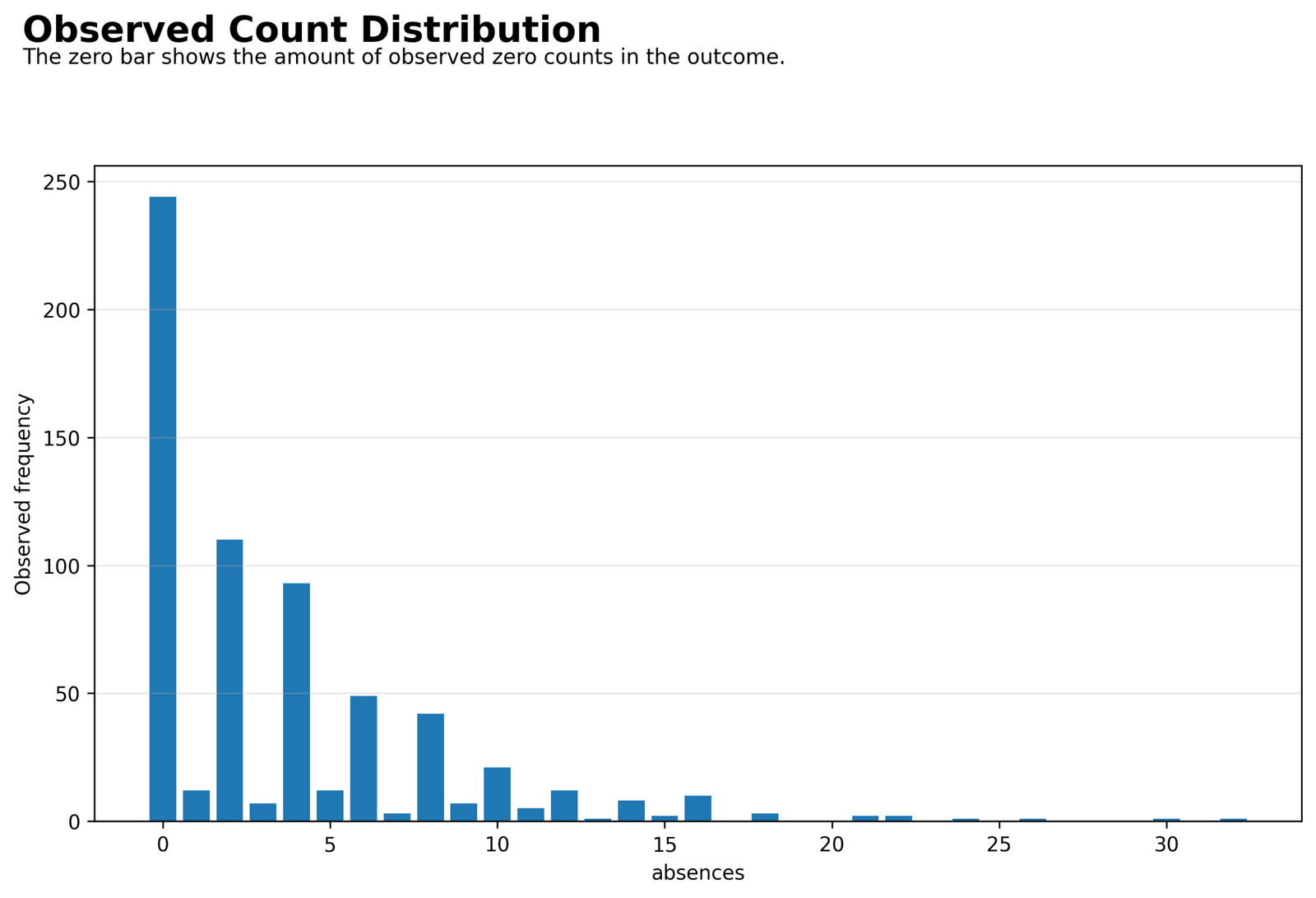
The distribution has a dominant bar at zero, a long right tail to 32, and pronounced spikes at several even counts. The positive part is not a smooth Poisson-shaped sequence.
There are 244 zeros among 649 observations. The mean is 3.6595, the variance is 21.5366, and the variance-to-mean ratio is 5.8852.
The large zero mass motivates an additional zero process. The long tail and count heaping also indicate that excess zeros are not the only departure from a simple Poisson distribution.
A ZIP model should be evaluated against both problems. Matching the zero bar is necessary, but residual and frequency checks must determine whether the Poisson count state is still too narrow.
Zero Inflated Poisson Regression — Python Chart 2: Observed Versus Expected Frequencies
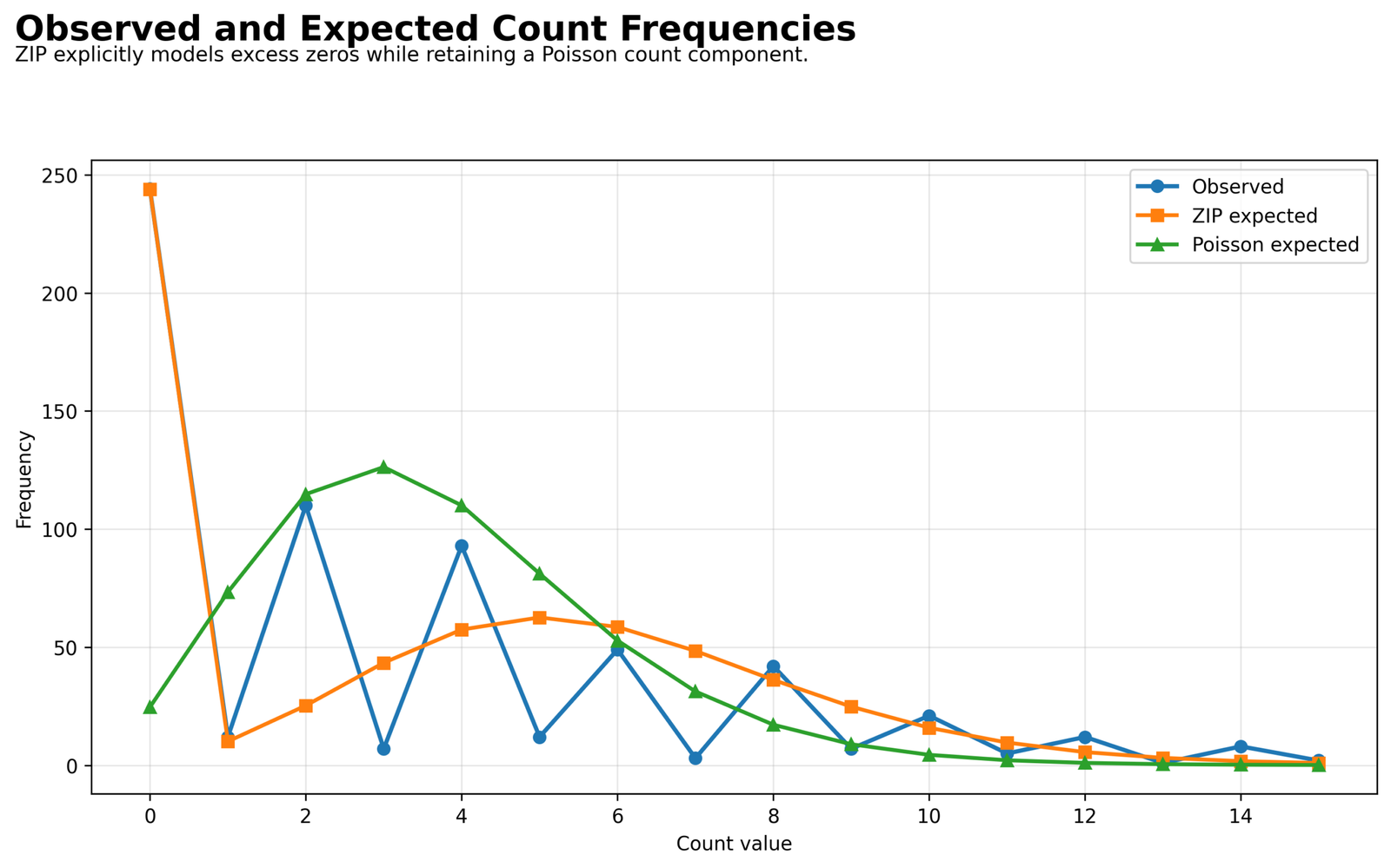
The ZIP curve rises to the observed zero spike, while standard Poisson allocates most probability around small positive counts. Beyond zero, the ZIP curve is smoother than the observed alternating spikes.
At zero, observed = 244, ZIP expected = 243.8578, and Poisson expected = 24.6591. At count 2, observed = 110 versus ZIP expected = 25.2953; at count 4, observed = 93 versus ZIP expected = 57.4578.
The mixture nearly eliminates the Poisson zero deficit but does not reproduce every positive-count frequency. The strong even-count heaping may reflect recording rules, omitted groups or a count distribution more flexible than Poisson.
The chart explains why likelihood improves dramatically while point prediction and residual diagnostics remain imperfect. Zero fit and positive-count fit must be reported separately.
Zero Inflated Poisson Regression — Python Chart 3: Count-Component Incidence Rate Ratios
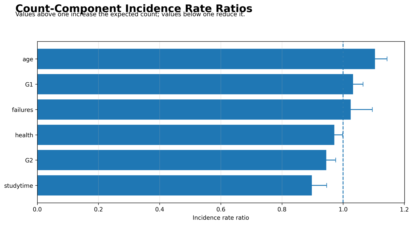
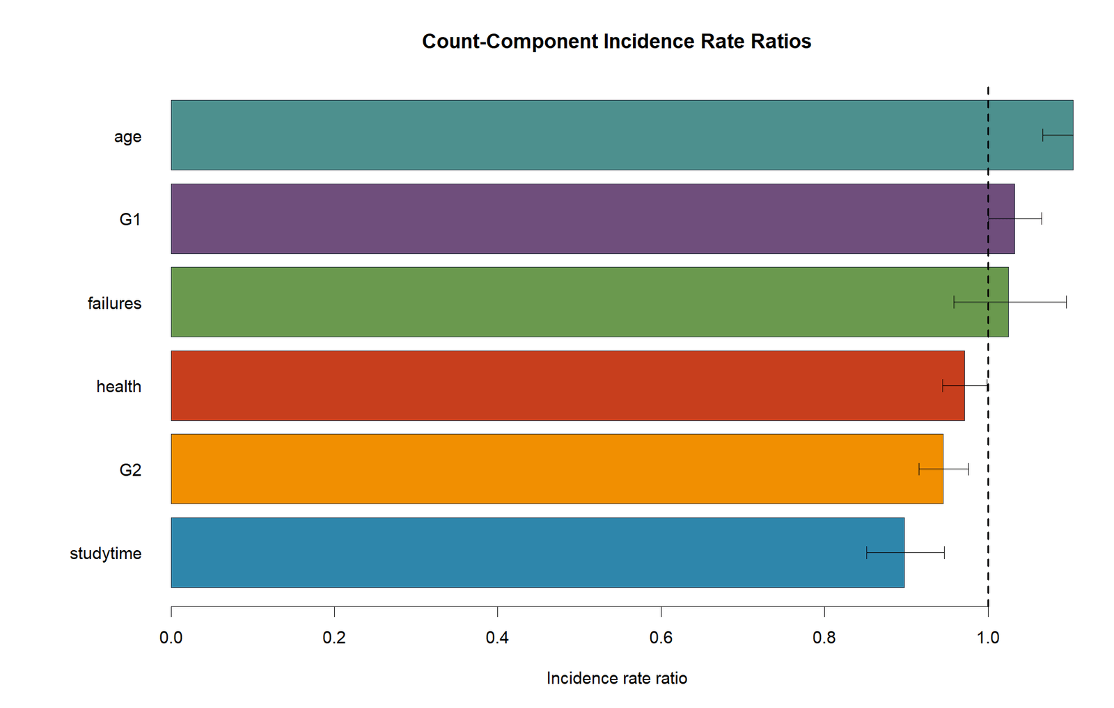
Age and G1 are above the null value of one. G2, studytime and health are below one. The failures interval crosses one.
IRRs are 1.0326 for G1, 0.9451 for G2, 0.8976 for studytime, 1.0247 for failures, 1.1044 for age and 0.9710 for health.
Holding the other count predictors fixed, age is associated with a 10.44% higher count-state mean per year, while a one-unit studytime increase is associated with about a 10.24% lower count-state mean. Failures is not individually significant in this equation.
These effects describe λ among cases in the count-generating state. They should not be described as direct effects on the unconditional mean without considering the inflation probability.
Zero Inflated Poisson Regression — Python Chart 4: Inflation-Component Odds Ratios
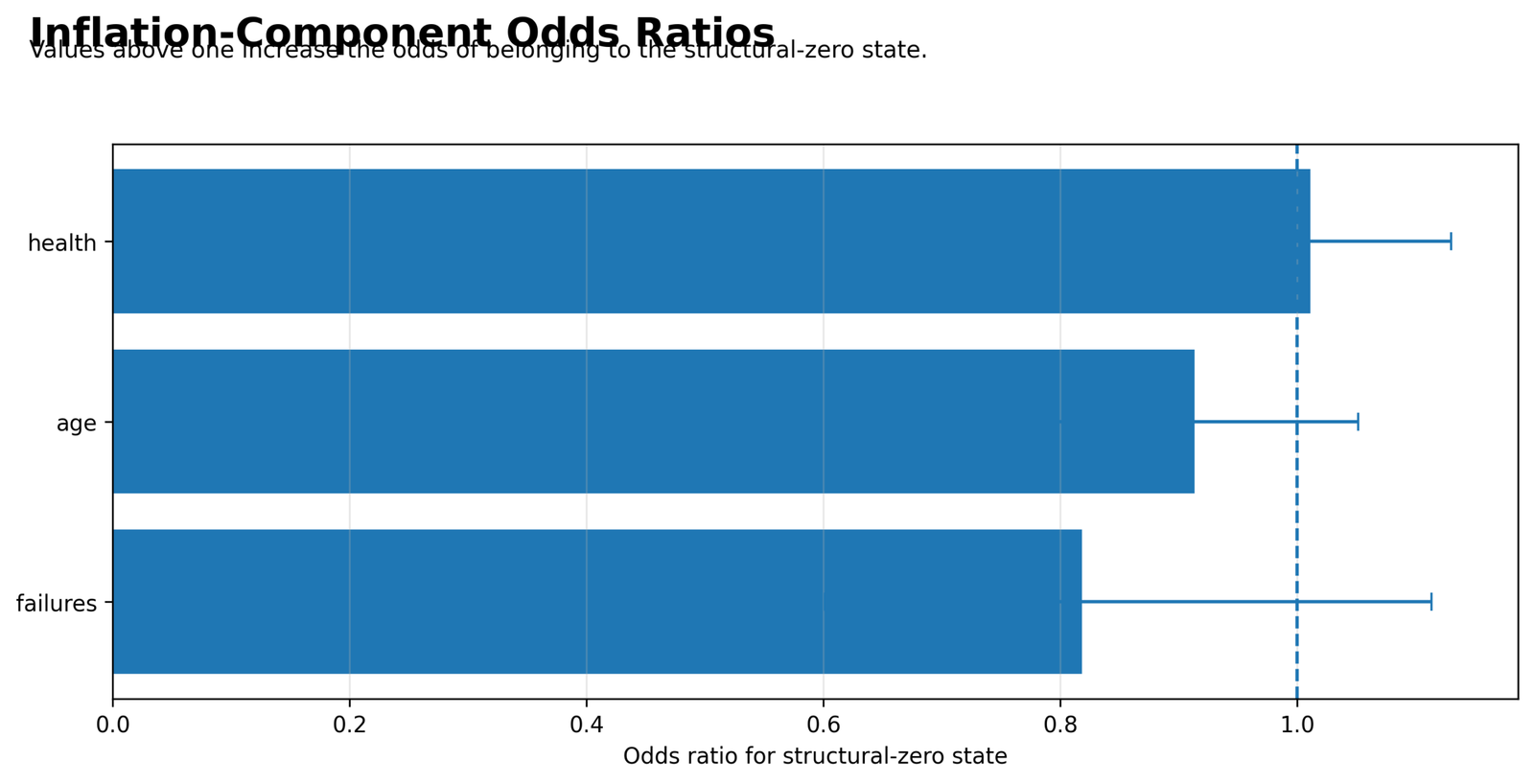
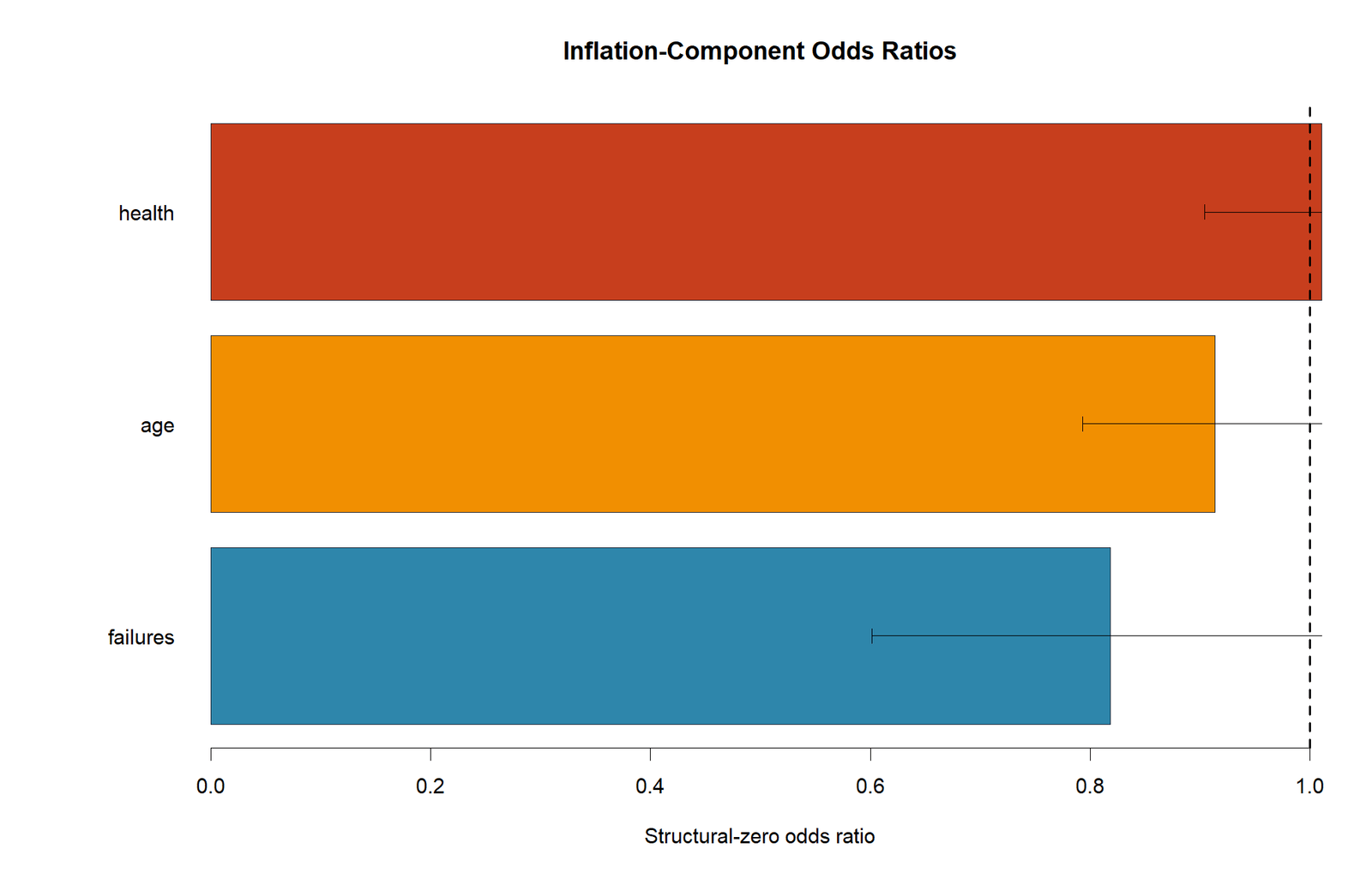
All three inflation intervals cross one. The point estimates for failures and age are below one, while health is very close to one.
Structural-zero ORs are 0.8183 for failures, 0.9134 for age and 1.0109 for health. Their p-values are .2019, .2074 and .8482.
The supplied variables do not individually distinguish structural-zero membership at α = .05. The model can still improve fit because the inflation intercept and mixture structure add probability mass to zero.
A strong overall ZIP-versus-Poisson comparison does not imply strong inflation predictors. The latent state is useful distributionally but weakly explained by these three covariates.
Zero Inflated Poisson Regression — Python Chart 5: Observed Counts Versus ZIP Predicted Means
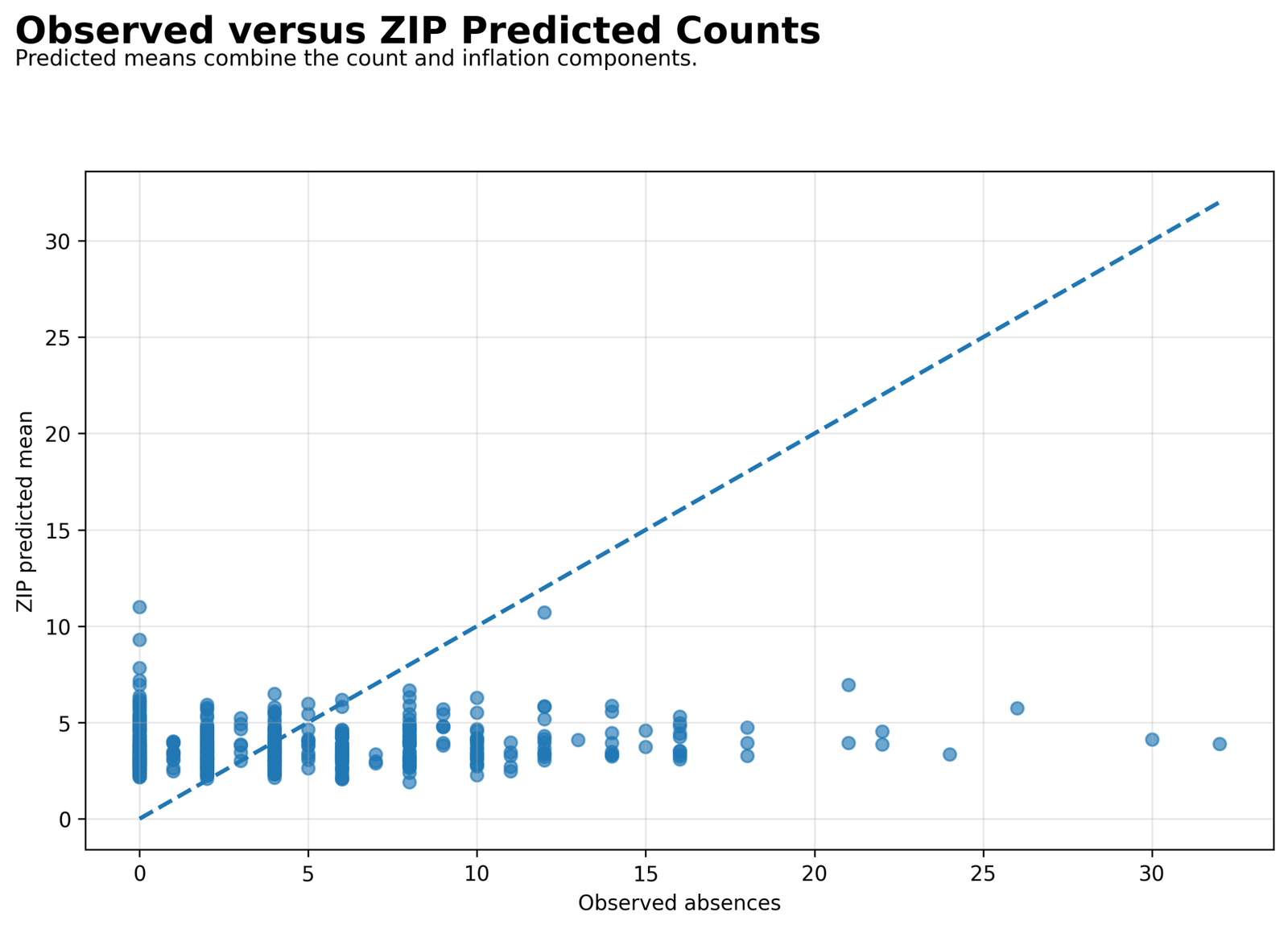
Fitted means occupy a comparatively narrow band, while observed counts extend to 32. High-count cases lie well above the equality line.
ZIP RMSE is 4.5596 and MAE is 3.3514. Standard Poisson has RMSE 4.5276 and MAE 3.3270, so ZIP is slightly worse on these in-sample point-error metrics.
The mixture improves probability allocation at zero without expanding the Poisson state enough to capture the largest positive counts. Likelihood fit and mean-prediction accuracy therefore move in different directions.
Researchers interested in individual count forecasts should not rely on AIC alone. Holdout validation and a ZINB comparison are needed before claiming predictive superiority.
Zero Inflated Poisson Regression — Python Chart 6: ZIP Pearson Residuals
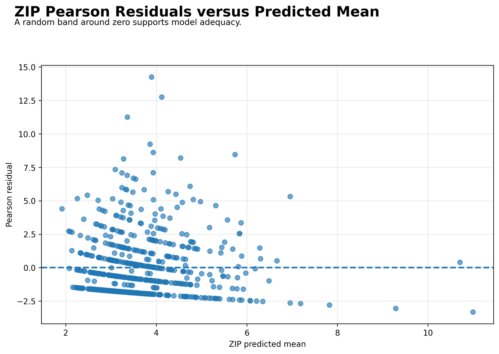
Residuals form discrete bands and show a long positive tail. Several high-count observations have residuals greater than ten.
The raw variance-to-mean ratio is 5.8852, and the largest visible residuals are far above the central residual cloud.
Zero inflation has not absorbed all extra-Poisson variation. The positive tail indicates systematic underprediction of some large counts and possible inadequacy of the Poisson variance within the count state.
This is the strongest diagnostic reason to compare Zero Inflated Poisson Regression with zero-inflated negative binomial regression and to review exposure, clustering, nonlinear effects and influential cases.
Zero Inflated Poisson Regression — Python Chart 7: Predicted Total-Zero Probability Distribution
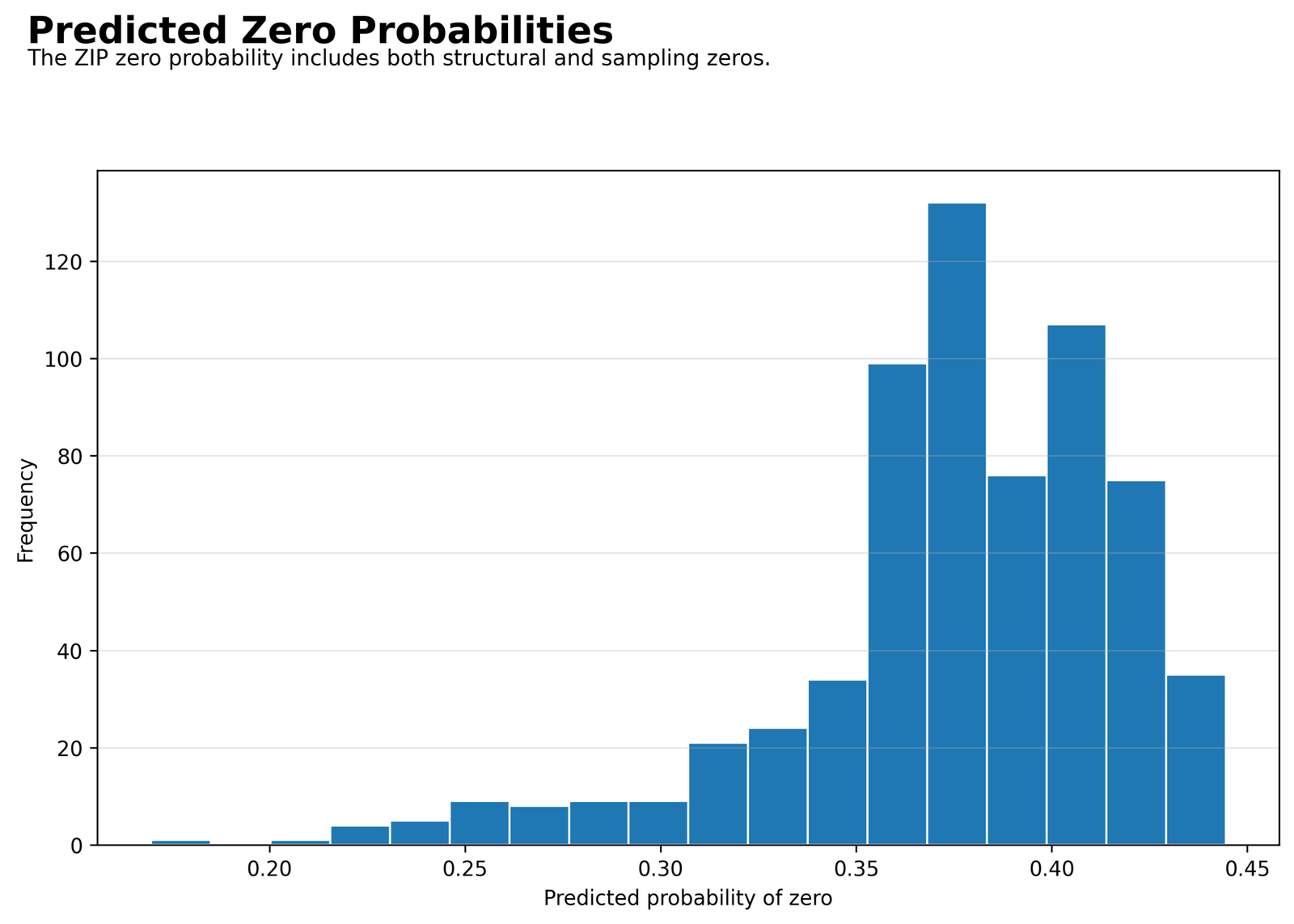
Most predicted probabilities are concentrated in a narrow middle range rather than spreading from near zero to near one.
The all-case mean total-zero probability is 0.3757 and the median is 0.3815, closely matching the observed zero proportion of 0.3760.
The model is well calibrated at the aggregate level, but the narrow probability distribution suggests limited ability to distinguish which individual cases will have zero absences.
This chart concerns total zero probability, not π alone. It combines structural-zero probability with the chance of a Poisson sampling zero.
Zero Inflated Poisson Regression — Python Chart 8: Zero Probability by Observed Outcome Status
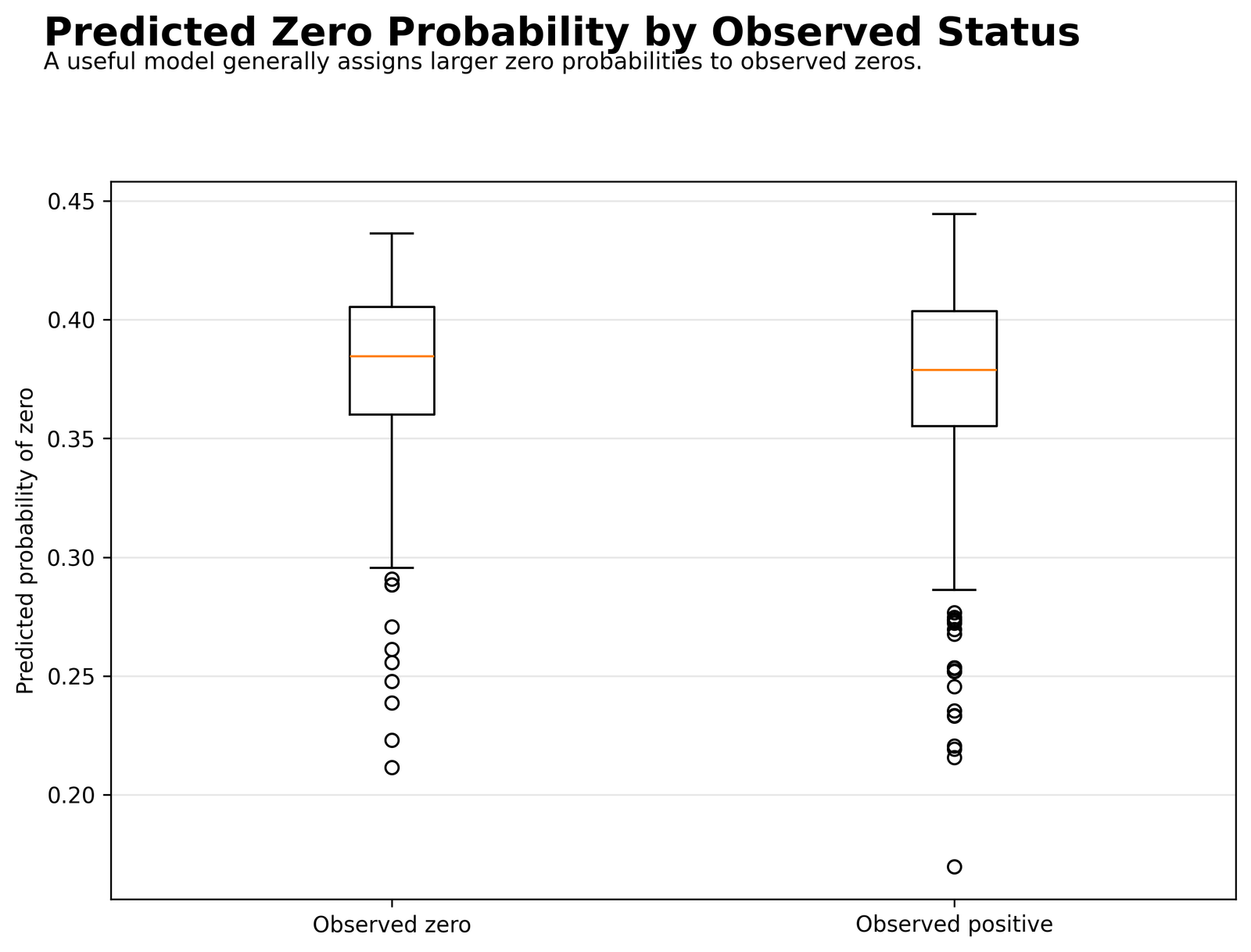
The observed-zero and observed-positive groups overlap heavily. Their centers differ only slightly.
Mean P(Y = 0) is 0.3809 for observed zeros and 0.3726 for positive counts. Medians are 0.3846 and 0.3788.
The model reproduces the correct number of zeros mainly through calibration of the overall probability mass, not through sharp case-level separation.
Calibration and discrimination are different properties. Excellent expected-zero totals should not be described as accurate classification of structural-zero cases.
Zero Inflated Poisson Regression — Python Chart 9: ZIP Versus Poisson AIC
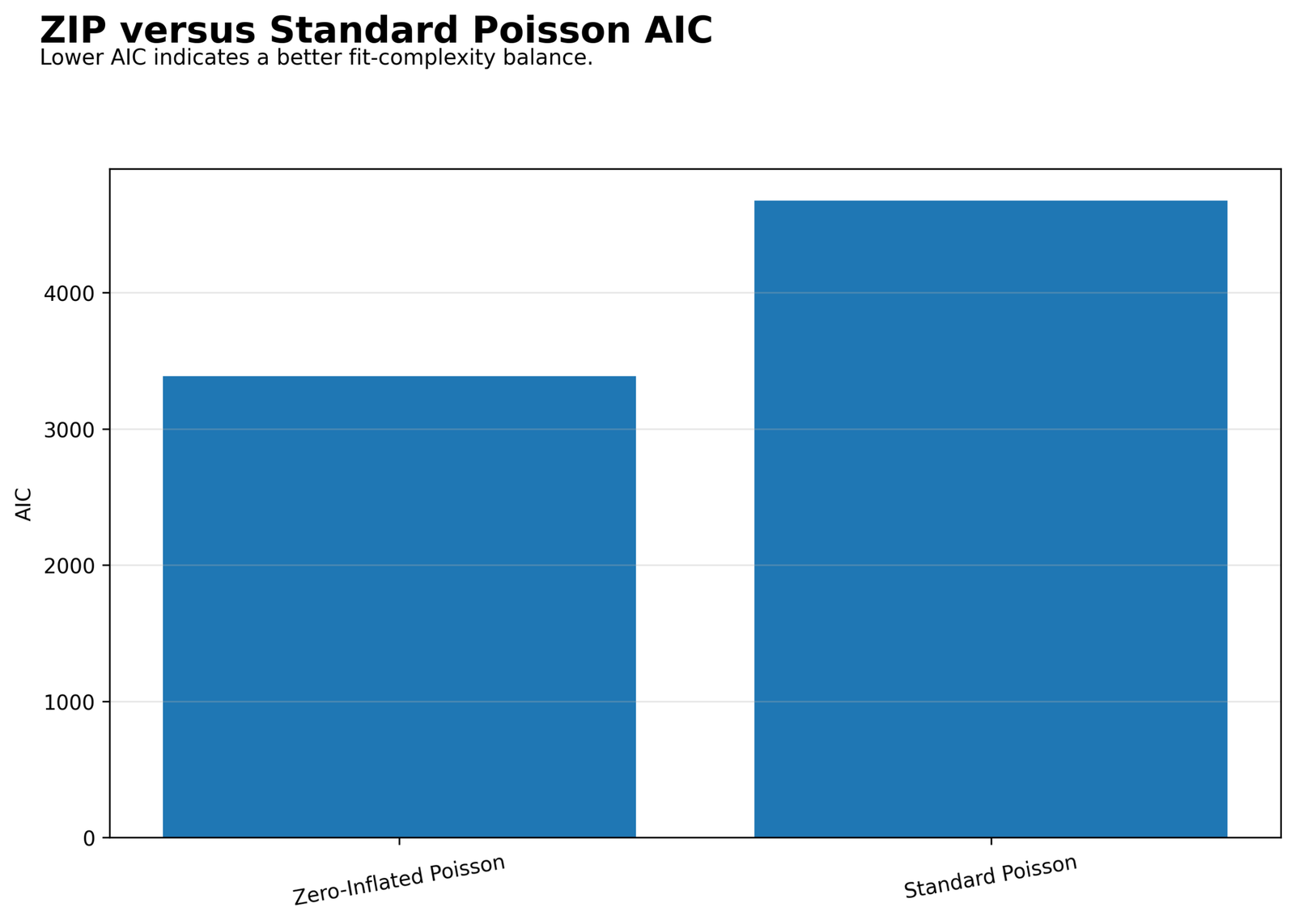
The ZIP bar is dramatically lower than the standard Poisson bar, even after penalizing the additional parameters.
ZIP AIC = 3388.4798 and Poisson AIC = 4674.7564, a difference of 1286.2765. BIC values are 3437.7096 and 4706.0844.
The probability distribution produced by ZIP is much closer to the observed data than the fitted Poisson distribution. The improvement is driven heavily by the zero mass.
Information criteria rank the supplied candidates; they do not establish that ZIP is fully adequate. Residual evidence still supports comparison with ZINB and other alternatives.
Zero Inflated Poisson Regression — Python Chart 10: Verified Model Summary
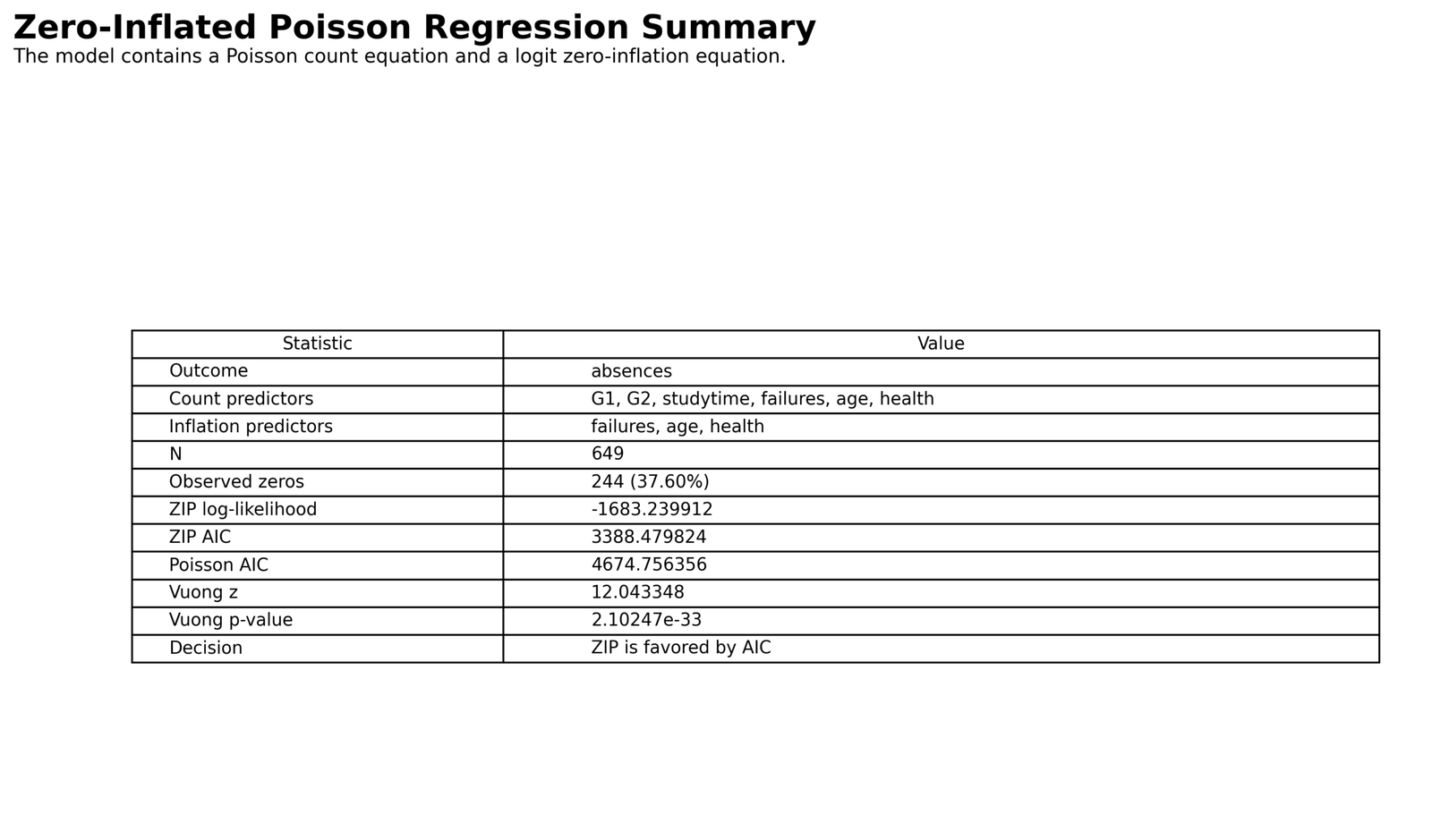
The summary consolidates sample size, zero frequency, likelihood, information criteria and the nonnested model comparison.
N = 649, zeros = 244, log likelihood = −1683.2399, AIC = 3388.4798, BIC = 3437.7096, Vuong z = 12.0433.
Every displayed value agrees with the machine-readable result tables used in the article. Together they show decisive improvement over standard Poisson for the fitted distribution.
The summary is a checkpoint, not a replacement for coefficient tables, zero calibration, residual diagnostics and the distinction between distributional fit and point prediction.
R Charts and Explanations
The R output provides an independent implementation of the same Zero Inflated Poisson Regression specification. The four available R charts are paired below. Cross-software validation is based on the same sample size, outcome, predictor sets, coefficient directions, likelihood values and zero-frequency conclusions.
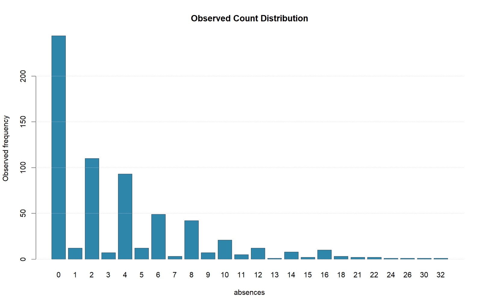
Zero Inflated Poisson Regression — R Chart 1: Observed Absence Distribution
The R distribution confirms the same dominant mass at zero and the same long positive tail. There are 244 zeros among 649 cases, while the count reaches 32. The pattern supports an inflation process but also shows why the positive-count variance requires additional scrutiny.
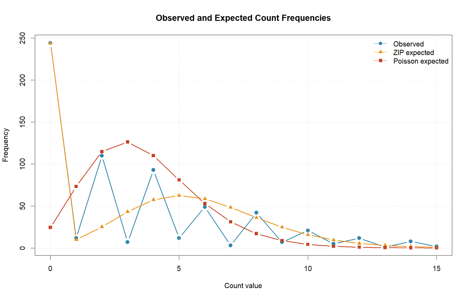
Zero Inflated Poisson Regression — R Chart 2: Observed and Expected Frequencies
The R frequency comparison reproduces the central calibration result: ZIP expects 243.8578 zeros against 244 observed, whereas standard Poisson expects 24.6591. Positive-count spikes remain imperfectly fitted, especially where the observed distribution alternates sharply between neighbouring counts.
Zero Inflated Poisson Regression — R Chart 3: Count-State Incidence Rate Ratios
The R coefficient plot confirms the count-state directions and uncertainty. Age has IRR 1.1044, G1 has 1.0326, G2 has 0.9451, studytime has 0.8976, health has 0.9710 and failures has 1.0247. All except failures meet the supplied .05 rule.
Zero Inflated Poisson Regression — R Chart 4: Structural-Zero Odds Ratios
The R inflation plot confirms that failures, age and health do not have individually significant structural-zero odds ratios. Their estimates are 0.8183, 0.9134 and 1.0109, and every confidence interval crosses one.
Zero Inflated Poisson Regression Coefficient and Parameter Interpretation
A Zero Inflated Poisson Regression coefficient must always be interpreted with its component and link function. Count coefficients describe the Poisson mean λ on the log scale. Inflation coefficients describe structural-zero odds on the logit scale. Exponentiating the estimates produces incidence rate ratios for the count component and odds ratios for the inflation component.
Count Component: Incidence Rate Ratios
| Term | Log-count beta | SE | z | p | IRR | IRR lower | IRR upper | Decision |
|---|---|---|---|---|---|---|---|---|
| Intercept | 0.6638512263500937 | 0.32885135242876645 | 2.018696962767981 | 0.043518725876096016 | 1.9422580244257546 | 1.019502149403972 | 3.7002042964319988 | Statistically significant |
| G1 | 0.03205984880276248 | 0.015868226621080252 | 2.0203800694510097 | 0.043343979143648764 | 1.0325793020908556 | 1.0009591558229485 | 1.0651983239314446 | Statistically significant |
| G2 | -0.05649644486701268 | 0.01632705682780934 | -3.460295720339757 | 0.0005395824637254096 | 0.9450698443381533 | 0.9153059589595443 | 0.9758015906425648 | Statistically significant |
| studytime | -0.10802263707344836 | 0.026862755446859145 | -4.021279100989568 | 5.788297320609825e-05 | 0.8976072769985923 | 0.8515707699175662 | 0.9461325496163061 | Statistically significant |
| failures | 0.02437807154499767 | 0.03416523731611619 | 0.7135343834857021 | 0.47551514452964894 | 1.0246776461279115 | 0.9583094244616516 | 1.0956422337848495 | Not statistically significant |
| age | 0.0993201417802294 | 0.017754920256568253 | 5.593950316025042 | 2.2196049595576726e-08 | 1.1044198138938488 | 1.0666481243119976 | 1.1435290584775317 | Statistically significant |
| health | -0.029398066389284293 | 0.014333793684419541 | -2.0509620158157587 | 0.04027064594725209 | 0.9710298531756887 | 0.9441296456501991 | 0.9986965032848301 | Statistically significant |
Positive count-state associations
- G1: IRR = 1.0326, 95% CI [1.0010, 1.0652], p = .0433. Each one-unit increase is associated with a 3.26% higher count-state mean.
- Age: IRR = 1.1044, 95% CI [1.0666, 1.1435], p < .001. Each additional year is associated with a 10.44% higher count-state mean.
Negative count-state associations
- G2: IRR = 0.9451, 95% CI [0.9153, 0.9758], p < .001, corresponding to about a 5.49% lower count-state mean per unit.
- studytime: IRR = 0.8976, 95% CI [0.8516, 0.9461], p < .001, corresponding to about a 10.24% lower count-state mean per unit.
- health: IRR = 0.9710, 95% CI [0.9441, 0.9987], p = .0403, corresponding to about a 2.90% lower count-state mean per unit.
The failures coefficient is 0.0244, giving IRR = 1.0247, 95% CI [0.9583, 1.0956], p = .4755. The interval includes one, so the analysis does not support an individual count-state failures effect after adjustment for the other predictors. The count intercept has IRR 1.9423, but a profile with age, grades, studytime, failures and health all equal to zero is not substantively realistic. Centering continuous predictors would make the intercept easier to interpret without changing fitted values.
Inflation Component: Structural-Zero Odds Ratios
| Term | Logit gamma | SE | z | p | Structural-zero OR | OR lower | OR upper | Decision |
|---|---|---|---|---|---|---|---|---|
| Intercept | 0.9972672581991876 | 1.2150943291301504 | 0.8207323779653398 | 0.41179872385469396 | 2.7108636067388483 | 0.2505056347458572 | 29.335793192023964 | Not statistically significant |
| failures | -0.2005682516041767 | 0.1571632883155433 | -1.2761774950997937 | 0.20189278215654172 | 0.8182656401772482 | 0.6013352760238732 | 1.113453150997415 | Not statistically significant |
| age | -0.09063237063640193 | 0.07188913209681388 | -1.2607242290023244 | 0.20740822137761805 | 0.9133534247246264 | 0.7933169278128857 | 1.0515526004923021 | Not statistically significant |
| health | 0.010880677532247498 | 0.05683068770350098 | 0.1914577840235639 | 0.8481669521517261 | 1.0109400873816496 | 0.9043802074181175 | 1.130055536258238 | Not statistically significant |
The failures inflation coefficient is −0.2006, giving OR = 0.8183, 95% CI [0.6013, 1.1135], p = .2019. The age coefficient is −0.0906, giving OR = 0.9134, 95% CI [0.7933, 1.0516], p = .2074. The health coefficient is 0.0109, giving OR = 1.0109, 95% CI [0.9044, 1.1301], p = .8482. None of these confidence intervals excludes one.
The lack of individually significant inflation slopes does not contradict the model-level evidence. The extra component can improve the likelihood through its intercept and mixture structure while the selected inflation predictors explain little variation in π across cases. This is exactly what the narrow predicted-zero probability distribution and heavy group overlap suggest.
Conditional and Unconditional Effects Are Not Identical
An IRR is a conditional effect on λ, not automatically a percentage change in the final expected outcome μ = (1 − π)λ. A predictor appearing only in the count equation changes μ through λ. A predictor appearing only in the inflation equation changes μ through π. A predictor appearing in both equations can have competing effects, so its overall marginal effect depends on the profile at which it is evaluated.
Predictions, Effects and Model Meaning
Zero Inflated Poisson Regression produces several predictions for each observation. The count-state linear predictor is η = x′β. Exponentiating η gives λ, the expected count for a case known to be in the Poisson state. The inflation linear predictor is z′γ, which becomes π after the logistic transformation. The final expected count is μ = (1 − π)λ, and the total zero probability is π + (1 − π)e−λ.
| Quantity | Formula | Meaning | Common error |
|---|---|---|---|
| Count linear predictor | η = x′β | Log of the Poisson mean in the count state | Reading η as a count without exponentiating |
| Count-state mean | λ = exp(η) | Expected count conditional on being in the count state | Calling λ the unconditional fitted count |
| Structural-zero probability | π = logistic(z′γ) | Probability of membership in the always-zero state | Calling π the complete probability of observing zero |
| Unconditional expected count | μ = (1 − π)λ | Expected observed count after combining both states | Ignoring the inflation component in prediction |
| Total zero probability | π + (1 − π)e−λ | Probability that the observed count equals zero | Assuming every predicted zero is structural |
What the Worked Zero Inflated Poisson Regression Predictions Show
The model’s average predicted total-zero probability is 0.3757, essentially matching the observed zero proportion of 0.3760. Summing the case-level zero probabilities gives 243.8578 expected zeros, compared with 244 observed. This is strong aggregate calibration.
Case-level discrimination is much weaker. Mean predicted zero probability is 0.3809 among observed-zero cases and 0.3726 among positive cases. Because the two distributions overlap heavily, a threshold rule would not reliably identify which students will have zero absences. The model is better understood as a probability-distribution model than as a zero classifier.
The unconditional predicted means are also compressed relative to the observed range. Counts reach 32, but the fitted means remain much lower for many high-count cases. This underprediction contributes to ZIP RMSE of 4.5596 and MAE of 3.3514. Those values are slightly larger than the standard Poisson errors, despite ZIP’s much stronger likelihood and information criteria.
Marginal Effects
For a count-only predictor, the derivative of μ with respect to that predictor is proportional to β(1 − π)λ. For an inflation-only predictor, the effect operates through the derivative of π and generally moves the expected count in the opposite direction of the structural-zero odds. When a predictor occurs in both components, both pathways must be combined.
Average marginal effects are usually easier to communicate than component coefficients because they summarize change on the observed-count scale. They should be calculated for each case and averaged, or evaluated at clearly stated representative profiles. The supplied output emphasizes IRRs, odds ratios and fitted probabilities; it should not be described as containing average marginal effects unless those derivatives are explicitly generated.
Zero Inflated Poisson Regression Assumptions and Diagnostics
Zero Inflated Poisson Regression should be judged as a complete probability model, not only by convergence or a lower AIC. The analysis requires a meaningful count outcome, independent observations unless dependence is modelled, appropriate link functions, correct functional form, a plausible extra-zero mechanism and an adequate Poisson variance within the count state.
1. Count Outcome and Exposure
Absences is a nonnegative integer outcome, satisfying the basic count requirement. The model does not include an offset, so it assumes comparable opportunity for absences across students. Unequal observation windows would require log exposure in the count equation. Without that adjustment, coefficients would mix event rate with time at risk.
2. Excess-Zero Evidence
The strongest support for an additional zero process is the fitted Poisson zero deficit. Standard Poisson expects 24.6591 zeros, whereas 244 are observed. Zero Inflated Poisson Regression expects 243.8578. This is much stronger evidence than the raw zero percentage alone because it evaluates zeros relative to the fitted count mean.
3. Remaining Count-State Dispersion
The observed variance is 21.5366 and the mean is 3.6595, producing a variance-to-mean ratio of 5.8852. Some of that excess variance is created by the zero mass, but the residual plot retains a long positive tail after fitting ZIP. High counts are systematically underpredicted, so the Poisson state remains questionable.
4. Functional Form
The model assumes linear relationships on the log-count and logit scales. G1, G2, studytime, failures, age and health enter without nonlinear terms or interactions. The effect of a one-unit age increase is therefore assumed constant on each relevant link scale. Residual patterns, partial-effect plots, splines or polynomial comparisons should be used to test that simplification.
5. Independence and Clustering
The likelihood treats all 649 observations as independent. Students may share school, class, household or other contextual influences. Ignoring clustering can understate uncertainty and can create apparent overdispersion or zero inflation. Cluster-robust standard errors, generalized estimating equations or mixed zero-inflated models may be needed when the design contains grouped observations.
6. Identifiability of the Inflation State
Structural-zero membership is latent. The model separates the two processes through distributional shape and predictor information, not observed labels. Here, the zero probabilities for observed-zero and positive groups are very similar, and no inflation slope is individually significant. That pattern suggests weak covariate separation even though the mixture substantially improves overall calibration.
7. Residuals and Influential Cases
Pearson residuals show several extreme positive values above ten. Those cases should be inspected for data-entry problems, unusual exposure, omitted predictors and genuine high-risk profiles. Influence should be assessed by refitting after removal or by using case-deletion measures; automatically deleting high counts would bias the analysis.
8. Count Heaping
Observed frequencies alternate sharply, with large spikes at several even counts and small frequencies at neighbouring odd counts. Heaping can arise from rounding, reporting conventions or a discrete schedule. A smooth Poisson mixture cannot reproduce that mechanism exactly. Sensitivity analyses may require grouped-count models or explicit heaping processes when the pattern is substantive.
9. Calibration and Discrimination
Aggregate zero calibration is excellent because the mean predicted zero probability closely matches the observed zero proportion. Discrimination is weak because observed-zero and positive groups overlap. Both properties should be reported; matching the expected number of zeros does not imply accurate identification of individual structural-zero cases.
10. External Validation
AIC, BIC, likelihood, Vuong statistics, RMSE and MAE in this article are calculated on the fitted sample. External validation should reproduce the full prediction process on untouched data, including λ, π, the unconditional mean and total zero probability. Calibration of zero probabilities and error for positive counts should be assessed separately.
243.8578 expected zeros versus 244 observed.
Mean zero probabilities differ by only about 0.0082 between outcome groups.
High counts and Pearson residuals show remaining extra-Poisson variation.
Zero Inflated Poisson Regression in Python, R, SPSS and Excel
The four software resources serve different purposes. Python and R fit the two-equation likelihood directly and provide the most complete diagnostics. SPSS output offers an additional implementation route and archived evidence. Excel exposes the prediction arithmetic but should not be treated as the preferred engine for maximum-likelihood estimation or covariance calculations.
Python workflow
- Read
dataset.csvand retain complete records for absences and all predictors. - Create separate count and inflation design matrices with intercepts.
- Fit
ZeroInflatedPoissonby maximum likelihood and fit standard Poisson as the comparison. - Export β, γ, IRRs, odds ratios, fitted means, zero probabilities, expected frequencies and residuals.
- Calculate AIC, BIC, Vuong statistics, RMSE, MAE and expected zeros.
Python is the displayed chart source for this article. Its output supplies the ten visual diagnostics and all exact values used in the worked interpretation.
R workflow
- Fit the count and inflation formulas with a zero-inflated count-model package.
- Confirm the direction and scale of the inflation parameterization before interpreting odds ratios.
- Export count coefficients, inflation coefficients, model fit and case-level predictions.
- Compare ZIP with Poisson and, where available, ZINB using likelihood and information criteria.
- Reproduce frequency, coefficient and diagnostic plots.
The R report independently confirms the main Zero Inflated Poisson Regression findings and provides the four paired charts shown above.
SPSS workflow
- Verify that the procedure or extension supports a true two-component zero-inflated model.
- Define absences as the count response and specify the log and logit equations separately.
- Use the same predictors and reference coding as the Python and R analyses.
- Save parameter estimates, covariance output, fit criteria and case-level predictions.
- Confirm whether the inflation model represents structural-zero probability or count-state probability.
SPSS results should not be mixed with coefficients from a different parameterization. Directional agreement must be checked after confirming how the software defines the inflation component.
Excel workflow
- Enter fitted β and γ values in clearly labelled cells.
- Calculate count η, λ, inflation logit, π, unconditional mean and total zero probability for each row.
- Compute observed residuals and compare expected zero totals with the fitted report.
- Protect coefficient cells and document all raw-variable coding.
- Use Excel for audit and teaching rather than as a substitute for likelihood optimization.
The worked workbook makes the mixture formulas transparent and allows row-by-row verification of the final predictions.
Code: Expand Only the Software You Need
Python Zero Inflated Poisson Regression source excerpt
# -*- coding: utf-8 -*-
r"""
Zero Inflated Poisson Regression - Python Output Generator

- Reads dataset.csv from the script folder first, then BASE_DIR fallback.
- Creates Python_Output/png, Python_Output/csv, Python_Output/txt, and Python_Output/pdf.
- Cleans old outputs before regenerating.
- Fits a Zero-Inflated Poisson model and a standard Poisson comparison model.
- Default count outcome: absences.
- Default count predictors: G1, G2, studytime, failures, age, health.
- Default inflation predictors: failures, age, health.
- Generates PNG charts, CSV tables, TXT report, and PDF report.
"""

from __future__ import annotations

from pathlib import Path
import os
import warnings
warnings.filterwarnings("ignore")

import matplotlib
matplotlib.use("Agg")
import matplotlib.pyplot as plt
from matplotlib.backends.backend_pdf import PdfPages
import numpy as np
import pandas as pd
from scipy import stats
import statsmodels.api as sm
from statsmodels.discrete.count_model import ZeroInflatedPoisson

TEST_NAME = "Zero Inflated Poisson Regression"
BASE_DIR = Path(os.environ.get(
    "ANALYSIS_BASE_DIR",
    r"analysis-folder",
))
OUTCOME_DEFAULT = "absences"
COUNT_PREDICTORS_DEFAULT = ["G1", "G2", "studytime", "failures", "age", "health"]
INFLATION_PREDICTORS_DEFAULT = ["failures", "age", "health"]
ALPHA = 0.05

OUTPUT_DIR = BASE_DIR / "Python_Output"
PNG_DIR = OUTPUT_DIR / "png"
CSV_DIR = OUTPUT_DIR / "csv"
TXT_DIR = OUTPUT_DIR / "txt"
PDF_DIR = OUTPUT_DIR / "pdf"

for folder in (OUTPUT_DIR, PNG_DIR, CSV_DIR, TXT_DIR, PDF_DIR):
    folder.mkdir(parents=True, exist_ok=True)


def cleanup_outputs() -> None:
    for folder in (PNG_DIR, CSV_DIR, TXT_DIR, PDF_DIR):
        for pattern in ("*.png", "*.csv", "*.txt", "*.pdf"):
            for item in folder.glob(pattern):
                try:
                    item.unlink()
                except OSError:
                    pass
    (OUTPUT_DIR / "00_PYTHON_SCRIPT_STARTED.txt").write_text(
        "Zero Inflated Poisson Regression Python script started successfully.\n",
        encoding="utf-8",
    )


def find_dataset(base_dir: Path) -> Path:
    script_dir = Path(__file__).resolve().parent
    candidates = [
        script_dir / "dataset.csv",
        script_dir / "dataset",
        script_dir / "dataset.txt",
        base_dir / "dataset.csv",
        base_dir / "dataset",
        base_dir / "dataset.txt",
    ]
    for candidate in candidates:
        if candidate.exists():
            return candidate
    raise FileNotFoundError(
        f"No dataset found. Expected dataset.csv in the script folder or {base_dir}."
    )


def read_dataset(path: Path) -> pd.DataFrame:
    for sep in (",", ";", "\t"):
        try:
            frame = pd.read_csv(path, sep=sep)
            if frame.shape[1] > 1:
                frame.columns = [str(c).strip() for c in frame.columns]
                return frame
        except Exception:
            continue
    frame = pd.read_csv(path)
    frame.columns = [str(c).strip() for c in frame.columns]
    return frame


def numeric_usable(series: pd.Series, min_n: int = 10) -> bool:
    values = pd.to_numeric(series, errors="coerce").dropna()
    return (
        len(values) >= min_n
        and values.nunique() > 1
        and np.isfinite(values.std())
        and values.std() > 0
    )


def choose_outcome(df: pd.DataFrame) -> str:
    if OUTCOME_DEFAULT in df.columns and numeric_usable(df[OUTCOME_DEFAULT]):
        return OUTCOME_DEFAULT
    candidates = []
    for name in df.columns:
        if not numeric_usable(df[name]):
            continue
        values = pd.to_numeric(df[name], errors="coerce").dropna()
        if np.all(values >= 0) and np.allclose(values, np.round(values)):
            candidates.append(name)
    if not candidates:
        raise ValueError("No usable non-negative count outcome was found.")
    return candidates[0]


def choose_predictors(
    df: pd.DataFrame,
    outcome: str,
    preferred: list[str],
    limit: int,
) -> list[str]:
    selected: list[str] = []
    for name in preferred:
        if name in df.columns and name != outcome and numeric_usable(df[name]):
            selected.append(name)
    for name in df.columns:
        if len(selected) >= limit:
            break
        if name == outcome or name in selected:
            continue
        if numeric_usable(df[name]):
            selected.append(name)
    if len(selected) < 1:
        raise ValueError("No usable numeric predictors were found.")
    return selected[:limit]


def prepare_data(df: pd.DataFrame):
    outcome = choose_outcome(df)
    count_predictors = choose_predictors(
        df, outcome, COUNT_PREDICTORS_DEFAULT, 6
    )
    inflation_predictors = [
        p for p in INFLATION_PREDICTORS_DEFAULT
        if p in count_predictors or (p in df.columns and numeric_usable(df[p]))
    ]
    if not inflation_predictors:
        inflation_predictors = count_predictors[: min(3, len(count_predictors))]

    columns = [outcome] + list(dict.fromkeys(count_predictors + inflation_predictors))
    data = df[columns].copy()
    for name in data.columns:
        data[name] = pd.to_numeric(data[name], errors="coerce")
    data = data.replace([np.inf, -np.inf], np.nan).dropna().reset_index(drop=True)

    data[outcome] = np.round(data[outcome]).astype(int)
    data = data[data[outcome] >= 0].reset_index(drop=True)
    if len(data) <= len(count_predictors) + len(inflation_predictors) + 10:
        raise ValueError("Not enough complete observations for Zero-Inflated Poisson Regression.")
    if int((data[outcome] == 0).sum()) == 0:
        raise ValueError("The selected count outcome contains no zero observations.")

    return data, outcome, count_predictors, inflation_predictors


def fit_models(data, outcome, count_predictors, inflation_predictors):
    y = data[outcome].astype(int)
    x_count = sm.add_constant(
        data[count_predictors].astype(float), has_constant="add"
    )
    x_infl = sm.add_constant(
        data[inflation_predictors].astype(float), has_constant="add"
    )

    poisson = sm.GLM(y, x_count, family=sm.families.Poisson()).fit()

    zip_model = ZeroInflatedPoisson(
        endog=y,
        exog=x_count,
        exog_infl=x_infl,
        inflation="logit",
    )
    methods = ["bfgs", "lbfgs", "newton"]
    zip_result = None
    last_error = None
    for method in methods:
        try:
            candidate = zip_model.fit(
                method=method,
                maxiter=1500,
                disp=0,
            )
            zip_result = candidate
            converged = bool(candidate.mle_retvals.get("converged", True))
            if converged:
                break
        except Exception as exc:
            last_error = exc
    if zip_result is None:
        raise RuntimeError(f"Zero-Inflated Poisson fitting failed: {last_error}")

    return y, x_count, x_infl, poisson, zip_result


def split_coefficients(zip_result, count_predictors, inflation_predictors):
    params = zip_result.params
    bse = zip_result.bse
    pvalues = zip_result.pvalues
    conf = zip_result.conf_int(alpha=ALPHA)

    count_names = ["const"] + count_predictors
    inflation_names = ["inflate_const"] + [f"inflate_{p}" for p in inflation_predictors]

    count_rows = []
    for name in count_names:
        beta = float(params[name])
        se = float(bse[name])
        p = float(pvalues[name])
        low = float(conf.loc[name, 0])
        high = float(conf.loc[name, 1])
        count_rows.append({
            "term": "Intercept" if name == "const" else name,
            "coefficient_log_count": beta,
            "standard_error": se,
            "z_value": beta / se,
            "p_value": p,
            "ci95_lower_log": low,
            "ci95_upper_log": high,
            "incidence_rate_ratio": np.exp(beta),
            "irr_ci95_lower": np.exp(low),
            "irr_ci95_upper": np.exp(high),
            "decision_alpha_0_05": (
                "Statistically significant"
                if p < ALPHA else "Not statistically significant"
            ),
        })

    inflation_rows = []
    for name in inflation_names:
        beta = float(params[name])
        se = float(bse[name])
        p = float(pvalues[name])
        low = float(conf.loc[name, 0])
        high = float(conf.loc[name, 1])
        display = "Intercept" if name == "inflate_const" else name.replace("inflate_", "")
        inflation_rows.append({
            "term": display,
            "coefficient_logit_zero": beta,
            "standard_error": se,
            "z_value": beta / se,
            "p_value": p,
            "ci95_lower_logit": low,
            "ci95_upper_logit": high,
            "odds_ratio_structural_zero": np.exp(beta),
            "or_ci95_lower": np.exp(low),
            "or_ci95_upper": np.exp(high),
            "decision_alpha_0_05": (
                "Statistically significant"
                if p < ALPHA else "Not statistically significant"
            ),
        })
R Zero Inflated Poisson Regression source excerpt
# Zero Inflated Poisson Regression - R Output Generator
#
# - Reads dataset.csv from the script folder first, then BASE_DIR fallback.
# - Creates R_Output/charts, R_Output/tables, R_Output/txt, and R_Output/pdf.
# - Cleans old outputs before regenerating.
# - Fits a Zero-Inflated Poisson model using pscl::zeroinfl.
# - Fits a standard Poisson comparison model.
# - Generates colorful PNG charts, CSV tables, TXT report, and PDF report.

BASE_DIR <- Sys.getenv(
  "ANALYSIS_BASE_DIR",
  unset = "analysis-folder"
)

TEST_NAME <- "Zero Inflated Poisson Regression"
OUTCOME_DEFAULT <- "absences"
COUNT_PREDICTORS_DEFAULT <- c("G1", "G2", "studytime", "failures", "age", "health")
INFLATION_PREDICTORS_DEFAULT <- c("failures", "age", "health")
ALPHA <- 0.05

OUTPUT_DIR <- file.path(BASE_DIR, "R_Output")
CHART_DIR <- file.path(OUTPUT_DIR, "charts")
TABLE_DIR <- file.path(OUTPUT_DIR, "tables")
TXT_DIR <- file.path(OUTPUT_DIR, "txt")
PDF_DIR <- file.path(OUTPUT_DIR, "pdf")

for (folder in c(OUTPUT_DIR, CHART_DIR, TABLE_DIR, TXT_DIR, PDF_DIR)) {
  if (!dir.exists(folder)) dir.create(folder, recursive = TRUE, showWarnings = FALSE)
}

COLORS <- c(
  "#2E86AB", "#F18F01", "#C73E1D", "#6A994E",
  "#6F4E7C", "#4D908E", "#F9C74F", "#577590"
)

cleanup_outputs <- function() {
  for (folder in c(CHART_DIR, TABLE_DIR, TXT_DIR, PDF_DIR)) {
    for (pattern in c("*.png", "*.csv", "*.txt", "*.pdf")) {
      files <- Sys.glob(file.path(folder, pattern))
      if (length(files) > 0) unlink(files, force = TRUE)
    }
  }
  writeLines(
    "Zero Inflated Poisson Regression R script started successfully.",
    file.path(OUTPUT_DIR, "00_R_SCRIPT_STARTED.txt")
  )
}

find_dataset <- function(base_dir) {
  candidates <- c()
  args <- commandArgs(trailingOnly = FALSE)
  match <- grep("^--file=", args)
  if (length(match) > 0) {
    script_path <- normalizePath(
      sub("^--file=", "", args[match[1]]),
      winslash = "/",
      mustWork = FALSE
    )
    script_dir <- dirname(script_path)
    candidates <- c(
      candidates,
      file.path(script_dir, "dataset.csv"),
      file.path(script_dir, "dataset"),
      file.path(script_dir, "dataset.txt")
    )
  }
  candidates <- c(
    candidates,
    file.path(base_dir, "dataset.csv"),
    file.path(base_dir, "dataset"),
    file.path(base_dir, "dataset.txt")
  )
  for (item in candidates) if (file.exists(item)) return(item)
  stop("dataset.csv was not found in the script folder or BASE_DIR.")
}

read_dataset <- function(path) {
  for (sep in c(",", ";", "\t")) {
    attempt <- try(
      read.csv(path, sep = sep, stringsAsFactors = FALSE, check.names = FALSE),
      silent = TRUE
    )
    if (!inherits(attempt, "try-error") && ncol(attempt) > 1) {
      names(attempt) <- trimws(names(attempt))
      return(attempt)
    }
  }
  out <- read.csv(path, stringsAsFactors = FALSE, check.names = FALSE)
  names(out) <- trimws(names(out))
  out
}

numeric_usable <- function(x, min_n = 10) {
  values <- suppressWarnings(as.numeric(x))
  values <- values[is.finite(values)]
  length(values) >= min_n &&
    length(unique(values)) > 1 &&
    is.finite(sd(values)) &&
    sd(values) > 0
}

prepare_data <- function(df) {
  outcome <- if (
    OUTCOME_DEFAULT %in% names(df) &&
    numeric_usable(df[[OUTCOME_DEFAULT]])
  ) OUTCOME_DEFAULT else {
    candidates <- names(df)[sapply(df, function(x) {
      if (!numeric_usable(x)) return(FALSE)
      v <- suppressWarnings(as.numeric(x))
      v <- v[is.finite(v)]
      all(v >= 0) && all(abs(v - round(v)) < 1e-8)
    })]
    if (length(candidates) == 0) stop("No usable count outcome was found.")
    candidates[1]
  }

  count_predictors <- c()
  for (name in COUNT_PREDICTORS_DEFAULT) {
    if (name %in% names(df) && name != outcome && numeric_usable(df[[name]])) {
      count_predictors <- c(count_predictors, name)
    }
  }
  for (name in names(df)) {
    if (length(count_predictors) >= 6) break
    if (name == outcome || name %in% count_predictors) next
    if (numeric_usable(df[[name]])) count_predictors <- c(count_predictors, name)
  }

  inflation_predictors <- INFLATION_PREDICTORS_DEFAULT[
    INFLATION_PREDICTORS_DEFAULT %in% names(df)
  ]
  inflation_predictors <- inflation_predictors[
    sapply(inflation_predictors, function(name) numeric_usable(df[[name]]))
  ]
  if (length(inflation_predictors) == 0) {
    inflation_predictors <- head(count_predictors, min(3, length(count_predictors)))
  }

  columns <- unique(c(outcome, count_predictors, inflation_predictors))
  data <- df[, columns, drop = FALSE]
  for (name in names(data)) data[[name]] <- suppressWarnings(as.numeric(data[[name]]))
  data <- data[complete.cases(data), , drop = FALSE]
  data[[outcome]] <- round(data[[outcome]])
  data <- data[data[[outcome]] >= 0, , drop = FALSE]
  rownames(data) <- NULL

  if (sum(data[[outcome]] == 0) == 0) {
    stop("The selected outcome contains no zero observations.")
  }

  list(
    data = data,
    outcome = outcome,
    count_predictors = unique(count_predictors),
    inflation_predictors = unique(inflation_predictors)
  )
}

safe_name <- function(x) paste0("`", gsub("`", "", x), "`")

make_formula <- function(outcome, count_predictors, inflation_predictors) {
  count_rhs <- paste(safe_name(count_predictors), collapse = " + ")
  infl_rhs <- paste(safe_name(inflation_predictors), collapse = " + ")
  as.formula(paste(
    safe_name(outcome), "~", count_rhs, "|", infl_rhs
  ))
}

coefficient_tables <- function(model) {
  s <- summary(model)
  count <- as.data.frame(s$coefficients$count)
  count$term <- rownames(count)
  rownames(count) <- NULL
  names(count)[1:4] <- c("coefficient_log_count", "standard_error", "z_value", "p_value")
  count$ci95_lower_log <- count$coefficient_log_count - qnorm(0.975) * count$standard_error
  count$ci95_upper_log <- count$coefficient_log_count + qnorm(0.975) * count$standard_error
  count$incidence_rate_ratio <- exp(count$coefficient_log_count)
  count$irr_ci95_lower <- exp(count$ci95_lower_log)
  count$irr_ci95_upper <- exp(count$ci95_upper_log)
  count$decision_alpha_0_05 <- ifelse(
    count$p_value < ALPHA,
    "Statistically significant",
    "Not statistically significant"
  )
  count$term <- ifelse(count$term == "(Intercept)", "Intercept", gsub("`", "", count$term))
  count <- count[, c(
    "term", "coefficient_log_count", "standard_error", "z_value", "p_value",
    "ci95_lower_log", "ci95_upper_log", "incidence_rate_ratio",
    "irr_ci95_lower", "irr_ci95_upper", "decision_alpha_0_05"
  )]

  infl <- as.data.frame(s$coefficients$zero)
  infl$term <- rownames(infl)
  rownames(infl) <- NULL
  names(infl)[1:4] <- c("coefficient_logit_zero", "standard_error", "z_value", "p_value")
  infl$ci95_lower_logit <- infl$coefficient_logit_zero - qnorm(0.975) * infl$standard_error
  infl$ci95_upper_logit <- infl$coefficient_logit_zero + qnorm(0.975) * infl$standard_error
  infl$odds_ratio_structural_zero <- exp(infl$coefficient_logit_zero)
  infl$or_ci95_lower <- exp(infl$ci95_lower_logit)
  infl$or_ci95_upper <- exp(infl$ci95_upper_logit)
  infl$decision_alpha_0_05 <- ifelse(
    infl$p_value < ALPHA,
    "Statistically significant",
    "Not statistically significant"
  )
  infl$term <- ifelse(infl$term == "(Intercept)", "Intercept", gsub("`", "", infl$term))
  infl <- infl[, c(
    "term", "coefficient_logit_zero", "standard_error", "z_value", "p_value",
    "ci95_lower_logit", "ci95_upper_logit", "odds_ratio_structural_zero",
    "or_ci95_lower", "or_ci95_upper", "decision_alpha_0_05"
  )]

  list(count = count, inflation = infl)
}

expected_frequencies <- function(model, poisson, data, outcome) {
  y <- data[[outcome]]
  max_count <- max(y)
  lambda <- predict(model, type = "count")
  pi_zero <- predict(model, type = "zero")
  poisson_mu <- fitted(poisson)

  rows <- lapply(0:max_count, function(k) {
    zip_prob <- if (k == 0) {
      pi_zero + (1 - pi_zero) * dpois(0, lambda)
    } else {
      (1 - pi_zero) * dpois(k, lambda)
    }
    data.frame(
      count_value = k,
      observed_frequency = sum(y == k),
      expected_zip_frequency = sum(zip_prob),
      expected_poisson_frequency = sum(dpois(k, poisson_mu)),
      stringsAsFactors = FALSE
    )
  })
  do.call(rbind, rows)
}

save_chart <- function(filename, plot_function, width = 11, height = 7) {
  path <- file.path(CHART_DIR, filename)
  png(path, width = width, height = height, units = "in", res = 180)
  tryCatch(
    plot_function(),
    error = function(e) {
      plot.new()
      title(main = paste("Chart generation failed:", filename))
      text(0.05, 0.85, e$message, adj = c(0, 1))
    },
    finally = dev.off()
  )
  path
}

create_charts <- function(
  data, outcome, count_coef, infl_coef, comparison, frequency,
  predictions, model_summary
) {
  paths <- c()

  paths <- c(paths, save_chart("01_observed_count_distribution.png", function() {
    counts <- table(data[[outcome]])
    barplot(
      counts, col = COLORS[1], border = "#1F2937",
      xlab = outcome, ylab = "Observed frequency",
Advanced Zero Inflated Poisson Regression Topics
The following panels extend the worked analysis beyond the basic coefficient table. They cover model selection, latent-state meaning, prediction scales, dispersion, data structure, diagnostics, validation and reporting decisions that commonly determine whether Zero Inflated Poisson Regression is defensible.
Zero Inflated Poisson Regression: 1. ZIP Versus Standard Poisson
Standard Poisson assumes one count-generating process and assigns every zero to the Poisson distribution. Zero Inflated Poisson Regression adds a second state that always produces zero. In the worked data, Poisson expects only 24.6591 zeros, whereas ZIP expects 243.8578 against 244 observed.
The AIC difference of 1286.2765 strongly favors ZIP for the fitted distribution. The comparison does not show that every aspect of ZIP is adequate; it shows that the one-process Poisson model is unable to represent the zero mass.
Zero Inflated Poisson Regression: 2. ZIP Versus Negative Binomial Regression
Negative binomial regression handles overdispersion by adding a dispersion parameter to one count process. It can produce more zeros than Poisson indirectly because its variance is larger, but it does not posit a separate always-zero state.
Compare Zero Inflated Poisson Regression with negative binomial regression when the substantive case for structural zeros is uncertain. A negative binomial model may be more parsimonious if extra zeros are simply one consequence of broad count heterogeneity.
Zero Inflated Poisson Regression: 3. ZIP Versus Zero-Inflated Negative Binomial Regression
Zero-inflated negative binomial regression retains the structural-zero mixture and replaces the Poisson count state with a negative binomial state. It is designed for data containing both excess zeros and extra-Poisson variation among positive counts.
The variance-to-mean ratio of 5.8852 and the long positive residual tail make ZINB a particularly important sensitivity model here. Zero Inflated Poisson Regression should not be selected as final until the dispersion parameter and information criteria from ZINB are examined.
Zero Inflated Poisson Regression: 4. ZIP Versus a Hurdle Model
A hurdle model uses a binary equation for zero versus positive and a zero-truncated count model for positive outcomes. Therefore, every zero belongs to the first process. Zero Inflated Poisson Regression allows zeros from both the structural state and the Poisson count state.
The choice is substantive as well as statistical. Use a hurdle model when crossing from zero to any positive count is a distinct event and positive counts follow a separate process. Use ZIP when count-state cases can legitimately produce zero.
Zero Inflated Poisson Regression: 5. Structural Zeros and Sampling Zeros
A structural zero is generated by the additional zero state. A sampling zero is generated by the Poisson state when the random count happens to equal zero. The same observed value can arise through either route.
Zero Inflated Poisson Regression estimates probabilities, not observed labels. Statements such as “244 structural zeros” are incorrect. The verified result is 244 observed zeros and 243.8578 expected total zeros under the fitted mixture.
Zero Inflated Poisson Regression: 6. Choosing Inflation Predictors
Inflation predictors should explain why some cases have a qualitatively different chance of always producing zero. They do not need to match the count predictors, but the choice should follow theory, design and availability before model fitting.
In this analysis, failures, age and health enter the inflation equation. Their individual p-values exceed .05, and the predicted zero probabilities overlap strongly across outcome groups. Alternative predictors may be needed to explain latent zero-state membership.
Zero Inflated Poisson Regression: 7. Choosing Count Predictors
Count predictors explain variation in λ among cases in the count-generating state. They can include continuous variables, dummy-coded categories, interactions, splines and an exposure offset.
The worked count equation includes G1, G2, studytime, failures, age and health. Zero Inflated Poisson Regression interprets their exponentiated coefficients as IRRs conditional on count-state membership.
Zero Inflated Poisson Regression: 8. Interpreting the Count Intercept
The count intercept is the log expected count when every count predictor equals zero. Exponentiating 0.6639 gives 1.9423, but the corresponding profile is unrealistic because age and grade variables do not naturally equal zero in the analysed range.
Centering continuous predictors at meaningful values makes the intercept useful without changing slopes or fitted probabilities. For example, centering age and grades at their sample means would define the baseline λ for an average profile.
Zero Inflated Poisson Regression: 9. Interpreting the Inflation Intercept
The inflation intercept is the log odds of structural-zero membership when all inflation predictors equal zero. Its OR is 2.7109, but the 95% interval is wide and includes one.
As with the count intercept, raw zero values may not define a meaningful student profile. Centering age and health can improve interpretation and numerical stability while preserving the Zero Inflated Poisson Regression fit.
Zero Inflated Poisson Regression: 10. Total Zero Probability Versus Inflation Probability
The inflation probability π is only the chance of the always-zero state. The complete probability of observing zero adds the chance of entering the count state and drawing a Poisson zero.
Reporting π as P(Y = 0) understates zero probability. The charts and calibration table in this post use the full mixture probability, which has an all-case mean of 0.3757.
Zero Inflated Poisson Regression: 11. The Unconditional Expected Count
The final fitted count is μ = (1 − π)λ. It is lower than λ whenever the structural-zero probability is positive. This quantity should be used when plotting observed counts against fitted values.
Zero Inflated Poisson Regression software often returns several prediction types. Analysts must document whether a column contains η, λ, π, μ or total zero probability before calculating residuals or accuracy metrics.
Zero Inflated Poisson Regression: 12. Marginal Effects on the Observed Scale
A count IRR describes λ, and an inflation OR describes π. Neither is automatically the effect on μ. Observed-scale marginal effects combine both equations and can vary across predictor profiles.
For a predictor appearing in both equations, the count and inflation pathways may reinforce or offset one another. Average marginal effects should therefore be calculated directly rather than inferred from one transformed coefficient.
Zero Inflated Poisson Regression: 13. Exposure Offsets
Count models become rate models when cases have different observation times or opportunities. The standard remedy is an offset equal to the log of exposure in the count equation with its coefficient fixed at one.
The worked Zero Inflated Poisson Regression contains no offset and assumes comparable absence opportunities. Applying the model to unequal follow-up periods without exposure adjustment would confound event intensity with time at risk.
Zero Inflated Poisson Regression: 14. Overdispersion After Adding Zero Inflation
Zero inflation can reduce apparent overdispersion because it adds probability at zero, but the count state still obeys the Poisson mean-variance equality. Residual overdispersion can remain among positive counts.
The large positive Pearson residuals and underprediction of high absences show that Zero Inflated Poisson Regression has not completely solved dispersion in this dataset. ZINB is the natural next model.
Zero Inflated Poisson Regression: 15. Count Heaping and Rounding
The observed frequency distribution has large spikes at several even counts and much smaller frequencies at adjacent odd counts. Such heaping may reflect reporting, scheduling or rounding rather than the underlying event process.
A smooth Poisson mixture cannot reproduce a heaping mechanism exactly. Analysts should inspect data collection rules and consider grouped-count or heaping models before attributing every mismatch to omitted predictors.
Zero Inflated Poisson Regression: 16. Identifiability of the Two Components
ZIP estimation must distinguish the inflation state from ordinary low Poisson means. Identification is stronger when predictors explain the two components differently and when the data contain informative variation in zeros and positive counts.
The narrow range of predicted zero probabilities suggests weak separation in this example. Convergence alone does not prove that the latent classes have a clear substantive interpretation.
Zero Inflated Poisson Regression: 17. Complete or Quasi-Separation in the Inflation Model
Binary logit components can suffer from separation when a predictor or combination perfectly predicts zero-state membership. Estimates may become extremely large, standard errors may inflate and optimization may become unstable.
No such extreme coefficients appear in the supplied Zero Inflated Poisson Regression, but the inflation equation should still be checked for sparse categories, extreme fitted probabilities and sensitivity to predictor selection.
Zero Inflated Poisson Regression: 18. Multicollinearity Across Predictors
Highly correlated predictors can inflate standard errors and make coefficient signs unstable in either component. G1 and G2 are conceptually related, so their conditional interpretations depend on including both.
Variance-inflation diagnostics can be computed separately for the count and inflation design matrices. Removing a variable solely because it is nonsignificant can change the estimand and should be guided by theory rather than an automatic threshold.
Zero Inflated Poisson Regression: 19. Nonlinear Effects and Interactions
The log and logit equations assume linear predictor effects on their respective link scales. Age, grade and health relationships may be nonlinear, and one predictor may modify another.
Splines, polynomial terms and prespecified interactions can improve Zero Inflated Poisson Regression when supported by subject knowledge and sufficient data. Comparisons should use likelihood, information criteria, residual plots and validation rather than p-values alone.
Zero Inflated Poisson Regression: 20. Clustered and Repeated Counts
Students nested within schools or measured repeatedly are not independent. Unmodelled dependence can distort standard errors, produce extra variation and mimic zero inflation.
Cluster-robust covariance estimates, generalized estimating equations, random-effects count models or multilevel zero-inflated models may be required. The present analysis treats the 649 records as independent.
Zero Inflated Poisson Regression: 21. Residual Diagnostics
Pearson residuals standardize observed-minus-predicted differences using model-based variance. Randomized quantile residuals can provide a more continuous diagnostic for discrete mixture models.
For this Zero Inflated Poisson Regression, the long positive residual tail is more important than minor central scatter. It points to high-count underfit and should trigger case review and alternative variance models.
Zero Inflated Poisson Regression: 22. Calibration Versus Discrimination
Calibration asks whether predicted probabilities agree with observed frequencies. Discrimination asks whether higher probabilities are assigned to cases that actually experience the outcome.
The model is strongly calibrated for total zeros but weakly discriminative: mean zero probability is 0.3809 for observed zeros and 0.3726 for positive counts. Both findings should be reported.
Zero Inflated Poisson Regression: 23. AIC, BIC and the Vuong Test
AIC and BIC compare the tradeoff between fit and complexity. The Vuong statistic compares average case-level log-likelihood contributions for nonnested candidates under specific assumptions.
ZIP strongly outperforms Poisson on all three measures, but these comparisons do not certify correct specification. They should be combined with residual diagnostics and comparisons involving negative-binomial alternatives.
Zero Inflated Poisson Regression: 24. Predictive Validation
In-sample likelihood and error metrics are optimistic for new data. Proper validation requires refitting on training data and evaluating μ, P(Y = 0), positive-count error and calibration on untouched observations.
Because Zero Inflated Poisson Regression has two prediction targets, validation should not collapse everything into one RMSE. Zero calibration and positive-count forecasting answer different practical questions.
Zero Inflated Poisson Regression: 25. Missing Data and Reproducibility
Complete-case analysis is valid only under assumptions about why values are missing. Different missing-data handling can change both the zero proportion and the relationships in each component.
A reproducible report should state the original sample size, exclusions, formulas, software versions, optimizer, convergence status, coefficient parameterization and prediction type. The downloadable reports and workbook preserve the fitted calculations for this example.
Zero Inflated Poisson Regression: 26. Case-Level Auditing
Case-level output should place observed counts beside λ, π, μ, total zero probability and residuals. This makes it possible to identify high-count underprediction, unusual zero probabilities and records that dominate fit.
The worked Excel file provides the practical audit route without placing hundreds of rows inside the WordPress article. Review extreme Pearson residuals, compare fitted components, and document any data correction or sensitivity refit rather than silently deleting unusual observations.
APA-Style Reporting
Worked Zero Inflated Poisson Regression Reporting Example
A Zero Inflated Poisson Regression was fitted to model student absences using 649 complete observations. The count component included G1, G2, studytime, failures, age and health, and the inflation component included failures, age and health. The outcome contained 244 zeros (37.60%), with a mean of 3.66 and variance of 21.54. The ZIP model converged, log likelihood = −1683.24, AIC = 3388.48, BIC = 3437.71, and showed substantially better fit than standard Poisson, log likelihood = −2330.38, AIC = 4674.76, BIC = 4706.08. The Vuong comparison favored ZIP, z = 12.04, p < .001.
In the count component, G1 was positively associated with the expected count, IRR = 1.033, 95% CI [1.001, 1.065], p = .043, and age was also positive, IRR = 1.104, 95% CI [1.067, 1.144], p < .001. G2, IRR = 0.945, 95% CI [0.915, 0.976], p < .001; studytime, IRR = 0.898, 95% CI [0.852, 0.946], p < .001; and health, IRR = 0.971, 95% CI [0.944, 0.999], p = .040, were negatively associated with the count-state mean. Failures was not significant in the count component, p = .476. None of the inflation-component slopes was statistically significant, all p ≥ .202.
The model reproduced the aggregate zero total closely, with 243.86 expected zeros against 244 observed. However, predicted zero probabilities showed weak separation between observed-zero and positive cases, and positive Pearson residuals indicated remaining high-count underfit. These diagnostics suggest that a zero-inflated negative binomial model should be considered as a sensitivity analysis.
Publication Checklist
Zero Inflated Poisson Regression Model and Data
- Confirm that the outcome is a nonnegative count with meaningful zeros.
- Report N, zero count, zero percentage, mean, variance and observed range.
- State the count and inflation formulas separately.
- Document predictor coding, reference groups, centering and missing-data handling.
- Include an exposure offset when opportunity time differs across cases.
Results and diagnostics
- Report log likelihood, AIC, BIC and the comparison model.
- Label exp(β) as count-state IRRs and exp(γ) as structural-zero odds ratios.
- Distinguish π, λ, the unconditional mean and total zero probability.
- Evaluate expected frequencies, residuals, calibration and discrimination.
- Compare ZIP with ZINB when positive-count overdispersion remains.
Downloads and Chart Resources
Use the complete reports to verify model output and use the workbook to audit the two-component prediction formulas row by row.
Quick report downloads
Open the software report needed for replication or comparison.
Zero Inflated Poisson Regression R PDFSame-topic R analysis for independent software validation.
Zero Inflated Poisson Regression SPSS PDFSPSS output archive and model record.
Worked Zero Inflated Poisson Regression Excel FileFormula-based λ, π, unconditional mean, zero probability and residual audit.
Frequently Asked Questions
What is Zero Inflated Poisson Regression?
Zero Inflated Poisson Regression is a two-component count model. A logit equation estimates the probability of an additional always-zero state, and a Poisson log-link equation estimates the expected count among cases in the count-generating state. The final distribution allows zeros from both sources.
When should Zero Inflated Poisson Regression be used?
Use Zero Inflated Poisson Regression when the outcome is a nonnegative count, a fitted Poisson model materially underpredicts zeros, and a separate zero-generating mechanism is scientifically plausible. Also check whether the remaining positive-count variance is compatible with Poisson.
Does a high percentage of zeros automatically justify ZIP in Zero Inflated Poisson Regression?
No. A Poisson distribution can legitimately contain many zeros when expected counts are small. The stronger diagnostic is whether the fitted Poisson model underpredicts zeros. Here it expects 24.6591 zeros against 244 observed, which provides clear evidence of a zero deficit.
Are all observed zeros structural zeros in Zero Inflated Poisson Regression?
No. An observed zero can come from the structural state or from the Poisson count state. Zero Inflated Poisson Regression estimates latent probabilities and does not reveal which mechanism generated a particular zero.
What is the difference between π and P(Y = 0) in Zero Inflated Poisson Regression?
π is the probability of structural-zero membership. The total probability of observing zero is π + (1 − π)e^−λ because a case in the count state can also produce zero. The total probability is therefore larger than or equal to π.
How are count-component coefficients interpreted in Zero Inflated Poisson Regression?
Exponentiate a count coefficient to obtain an incidence rate ratio. The IRR describes the multiplicative change in the Poisson count-state mean λ for a one-unit predictor increase while the remaining count predictors are held constant.
How are inflation-component coefficients interpreted in Zero Inflated Poisson Regression?
Exponentiate an inflation coefficient to obtain an odds ratio for structural-zero membership, assuming the software models π directly. An odds ratio above one increases structural-zero odds; an odds ratio below one decreases them.
Why can ZIP have a much lower AIC but a slightly worse RMSE in Zero Inflated Poisson Regression?
AIC evaluates the fitted probability distribution and penalizes model complexity, whereas RMSE evaluates squared differences between observed counts and one fitted mean. ZIP corrects the enormous zero-probability error but still underpredicts large counts, so likelihood improves while RMSE does not.
Why are the inflation predictors nonsignificant when ZIP is strongly preferred in Zero Inflated Poisson Regression?
The extra mixture component can improve fit through its intercept and overall probability allocation even when the selected covariates explain little variation in structural-zero probability. In this example, zero probabilities are narrowly distributed and overlap across observed groups.
What does the Vuong test show in Zero Inflated Poisson Regression?
The supplied Vuong statistic compares case-level log-likelihood evidence for ZIP and standard Poisson. The positive z value of 12.0433 and extremely small p-value favor ZIP. The result does not prove that ZIP is correctly specified or superior to ZINB.
Should Zero Inflated Poisson Regression be compared with ZINB?
Yes. The observed variance is 5.8852 times the mean, high counts are underpredicted, and Pearson residuals have a long positive tail. A zero-inflated negative binomial model can preserve the extra-zero process while allowing greater count-state variance.
How is ZIP different from a hurdle model in Zero Inflated Poisson Regression?
In a hurdle model, all zeros come from the binary equation and positive counts follow a distribution truncated at zero. In Zero Inflated Poisson Regression, the count state can produce both zero and positive counts, so observed zeros have two possible sources.
Can an exposure offset be used in Zero Inflated Poisson Regression?
Yes. When cases have unequal time or opportunity at risk, include the log of exposure as an offset in the count equation. The worked analysis has no offset and therefore assumes comparable observation opportunity for all students.
What prediction should be used for observed-versus-fitted plots in Zero Inflated Poisson Regression?
Use the unconditional expected count μ = (1 − π)λ. The count-state mean λ ignores the chance of structural-zero membership and will overstate the expected observed count whenever π is positive.
Does convergence prove that the model is appropriate in Zero Inflated Poisson Regression?
No. Convergence only indicates that the optimizer found a numerical solution under the specified model. Residual dispersion, zero calibration, latent-state identifiability, functional form, clustering and alternative models still require evaluation.
How should Zero Inflated Poisson Regression be reported?
Report the sample, zero frequency, both formulas, links, coding, likelihood, AIC, BIC, comparison model, IRRs, inflation odds ratios, expected zeros, calibration and residual limitations. State clearly that structural-zero membership is latent and avoid causal claims unless the design supports them.
Zero Inflated Poisson Regression Conclusion
Zero Inflated Poisson Regression substantially improves the fitted distribution for the 649 absence counts. The model predicts 243.8578 zeros against 244 observed, compared with only 24.6591 expected under standard Poisson. Its log likelihood of −1683.2399, AIC of 3388.4798, BIC of 3437.7096 and Vuong z of 12.0433 all favor the two-component model over the supplied one-process Poisson alternative.
The count equation shows statistically supported associations for G1, G2, studytime, age and health, while failures is not significant. None of the three inflation slopes is individually significant. The fitted mixture therefore succeeds mainly by correcting the aggregate zero mass rather than by sharply distinguishing which individual records belong to an additional zero state.
The model should not be presented as a complete solution. Predicted zero probabilities overlap heavily between zero and positive cases, high absence counts remain underpredicted, ZIP RMSE and MAE are slightly worse than Poisson, and Pearson residuals retain a long positive tail. These findings point directly to a zero-inflated negative binomial comparison and to checks of exposure, clustering, nonlinear effects and count heaping.

