
Tobit Regression: Formula, Interpretation, Marginal Effects, Diagnostics and Worked Results
This complete Tobit Regression guide explains when a censored normal model is appropriate, how the likelihood is built, why latent coefficients differ from observed-scale effects, and how to report a 649-case worked analysis without inventing unavailable uncertainty estimates.
Tobit Regression Model Overview
Tobit Regression is a maximum-likelihood method for a continuous latent outcome that is observed exactly over part of its range but recorded at a known limit whenever the latent value crosses that boundary. The method is often called a censored normal regression or a Type I Tobit model. It is not simply “linear regression with many zeros.” Its defining feature is an observation rule that turns a range of unobserved latent values into one recorded boundary value.
The central research question is: How are the predictors associated with an underlying continuous response when some observations reveal only that the response is at or below, at or above, or between known limits? In the worked example, final grade G3 is treated as the observed version of a latent continuous grade. Fifteen records at zero are modeled as left-censored at the limit c = 0, while 634 positive grades are treated as fully observed.
The latent response is plausibly continuous; the censoring threshold is known; boundary observations remain in the dataset; and the same latent equation is assumed to govern both the chance of crossing the limit and the magnitude above it.
The outcome contains zeros, is bounded by design, is ordinal, is a count, or has a separate participation process. Those structures can require hurdle, two-part, ordinal, beta, count, selection, or truncated models instead.
A latent-mean coefficient, the probability of being uncensored, the unconditional expected observed outcome, and the conditional mean among uncensored observations. These are related but not interchangeable.
Standard Tobit Regression assumes normally distributed, homoskedastic latent errors and one common mechanism. Misspecification can distort coefficients, marginal effects, standard errors, and censoring probabilities.
Why Tobit Regression Instead of Ordinary Least Squares?
Ordinary least squares treats every recorded boundary value as an exact observation and fits a linear conditional mean directly to the observed outcome. Tobit Regression instead recognizes that a boundary value may represent many possible latent values. For an uncensored record, the likelihood uses the normal density at the exact observed response. For a censored record, the likelihood uses a cumulative probability because the data reveal only that the latent response crossed the limit.
This distinction matters most when censoring is substantively real and sufficiently common to influence the fitted equation. In this example, only 15 of 649 observations are treated as censored, or 2.311%. The small proportion means the fitted Tobit Regression coefficients are expected to resemble ordinary least squares, but similarity does not settle the model choice. The scientific meaning of zero must decide whether the censored observation rule is credible.
How Tobit Regression Differs from Related Methods
Truncated regression is used when observations beyond a threshold are absent from the sample rather than retained at the boundary. A two-part or hurdle model allows the boundary process and positive-outcome process to have different predictors or coefficients. Sample-selection models address nonrandom observation of the outcome, not simple censoring at a measurement limit. Ordinal regression is more natural when the score levels are ordered categories rather than realizations of a continuous latent response. Censored quantile regression targets conditional quantiles and is less dependent on a Gaussian mean model.
Worked Scenario and Model-Selection Logic
The worked Tobit Regression model predicts G3 from G1, G2, studytime, failures, absences, age, Medu, and Fedu. It assumes a left-censored normal latent equation with a common scale parameter. The data contain 649 complete rows, 15 observations recorded at zero, and 634 positive grades. The model converged at a log likelihood of −1075.302084 with estimated sigma of 1.271972.
Before accepting the model, a researcher must answer four questions. First, does zero truly mean “at or below an unobserved limit,” or is it an exact valid score? Second, is a continuous normal latent variable reasonable for the grade process? Third, are constant latent variance and linear additive effects plausible? Fourth, does one common equation adequately describe both boundary occurrence and positive values? The worked analysis is useful precisely because it shows how results and diagnostics can be reported while keeping those substantive questions open.
Quick Answer
The fitted Tobit Regression model treats 15 of 649 G3 values as left-censored at zero and uses eight predictors. The likelihood-ratio test strongly rejects the intercept-only censored model, but individual coefficient standard errors were not recovered in the supplied coefficient table. The responsible interpretation therefore separates strong model-level evidence from descriptive coefficient estimates.
What the analysis supports
- The eight predictors are jointly informative: LR χ²(8) = 1217.5713, p < .001.
- G2 has the largest positive latent coefficient, b = 0.9187.
- Failures has a negative latent coefficient, b = −0.2331.
- Observed-scale fitted error is RMSE = 1.2498 and MAE = 0.7909.
What the analysis does not establish
- It does not establish that each individual coefficient is statistically significant.
- It does not prove that zero is a censored rather than exact grade.
- It does not confirm normal latent errors; the tail diagnostics raise concern.
- It does not provide out-of-sample predictive performance.
Table of Contents
- Model Overview
- Quick Answer
- When Tobit Regression Is Needed
- How Tobit Regression Works
- Variables and Coding
- Worked Results
- Python Charts and Explanations
- Coefficients and Marginal Effects
- Predictions and Model Meaning
- Assumptions and Diagnostics
- Python, R, SPSS and Excel
- Expandable Code
- Advanced Tobit Regression Topics
- APA-Style Reporting
- Publication Checklist
- Downloads and Chart Resources
- Related Salar Cafe Guides
- Frequently Asked Questions
- Conclusion
When This Analysis Needs Tobit Regression
Tobit Regression is needed only when the observation mechanism, not simply the histogram, creates the boundary pile-up. A recorded value at the limit must mean that the latent response is known only to lie beyond the threshold. The record remains in the dataset, but its exact latent value is unavailable.
Decision Rules for Choosing Tobit Regression
- Use Tobit Regression when the latent outcome is continuous and the censoring point is known from design, measurement, or reporting rules.
- Use a two-limit Tobit model when both lower and upper censoring are active and scientifically justified.
- Use a two-part or hurdle model when the probability of a boundary value may arise from a different process than the positive magnitude.
- Use truncated regression when observations beyond the boundary are absent, not recorded at the boundary.
- Use ordinal, count, binary, beta, or quantile methods when the response scale and target parameter point to those families.
How Tobit Regression Works
Tobit Regression begins with an unobserved continuous response y* and a linear predictor μ = x′β. The observed response follows a censoring rule. In a left-censored model with lower limit c, values above c are observed exactly and values at or below c are recorded as c.
Specify the latent equation and identify the scientifically meaningful censoring limit.
Separate censored and uncensored likelihood contributions without dropping boundary cases.
Estimate β and sigma jointly by maximizing the censored normal likelihood.
Translate latent coefficients into probabilities and observed-scale marginal effects.
Latent Equation and Observation Rule
yi = c when y*i ≤ c; otherwise yi = y*i
The coefficient βj describes the change in the latent conditional mean for a one-unit increase in predictor xj, holding the other predictors fixed. It is not automatically the change in the expected observed response because censoring compresses part of the latent distribution into the boundary.
Likelihood Contributions
Censored row: Φ[(c − μi)/σ]
An uncensored observation contributes a normal density because its response is known exactly. A censored observation contributes a cumulative probability because the data reveal only that y* lies at or below the limit. The full log likelihood sums the logarithms of the appropriate contributions across all 649 observations.
The fitted log likelihood is −1075.302084, compared with −1684.087738 for the intercept-only censored model. Twice the difference gives LR χ² = 1217.571307 on eight degrees of freedom. This large improvement supports the predictor set jointly under the fitted Tobit Regression specification.
Expected Observed Outcome
P(y = c | x) = Φ(z)
E(y | x) = cΦ(z) + μ[1 − Φ(z)] + σφ(z)
The expected observed outcome combines the boundary probability with the expected value in the uncensored region. The worked prediction file stores the latent linear predictor, the censoring probability, the censor-aware expected mean, and observed residuals. These components should be named explicitly because a single word such as “prediction” can refer to different scales.
Marginal Effect on the Observed Mean
For a standard left-censored normal model, the observed-mean marginal effect equals the latent slope multiplied by the probability of being uncensored at the stated predictor profile. At the supplied predictor means, that probability rounds to 1.000, so the local observed-mean effects numerically match the latent coefficients. That equality is a property of this evaluation point, not a universal Tobit Regression identity.
Variables Used, Coding and Censoring Definition
The worked Tobit Regression model uses complete cases on one outcome and eight predictors. Coding must remain identical across the likelihood, predictions, charts, and software implementations.
| Variable | Role | Meaning in the worked model | Coding note |
|---|---|---|---|
| G3 | Observed outcome | Final grade; modeled as a latent continuous response censored at 0 | 0 to 19 in the analysis sample |
| G1 | Predictor | Earlier grade | Numeric |
| G2 | Predictor | Second earlier grade | Numeric |
| studytime | Predictor | Study-time category entered as a numeric score | Higher values indicate more study time |
| failures | Predictor | Number of prior class failures | Count entered linearly |
| absences | Predictor | Recorded school absences | Count entered linearly |
| age | Predictor | Student age | Years |
| Medu | Predictor | Mother’s education category entered numerically | Ordinal coding |
| Fedu | Predictor | Father’s education category entered numerically | Ordinal coding |
G3 has mean 11.9060, standard deviation 3.2307, median 12, first quartile 10, third quartile 14, minimum 0, and maximum 19. Fifteen observations are recorded at the lower limit and 634 are above it. The model treats the eight predictors as additive linear terms.
Tobit Regression Results
The Tobit Regression optimizer reported successful convergence. Model-level fit is summarized below. The p-value is shown as p < .001 because the exact value, approximately 1.53 × 10−257, is far beyond useful reporting precision.
| N | Censored | Uncensored | % censored | Log likelihood | LR χ² | df | p | AIC | BIC | Sigma |
|---|---|---|---|---|---|---|---|---|---|---|
| 649 | 15 | 634 | 2.311% | −1075.3021 | 1217.5713 | 8 | < .001 | 2170.6042 | 2215.3585 | 1.2720 |
The likelihood-ratio statistic compares the fitted eight-predictor model with an intercept-only censored model. It supports the predictors jointly, not each coefficient separately. AIC and BIC describe relative fit after penalizing model complexity and are meaningful only for models fitted to the same response and comparable likelihood definitions.
Latent Coefficient Estimates
| Term | Estimate | Direction and scale | SE / test status |
|---|---|---|---|
| Intercept | −0.440519 | Not recovered | Not recovered |
| G1 | 0.120714 | Positive latent association | Not recovered |
| G2 | 0.918706 | Largest positive latent association | Not recovered |
| studytime | 0.098237 | Positive latent association | Not recovered |
| failures | −0.233112 | Negative latent association | Not recovered |
| absences | 0.026001 | Small positive latent association | Not recovered |
| age | 0.010276 | Small positive latent association | Not recovered |
| Medu | −0.052647 | Small negative latent association | Not recovered |
| Fedu | 0.024210 | Small positive latent association | Not recovered |
| Sigma | 1.271972 | Latent residual scale | Not recovered |
G2 dominates the latent equation: holding the remaining predictors fixed, a one-unit increase in G2 is associated with a 0.9187-unit increase in the latent mean of G3. G1 is also positive at 0.1207. One additional prior failure is associated with a 0.2331-unit decrease in the latent mean. The other coefficients are comparatively small.
The supplied coefficient table does not contain usable standard errors, z statistics, p-values, or confidence intervals. This is not evidence that the coefficients are nonsignificant. It means coefficient-level inferential claims cannot be made from the available output. The chart labeled as containing confidence intervals must therefore be interpreted as a point-estimate display unless uncertainty is regenerated successfully.
Typical squared-error scale within the fitted sample.
Average absolute fitted error within the sample.
Only a small share of rows informs the lower-tail censoring mechanism directly.
Python Charts and Explanations
Each chart is interpreted through four required elements: the visible pattern, exact values, statistical meaning, and why the finding matters for the Tobit Regression decision.
Python Chart 1: Observed Outcome and Censoring Boundary
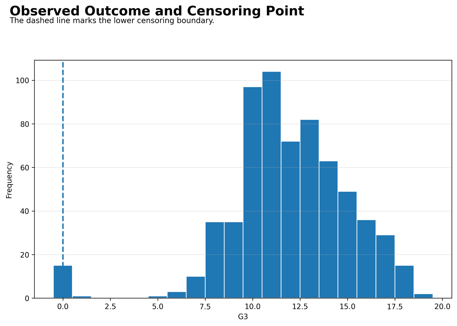
The distribution is centered in the low-to-mid teens, with a distinct stack of observations at the lower boundary of zero.
Fifteen of 649 observations are treated as censored, leaving 634 uncensored cases. G3 ranges from 0 to 19, with mean 11.9060 and median 12.
The spike at zero supplies the visual reason for considering Tobit Regression, but the small 2.311% censoring fraction means most information comes from exact positive grades.
The chart cannot determine whether zero is genuinely censored. That decision requires knowledge of how final grades were recorded.
Python Chart 2: Latent-Equation Coefficient Display
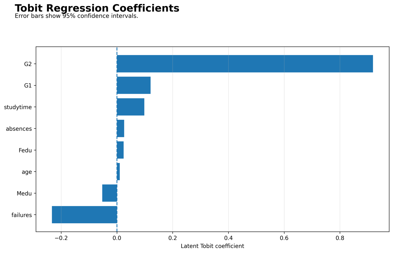
G2 has by far the longest positive bar; failures is the clearest negative coefficient; the remaining estimates cluster near zero.
G2 = 0.918706, G1 = 0.120714, studytime = 0.098237, and failures = −0.233112 on the latent scale.
The ranking describes conditional latent-mean associations within one eight-predictor Tobit Regression model.
The source coefficient table does not contain usable uncertainty estimates. Any apparent interval should not be interpreted as a valid 95% confidence interval until the covariance calculation is repaired.
Python Chart 3: Observed Values Versus Censor-Aware Predicted Means
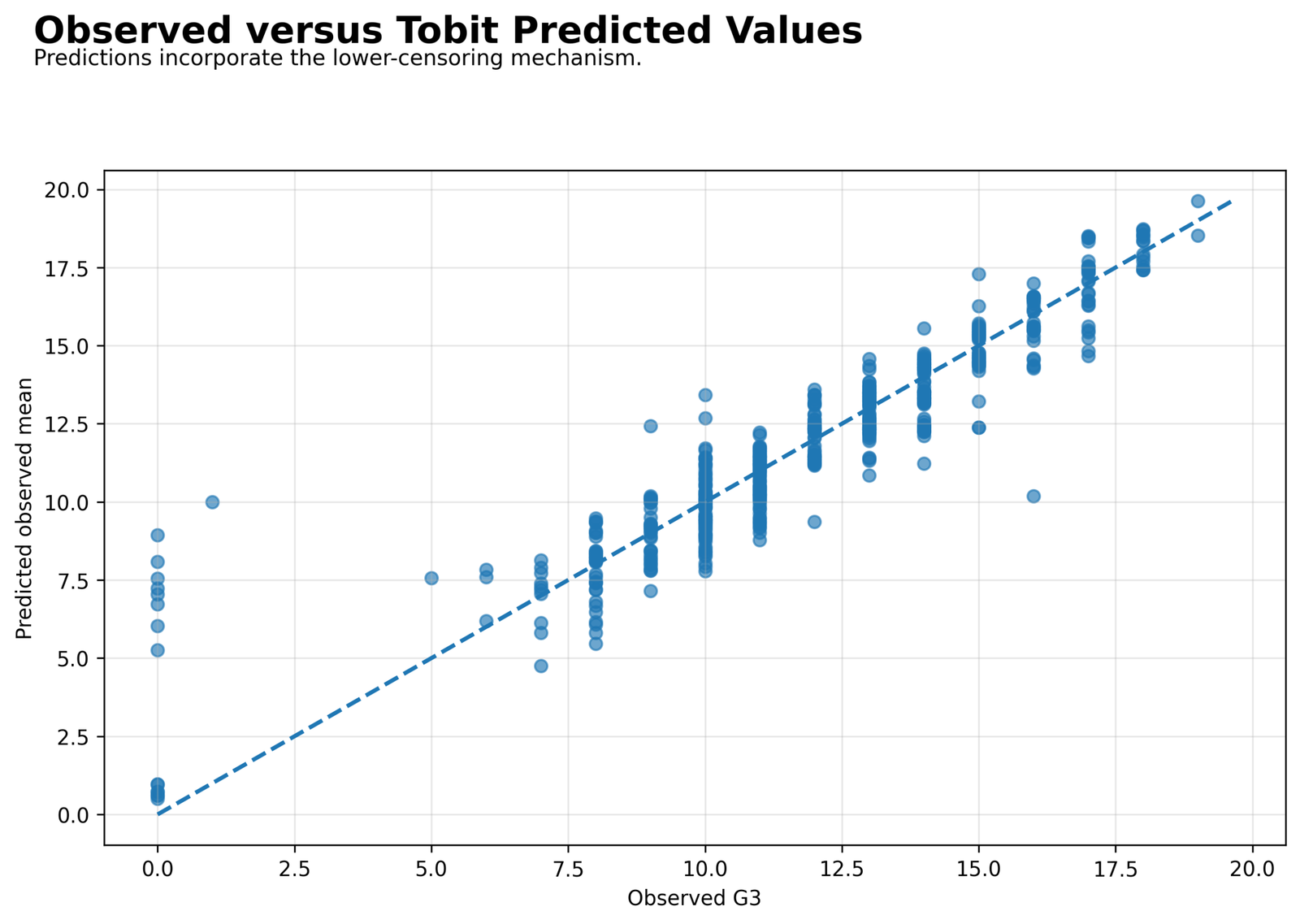
Most positive observations follow the diagonal trend, while the boundary observations form a separate lower cluster beneath their fitted means.
Observed-scale RMSE = 1.249837 and MAE = 0.790902 in the estimation sample.
The plotted predictions are expected observed means after integrating over the censoring rule, not simply the unbounded latent linear predictors.
The chart reveals overall fit and boundary errors, but in-sample agreement is not evidence of out-of-sample accuracy.
Python Chart 4: Observed Residuals Versus Predicted Values
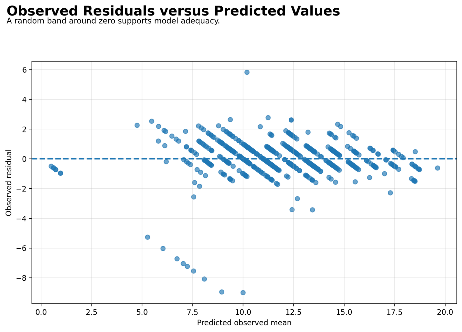
Residuals form diagonal bands because G3 takes integer values, and several cases show unusually large negative residuals.
The fitted sample has MAE 0.790902, yet a small set of low outcomes lies much farther below the model than the average error suggests.
The lower-tail discrepancies indicate that a single homoskedastic Gaussian latent equation may not describe every student equally well.
Residual structure should be investigated before treating model-level significance as evidence of adequate specification.
Python Chart 5: Latent Residual Distribution
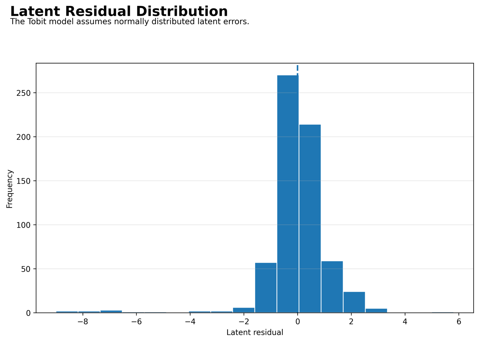
The distribution concentrates near zero but extends more strongly into the negative tail than into the positive tail.
The estimated latent residual scale is sigma = 1.271972, while several negative residuals are much larger in magnitude than that central scale.
Skewed or heavy-tailed latent residuals conflict with the standard Tobit Regression normal-error assumption.
The likelihood can converge even when its distributional assumptions are strained; the histogram therefore qualifies the inferential interpretation.
Python Chart 6: Normal Q-Q Plot of Latent Residuals
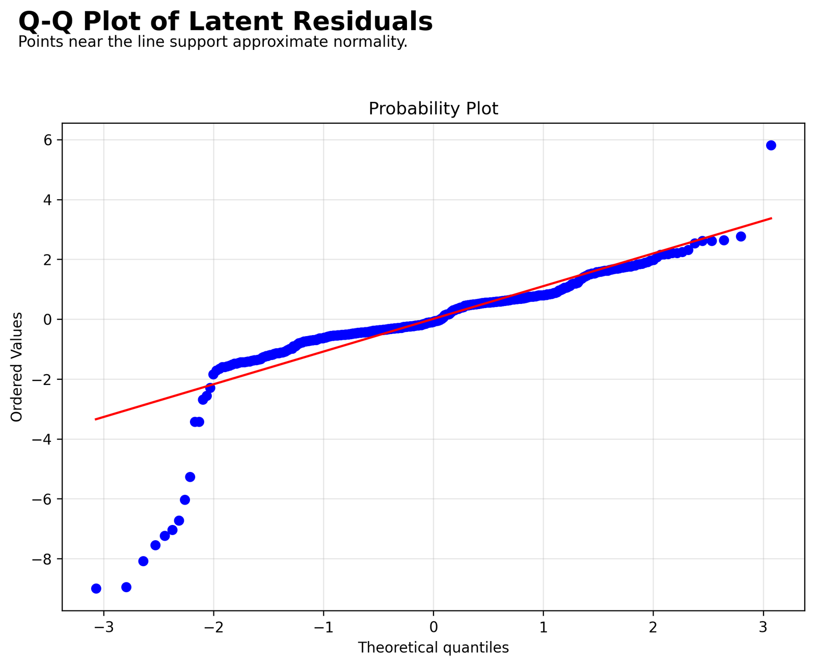
Middle quantiles approximately track the reference line, but the lower tail bends sharply away and the most positive residual also departs.
The strongest deviation occurs in the lower tail, consistent with boundary and low-grade cases that are poorly represented by the fitted Gaussian shape.
The Q-Q pattern does not support an unqualified normal latent-error claim.
Standard errors, likelihood tests, and marginal effects can be sensitive to error-distribution misspecification, so robust or alternative models deserve consideration.
Python Chart 7: Approximate Marginal Effects on the Observed Mean
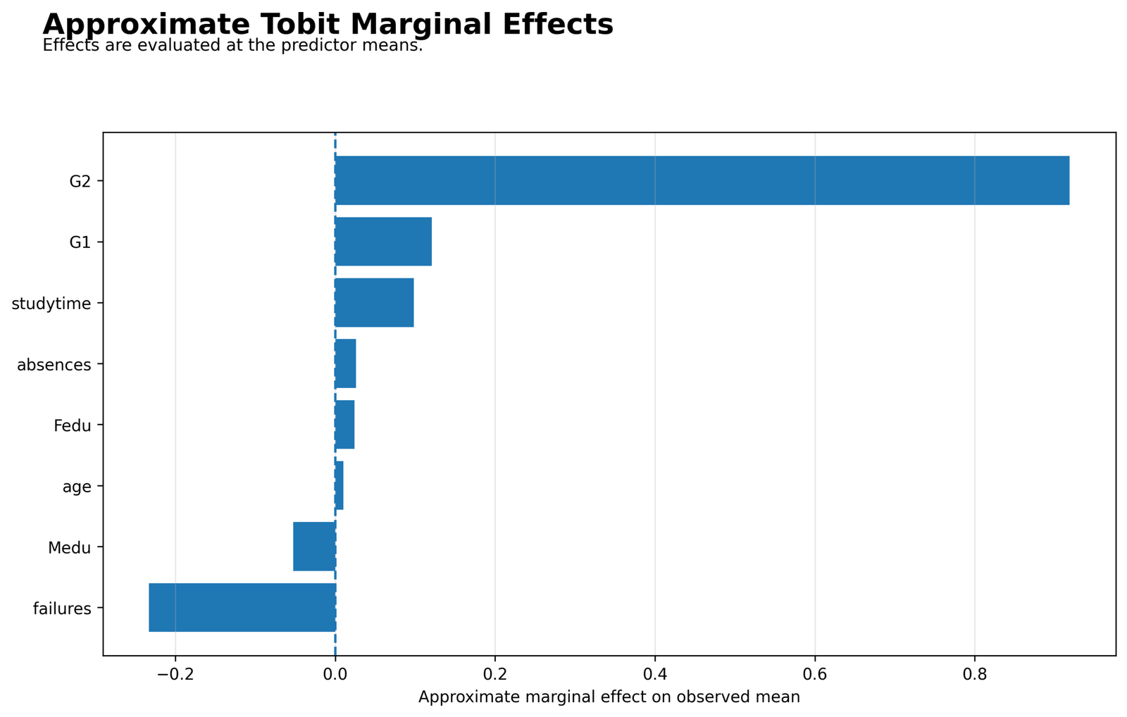
The ordering mirrors the latent coefficients because the estimated uncensoring probability at the predictor means rounds to one.
At the means, G2 = 0.918706, G1 = 0.120714, and failures = −0.233112 for both the latent slope and the approximate observed-mean effect.
The equality occurs because βj is multiplied by P(y > 0 | x), which is approximately 1.000 at that profile.
Marginal effects must be evaluated at a stated profile or averaged across cases. The displayed values are local effects at the predictor means, not universal constants.
Python Chart 8: Predicted Censoring Probability Distribution
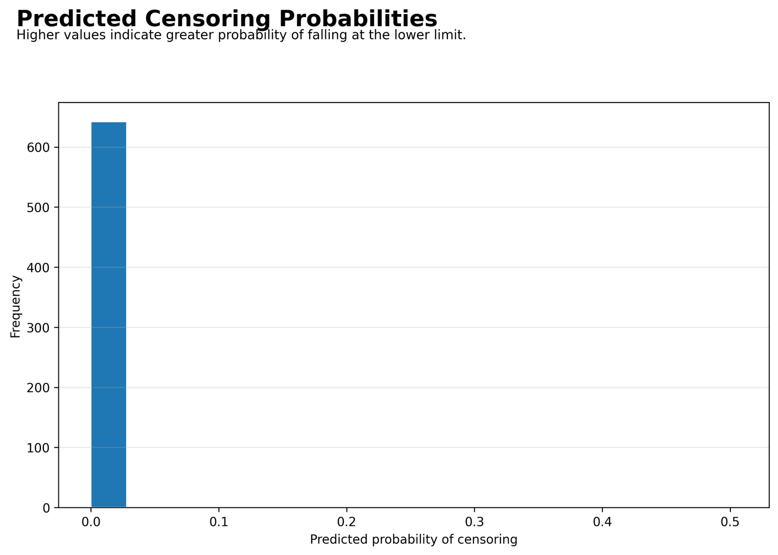
Most fitted censoring probabilities lie extremely close to zero, with only a small number of cases receiving meaningful boundary risk.
The dataset contains 15 observed boundary cases, while the mean-profile uncensoring probability rounds to 1.000.
The latent equation places most students far above the zero limit relative to sigma = 1.271972.
This pattern explains why the Tobit Regression fit resembles ordinary least squares and why the model has limited information about the latent region below zero.
Python Chart 9: Tobit Regression and OLS Information Criteria
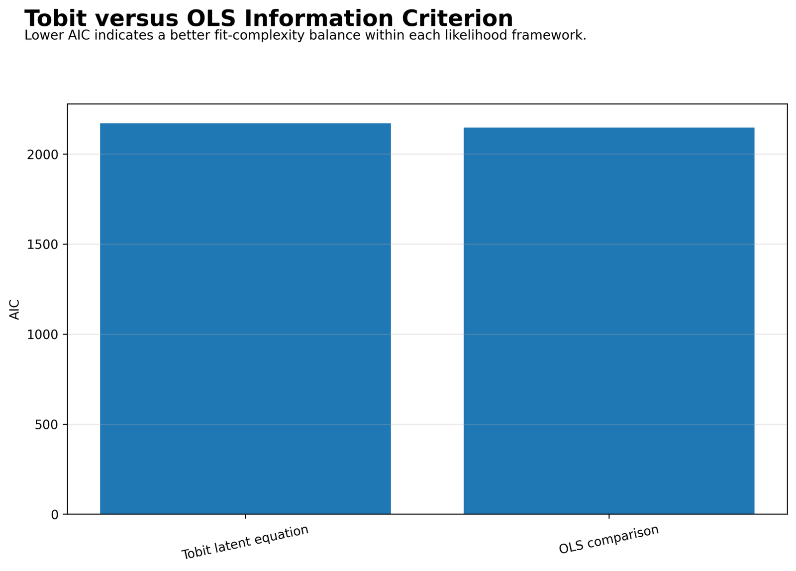
The OLS comparison has lower AIC and BIC than the fitted censored model in the supplied table.
Tobit AIC = 2170.6042 and BIC = 2215.3585; OLS AIC = 2146.3247 and BIC = 2186.6036.
With only 2.311% of responses at the limit, an ordinary linear fit closely approximates the observed data.
Model choice cannot rely on the smaller information criterion alone when the likelihoods encode different observation assumptions. The substantive status of zero remains decisive.
Python Chart 10: Tobit Regression Summary Table
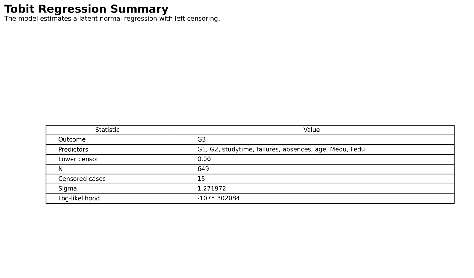
The compact panel gathers the outcome, predictor count, censoring rule, sample size, likelihood, sigma, and fit statistics.
N = 649, censored = 15, uncensored = 634, log likelihood = −1075.3021, LR χ²(8) = 1217.5713, and sigma = 1.2720.
The image is a visual index to the machine-readable tables rather than a replacement for coefficient, prediction, and diagnostic outputs.
A complete report should pair the summary with the censoring definition, effect scale, uncertainty limitation, and residual evidence.
Tobit Regression Coefficients and Marginal Effects
Tobit Regression coefficients live on the latent scale. They answer how the unobserved continuous response y* changes, not directly how the recorded boundary-adjusted mean changes. Observed-scale effects depend on the predicted probability that a case is uncensored.
Latent Coefficients
Holding all other predictors fixed, a one-unit increase in G2 is associated with a 0.918706-unit increase in the latent conditional mean of G3. A one-unit increase in G1 is associated with a 0.120714-unit increase. One additional prior failure is associated with a 0.233112-unit decrease. These are conditional associations, not causal effects.
Observed-Mean Marginal Effects at Predictor Means
| Predictor | Latent coefficient | P(uncensored) at means | Approx. observed-mean effect |
|---|---|---|---|
| G1 | 0.120714 | 1.000 | 0.120714 |
| G2 | 0.918706 | 1.000 | 0.918706 |
| studytime | 0.098237 | 1.000 | 0.098237 |
| failures | −0.233112 | 1.000 | −0.233112 |
| absences | 0.026001 | 1.000 | 0.026001 |
| age | 0.010276 | 1.000 | 0.010276 |
| Medu | −0.052647 | 1.000 | −0.052647 |
| Fedu | 0.024210 | 1.000 | 0.024210 |
The reported uncensoring probability at the vector of predictor means rounds to 1.000. Therefore each local observed-mean effect equals its latent coefficient at the displayed precision. For profiles closer to zero, the multiplier would be smaller and the observed-mean effect would be attenuated relative to the latent slope.
Three Effects That Should Not Be Confused
Predictions, Effects and Model Meaning
The worked prediction output contains four distinct quantities: the latent linear predictor μ, the predicted probability of censoring, the expected observed mean after applying the boundary, and the residual based on that observed mean. These quantities answer different questions and should remain in separate columns.
Prediction quantities
- Latent prediction: x′β, which may fall outside the observed range.
- Censoring probability: Φ[(c − μ)/σ].
- Expected observed mean: cΦ(z) + μ[1 − Φ(z)] + σφ(z).
- Boundary classification: a probability-based decision that should not be confused with the expected value.
Prediction limitations
- RMSE and MAE are calculated on the estimation sample.
- No train-test split or cross-validation is reported.
- The small censored group limits evaluation of boundary predictions.
- The model does not enforce a possible upper grade ceiling unless a right limit is added.
Tobit Regression produces smooth expected values, while G3 is recorded in integers. Diagonal residual bands are therefore expected. Large negative residuals are more important than the banding itself because they reveal cases whose observed outcomes are much lower than the latent equation predicts.
Tobit Regression Assumptions and Diagnostics
Standard Tobit Regression requires more than optimizer convergence. The observation rule, functional form, error distribution, variance structure, independence, and influential cases all affect the validity of coefficients and marginal effects.
Core assumptions
- The censoring limit is known and correctly classified.
- The latent conditional mean is linear in the specified predictors.
- Latent errors are normally distributed.
- Latent variance is constant across predictor profiles.
- Observations are independent or dependence is modeled.
- The same latent process governs censoring and positive magnitude.
Evidence in this analysis
- The lower limit is set to zero by the fitted specification.
- Only 15 observations are treated as censored.
- The residual histogram and Q-Q plot show lower-tail departures.
- Several large negative residuals warrant case review.
- No out-of-sample validation is available.
- Coefficient covariance recovery was unsuccessful.
Normality and Homoskedasticity
The latent residual histogram and Q-Q plot challenge a simple Gaussian error description, especially in the lower tail. The residual-versus-predicted plot also deserves scrutiny for changing spread and structure. Because standard Tobit Regression links the likelihood and marginal effects to both normality and common sigma, these are substantive model checks rather than cosmetic diagnostics.
Influence and Boundary Cases
With only 15 censored observations, a few boundary cases can have disproportionate influence on the fitted lower-tail mechanism. Case-deletion refits, score contributions, leverage-style summaries, and bootstrap stability checks would show whether the latent coefficients or sigma depend strongly on a small subset of students.
Upper-Bound Consideration
The fitted model uses a lower limit only. If the grade scale has an active upper ceiling, a two-limit Tobit Regression specification may be more appropriate. No observation in the supplied summary reaches 20, but the scientific design—not merely the sample maximum—should determine whether an upper censoring rule belongs in the model.
Tobit Regression in Python, R, SPSS and Excel
Cross-software agreement is meaningful only when every implementation uses the same 649 rows, lower limit, predictor coding, intercept, likelihood definition, optimization tolerance, and prediction formula. The supplied Python output is the primary numerical source for the worked results. R, SPSS, and Excel should be used to reproduce or audit the same specification rather than to fill missing inferential cells by substitution.
Python
Directly maximizes the censored normal likelihood, exports coefficients and sigma, and calculates latent predictions, censoring probabilities, observed means, residuals, charts, and fit statistics.
R
A censored-regression package can reproduce a left-censored Type I Tobit model. The dataset, left limit, formula, and case selection must exactly match the Python analysis before comparing estimates.
SPSS
Base linear regression is not a Tobit estimator. A censored-regression extension or Python integration must implement the censored likelihood. SPSS output should be checked for the same boundary and latent-scale interpretation.
Excel
The workbook is best used to audit μ, z, normal CDF and density terms, expected observed means, and residuals. Solver can illustrate likelihood maximization, but production uncertainty estimation is better handled in statistical software.
Code: Expand Only the Software You Need
These blocks show the essential Tobit Regression computation without reproducing the entire output-generation scripts.
Python: left-censored likelihood and expected observed mean
import numpy as np
from scipy import optimize, stats

def neg_loglik(theta, X, y, lower=0.0):
    beta = theta[:-1]
    sigma = np.exp(theta[-1])
    mu = X @ beta
    cens = y <= lower
    ll = np.empty_like(y, dtype=float)
    ll[~cens] = stats.norm.logpdf((y[~cens] - mu[~cens]) / sigma) - np.log(sigma)
    ll[cens] = stats.norm.logcdf((lower - mu[cens]) / sigma)
    return -ll.sum()

# X must include an intercept column.
# Start values can come from OLS; log(sigma) keeps sigma positive.
result = optimize.minimize(neg_loglik, start, args=(X, y, 0.0), method="BFGS")
beta = result.x[:-1]
sigma = np.exp(result.x[-1])

mu = X @ beta
z = (0.0 - mu) / sigma
p_censored = stats.norm.cdf(z)
expected_observed = mu * (1 - p_censored) + sigma * stats.norm.pdf(z)
R: Type I Tobit Regression
library(censReg)

fit <- censReg(
  G3 ~ G1 + G2 + studytime + failures + absences + age + Medu + Fedu,
  left = 0,
  right = Inf,
  data = dat
)

summary(fit)

# Observed-mean effect for predictor j at profile x:
# beta_j * pnorm((mu - left_limit) / sigma)
SPSS: specification and verification boundary
* Prepare the identical complete-case dataset and verify the limit.
DESCRIPTIVES VARIABLES=G3 G1 G2 studytime failures absences age Medu Fedu.
FREQUENCIES VARIABLES=G3.

* Base REGRESSION fits OLS, not Tobit.
* Use the installed censored-regression extension or Python integration
* that maximizes the same left-censored normal likelihood at c = 0.
* Verify N=649, censored=15, the coefficient vector, sigma,
* and log likelihood before interpreting the output.
Excel: row-level prediction formulas
Latent mean (mu):
=Intercept + SUMPRODUCT(Predictor_Row, Coefficient_Row)

z:
=(Lower_Limit - mu) / Sigma

P(censored):
=NORM.S.DIST(z, TRUE)

Expected observed mean:
=Lower_Limit*NORM.S.DIST(z,TRUE)
 +mu*(1-NORM.S.DIST(z,TRUE))
 +Sigma*NORM.S.DIST(z,FALSE)

Observed residual:
=Observed_G3 - Expected_Observed_Mean
Advanced Tobit Regression Topics
These 26 panels extend the worked analysis from basic interpretation to specification, uncertainty, alternatives, and reproducibility.
Tobit Regression Advanced Topic 1. Tobit Regression Type I Model
The classical Type I Tobit Regression model uses one latent normal equation and one deterministic censoring rule. The same coefficient vector determines both the latent mean and, through its distance from the limit, the probability of being censored. This economy is useful when the observation mechanism is genuinely a measurement or reporting limit. It becomes restrictive when a boundary value is generated by a separate behavioral decision. In the worked grade model, the assumption means G1, G2, studytime, failures, absences, age, Medu, and Fedu all influence the latent grade and the chance of appearing at zero through the same linear index. A researcher should defend that common-process assumption rather than treating it as a default created by software.
Tobit Regression Advanced Topic 2. Censoring Versus Truncation
Tobit Regression retains censored cases at the boundary. Truncated regression analyzes a sample from which cases beyond the threshold are absent. The distinction changes the likelihood: a censored case contributes a cumulative probability, while a truncated density is normalized by the probability of entering the observed region. Confusing the two can bias slopes and scale because the model uses the wrong information about missing or boundary observations. In the worked analysis, all 649 records remain present and 15 are treated as boundary values. That is a censoring specification. If students with latent grades below zero had been omitted entirely, the appropriate likelihood would be truncated rather than censored.
Tobit Regression Advanced Topic 3. Left, Right, and Two-Limit Tobit Regression
The worked model is left-censored at zero. Right-censored Tobit Regression is used when values above an upper limit are recorded at that ceiling. A two-limit model handles both lower and upper censoring. The model form must follow the data-collection rule. A grade scale may have both a floor and a ceiling even when the current sample does not contain observations at the upper endpoint. If the upper limit is an active reporting mechanism, a one-sided specification is incomplete. If no values are compressed at the ceiling, adding a right limit can be unnecessary. The correct choice depends on design knowledge, not only the observed minimum and maximum.
Tobit Regression Advanced Topic 4. Latent-Scale Interpretation
A Tobit Regression coefficient is a partial slope for the latent response y*. G2 = 0.918706 means that, conditional on the other seven predictors, a one-unit increase in G2 is associated with a 0.918706-unit increase in the latent mean. It does not automatically mean the recorded G3 rises by exactly that amount. Near the censoring limit, some latent movement changes the probability of escaping the boundary rather than appearing entirely as movement in the observed mean. Far from the limit, the observed and latent effects become similar. Stating the latent scale prevents a common reporting error and makes the later marginal-effect calculation transparent.
Tobit Regression Advanced Topic 5. Observed-Mean Marginal Effects
For a standard left-censored normal model, the derivative of the unconditional expected observed outcome is βj multiplied by the probability of being uncensored at the evaluation profile. This probability varies across cases, so an observed-mean marginal effect is generally not constant even though the latent coefficient is constant. The worked table evaluates effects at the vector of predictor means, where the uncensoring probability rounds to 1.000. That makes the displayed observed-mean effects numerically equal to the latent slopes. Average marginal effects would instead calculate the derivative for each of the 649 rows and then average those values. The two summaries should be labeled separately.
Tobit Regression Advanced Topic 6. Effect on the Probability of Being Uncensored
A predictor can also be interpreted through its effect on P(y > c | x). For a left-censored normal model, the derivative is βj φ((μ − c)/σ)/σ. The effect is largest for profiles near the limit, where the normal density is high, and becomes small when a case is already far above or below the boundary. Because most fitted profiles in this analysis have negligible censoring probability, the probability effects will be small for many students even when the latent G2 coefficient is large. This is another reason that one Tobit Regression coefficient cannot stand in for every substantive effect.
Tobit Regression Advanced Topic 7. Conditional Mean Among Uncensored Cases
A third target is E(y | y > c, x), the expected outcome among observations that are uncensored. Its derivative differs from both the latent coefficient and the unconditional observed-mean effect because conditioning changes the distribution through an inverse-Mills-ratio term. Analysts sometimes call every post-estimation derivative a “marginal effect” without naming the target. That practice creates conflicting numbers that are all mathematically valid but answer different questions. A clear Tobit Regression report should define the target population and scale before presenting any derivative.
Tobit Regression Advanced Topic 8. Small Censoring Fraction
Only 2.311% of the worked sample is treated as censored. A small censoring fraction often makes Tobit Regression resemble ordinary least squares because most rows contribute ordinary normal-density terms. It also means the lower-tail mechanism is estimated from limited direct information. The model may be sensitive to a few boundary cases, and complex heteroskedastic or nonlinear censoring behavior can be difficult to identify. Small censoring does not make the method wrong when the observation rule is real, but it reduces the practical difference from OLS and increases the importance of sensitivity analysis.
Tobit Regression Advanced Topic 9. Tobit Regression Versus OLS
The OLS comparison has slightly lower in-sample RMSE and MAE and lower displayed AIC and BIC. That result is unsurprising with only 15 boundary cases. However, OLS and Tobit Regression encode different meanings for zero. OLS treats it as exact; Tobit treats it as incomplete information about an underlying value. Predictive error cannot by itself decide which scientific statement is correct. A defensible comparison therefore combines fit, residual evidence, boundary calibration, and the substantive recording mechanism. When zero is exact, OLS or another bounded-outcome model may be preferable. When zero is censored, the Tobit likelihood respects the observation rule even if its in-sample RMSE is not smaller.
Tobit Regression Advanced Topic 10. Information-Criterion Caveat
AIC and BIC compare penalized likelihoods, but meaningful comparison requires compatible response definitions, observation sets, and likelihood constants. The attached table places Tobit Regression and OLS criteria side by side. The lower OLS values are informative as a descriptive comparison, yet they do not prove that censoring should be ignored. If the two models treat boundary observations as different kinds of information, the scientific interpretation still matters. Information criteria help select among defensible candidates; they do not validate an indefensible observation mechanism.
Tobit Regression Advanced Topic 11. Normal Latent Errors
Standard Tobit Regression assumes normal latent errors. The Q-Q plot shows strong lower-tail departure, and the histogram is asymmetric. These patterns can affect maximum-likelihood estimates and especially their uncertainty. A few extreme low outcomes may create more probability mass in the tail than a Gaussian model allows. Possible responses include robust sensitivity checks, alternative latent distributions, censored quantile methods, or explicit mixture structures. The correct reaction is not to discard the model automatically, but to report the departure and test whether substantive conclusions persist under reasonable alternatives.
Tobit Regression Advanced Topic 12. Homoskedasticity
The classical model uses one sigma for every predictor profile. If latent variance changes with grade history, studytime, failures, or another covariate, both the probability of censoring and the expected observed outcome can be misspecified. Residual-versus-fitted plots may reveal changing spread, but formal heteroskedastic Tobit Regression lets log sigma depend on predictors. Such flexibility increases complexity and requires enough boundary information. With only 15 censored cases, a richly parameterized variance equation could be unstable. Parsimony and sensitivity analysis are therefore important.
Tobit Regression Advanced Topic 13. Heteroskedastic Tobit Regression
A heteroskedastic specification replaces constant sigma with a positive function such as exp(z′γ). This can separate changes in the latent mean from changes in latent dispersion. It is useful when residual spread clearly varies across groups or predictor levels. Interpretation becomes more complex because a predictor in the scale equation changes censoring probabilities and observed means even when it is absent from the mean equation. The worked output does not estimate a scale equation, so heteroskedastic effects should be described as a possible extension rather than a result.
Tobit Regression Advanced Topic 14. Nonlinearity and Transformations
The worked Tobit Regression enters every predictor linearly. Grade relationships may contain diminishing returns, thresholds, or ceiling effects. Residual curvature, partial-residual plots for uncensored cases, and substantive theory can motivate polynomial terms, splines, or transformations. Any nonlinear term affects the latent mean and therefore the censoring probability. Marginal effects then depend on both the nonlinear derivative and the uncensoring probability. A better functional form can matter more than choosing between OLS and Tobit when the linear predictor is misspecified.
Tobit Regression Advanced Topic 15. Interactions
An interaction allows the latent effect of one predictor to depend on another. For example, the relationship between G2 and final grade might differ by prior failures or studytime. In Tobit Regression, an interaction coefficient is not the complete observed-scale interaction effect because censoring introduces additional nonlinearity. Researchers should compute predicted observed means or marginal effects across meaningful combinations rather than interpreting the product-term coefficient alone. No interactions are included in the worked model, so the reported slopes are average additive associations.
Tobit Regression Advanced Topic 16. Multicollinearity
Tobit Regression does not solve predictor overlap. G1 and G2 are earlier grades and are likely to share substantial information. Multicollinearity can inflate uncertainty, destabilize signs, and make one coefficient appear small after another correlated predictor enters. The dominance of G2 should therefore be interpreted within the chosen eight-predictor specification. VIF-style diagnostics from the corresponding design matrix, condition indices, and specification comparisons can help assess stability, even though the final estimator is maximum likelihood rather than OLS.
Tobit Regression Advanced Topic 17. Influential Boundary Observations
Boundary cases can contribute strongly to the cumulative-probability part of the likelihood. With only 15 censored observations, one unusual predictor profile may noticeably affect beta or sigma. Case-deletion refits, likelihood-contribution plots, and bootstrap inclusion frequencies can identify that dependence. Influence should be assessed on coefficients, marginal effects, and predicted censoring probabilities. Removing a difficult case solely to improve diagnostics is not justified; the goal is to understand sensitivity and possible data-quality problems.
Tobit Regression Advanced Topic 18. Bootstrap Uncertainty
When the numerical Hessian is unreliable, a case-resampling bootstrap can estimate empirical uncertainty. Each bootstrap sample should resample complete records, refit the entire Tobit Regression model, and recompute the target coefficients or marginal effects. Failed or boundary solutions must be tracked rather than silently discarded. Percentile or bias-corrected intervals can then be reported with the number of successful refits. The attached analysis contains no bootstrap results, so no such intervals are claimed. Bootstrap uncertainty is an extension that could repair the current inferential gap.
Tobit Regression Advanced Topic 19. Hessian and Covariance Failure
Successful optimization means the algorithm found a parameter vector that satisfied its convergence criteria. It does not guarantee that the inverse Hessian is accurate or positive definite. Flat curvature, scaling problems, strong predictor overlap, or numerical approximation can prevent covariance recovery. The attached output preserves blank standard errors rather than converting failed calculations into zeros or nonsignificant tests. A careful workflow would rescale predictors, compare optimizers, calculate a more stable numerical Hessian, use profile likelihood, or bootstrap the estimates.
Tobit Regression Advanced Topic 20. Alternative Models for Exact Zeros
If G3 = 0 is an exact earned grade, standard Tobit Regression may impose a false latent-below-zero story. Ordinary regression with robust uncertainty, ordinal regression, bounded regression, or a model tailored to the grade-generating process may be more defensible. If zeros arise from a separate event such as nonparticipation, a two-part model can estimate the zero process separately from positive grades. The presence of zeros is a diagnostic clue, not a model-selection command.
Tobit Regression Advanced Topic 21. Two-Part and Cragg Models
A two-part model first estimates the probability of being above the boundary and then models the positive outcome among uncensored cases. Predictor effects may differ across parts. This flexibility is useful when crossing the boundary and determining positive magnitude are substantively distinct processes. The cost is additional parameters and a different estimand. Tobit Regression is more restrictive because one latent equation governs both pieces. Comparing the models can reveal whether the common-process assumption is plausible.
Tobit Regression Advanced Topic 22. Censored Quantile Regression
Censored quantile regression targets a conditional quantile of the latent or observed response rather than the conditional mean under normal errors. It can reveal whether predictor effects differ across the outcome distribution and may be more robust to heavy tails. Interpretation and estimation differ from the Tobit likelihood, and standard errors often rely on resampling. The strong lower-tail departure in the worked diagnostics makes quantile-based sensitivity analysis especially relevant, although no censored quantile results are available here.
Tobit Regression Advanced Topic 23. Sample Selection Is Not Tobit Censoring
A Heckman-style selection problem occurs when the outcome is observed only for a nonrandom subset and the selection mechanism has an unobserved component correlated with the outcome error. Tobit censoring instead assumes the outcome is transformed by a known limit. Both use latent-variable ideas and normal probabilities, which encourages confusion. The correct method follows the data mechanism: boundary recording calls for censoring; nonrandom missing outcomes call for a selection model. The 649-case worked dataset retains all records, so the fitted specification is censoring rather than sample selection.
Tobit Regression Advanced Topic 24. Out-of-Sample Validation
The reported RMSE and MAE are in-sample summaries. A predictive Tobit Regression application should use a holdout set, cross-validation, or temporal validation. Evaluation should include overall observed-scale error, calibration of censoring probabilities, error among uncensored cases, and performance for boundary cases. Because only 15 observations are censored, random folds may contain very few boundary cases; stratified or repeated resampling can stabilize evaluation. No external validation is available in the attached analysis.
Tobit Regression Advanced Topic 25. Communication and Reporting
A high-quality Tobit Regression report states the censoring limit, number and percentage censored, latent equation, scale parameter, likelihood statistic, coefficient scale, marginal-effect target, diagnostics, and uncertainty method. It should also explain why censoring is scientifically credible. Avoid phrases such as “a one-unit increase causes a 0.92-unit observed increase” unless a causal design and the correct observed-scale derivative justify that statement. Transparent limits strengthen rather than weaken the analysis.
Tobit Regression Advanced Topic 26. Reproducibility and Case-Level Audit
Reproducibility requires more than saving the final coefficient table. The same complete-case rows, variable coding, limit, optimizer settings, parameterization of sigma, and prediction equations must be preserved. A case-level ledger containing observed G3, latent μ, censoring probability, expected observed mean, and residual allows reviewers to trace charts and summary metrics. The downloadable Python report and worked workbook support that audit. A future R or SPSS reproduction should be reconciled against those quantities once the same specification is confirmed.
APA-Style Reporting for Tobit Regression
A concise report should distinguish model-level evidence from unavailable coefficient-level uncertainty. One defensible wording is:
For a journal or thesis, add the full formula, exact coding, censoring justification, software and version, optimization method, marginal-effect definition, and sensitivity analyses. Round displayed statistics consistently while retaining full precision in downloadable tables.
Tobit Regression Publication Checklist
Before fitting
- Verify that boundary values are censored rather than exact.
- Identify left, right, or two-limit censoring.
- Define the latent outcome and predictor coding.
- Check missingness, range, and duplicate records.
- Plan alternative models for sensitivity analysis.
Before publication
- Report N and the censored count and percentage.
- Name the latent and observed effect scales.
- Include sigma, likelihood, AIC, BIC, and diagnostics.
- Do not invent missing standard errors or p-values.
- Separate in-sample fit from predictive validation.
- State that observational coefficients are not causal.
Tobit Regression Downloads and Chart Resources
The files below support verification of the worked Tobit Regression results, calculations, and software output.
Quick report downloads
Open the main reports and workbook directly.
Frequently Asked Questions About Tobit Regression
Tobit Regression FAQ: What is Tobit Regression?
Tobit Regression is a maximum-likelihood model for a continuous latent outcome that is censored at one or more known limits. It combines exact-density contributions for uncensored observations with cumulative-probability contributions for censored observations.
Tobit Regression FAQ: Is Tobit Regression appropriate whenever an outcome contains zeros?
No. Zeros must represent censoring at a known limit rather than exact valid outcomes or a separate participation process. A hurdle, two-part, ordinal, count, or ordinary regression model may be more appropriate for other zero-generating mechanisms.
Tobit Regression FAQ: What is the difference between censoring and truncation?
Censored cases remain in the dataset at a boundary, while truncated cases are absent from the observed sample. The two mechanisms require different likelihoods.
Tobit Regression FAQ: What does a Tobit Regression coefficient mean?
It is the change in the latent conditional mean associated with a one-unit predictor increase, holding other variables fixed. It is not automatically the change in the expected observed outcome.
Tobit Regression FAQ: How do I obtain an observed-mean marginal effect?
For a standard left-censored normal model, multiply the latent coefficient by the predicted probability of being uncensored at the evaluation profile. Average marginal effects repeat this calculation for every case and average the results.
Tobit Regression FAQ: Why do the worked marginal effects equal the coefficients?
At the vector of predictor means, the predicted uncensoring probability rounds to 1.000. Multiplying each latent coefficient by that value produces the same displayed number.
Tobit Regression FAQ: How many observations are censored in the worked example?
The model treats 15 of 649 observations as left-censored at zero, which is 2.311% of the analysis sample.
Tobit Regression FAQ: Is the Tobit Regression model statistically significant?
The eight predictors are jointly informative according to LR χ²(8) = 1217.57, p < .001. This global test does not establish significance for each individual coefficient.
Tobit Regression FAQ: Which predictor is strongest in the worked model?
G2 has the largest positive latent coefficient, b = 0.918706, after adjustment for the other seven predictors.
Tobit Regression FAQ: Can I report p-values for the individual coefficients?
Not from the supplied coefficient table. Standard errors, z values, p-values, and confidence intervals were not recovered, so coefficient-level significance should not be invented.
Tobit Regression FAQ: What does sigma mean in Tobit Regression?
Sigma is the standard deviation of the latent normal error distribution. The worked estimate is 1.271972.
Tobit Regression FAQ: Why compare Tobit Regression with OLS?
OLS provides a useful sensitivity comparison because the censoring fraction is small. The methods differ in how they interpret boundary values, so fit statistics must be considered alongside the observation mechanism.
Tobit Regression FAQ: Do lower AIC and BIC for OLS prove OLS is correct?
No. Information criteria help compare defensible likelihood models, but they cannot determine whether zero is scientifically censored or exact.
Tobit Regression FAQ: What diagnostics are most important?
Check the censoring inventory, observed-versus-predicted values, residuals versus fitted values, latent residual distribution, Q-Q plot, influential cases, and censoring-probability calibration.
Tobit Regression FAQ: Can Tobit Regression handle both lower and upper limits?
Yes. A two-limit Tobit model can represent active lower and upper censoring. The worked model uses only a lower limit of zero.
Tobit Regression FAQ: Is Tobit Regression causal?
No. The worked model describes adjusted associations in observational data. Causal interpretation requires a design and assumptions that address confounding, selection, and intervention meaning.
Tobit Regression Conclusion
Tobit Regression is valuable when a continuous latent response is observed through a genuine censoring rule. In the worked 649-case analysis, 15 G3 values are treated as left-censored at zero. The eight-predictor model is strongly supported at the global level, G2 has the largest positive latent coefficient, failures has a negative coefficient, and the local observed-mean effects at predictor means match the latent slopes because the estimated uncensoring probability rounds to one.
The analysis also shows why responsible reporting goes beyond a significant likelihood-ratio test. The censoring status of zero must be justified, the lower-tail residuals challenge normality, only a small fraction of cases informs the censoring mechanism, coefficient uncertainty is unavailable, and the reported prediction errors are in-sample. The correct conclusion is therefore a strong joint latent association with explicit diagnostic and inferential reservations—not a causal or universally transferable grade equation.

