
McNemar Bowker Test: Formula, Interpretation, Calculator, Python, R, SPSS and Excel Guide
McNemar Bowker Test extends McNemar's paired binary test to a square table with more than two categories. This complete guide explains the symmetry hypothesis, formula, informative-pair degrees of freedom, worked 4 × 4 transition table, calculator workflow, APA reporting, six paired Python and R chart stories, SPSS and Excel workflows, code and downloadable reports through a verified G2-to-G3 grade-band analysis of 649 students.
649 paired observations
Bowker χ² = 76.2816
Verified p = 1.92 × 10⁻¹⁶
McNemar Bowker Test Model Overview
McNemar Bowker Test, also called Bowker's test of symmetry or the McNemar–Bowker extension, evaluates whether paired transitions between every pair of categories are directionally balanced. The same 649 students are classified into four G2 grade bands and again into four G3 grade bands. The test compares each off-diagonal cell with its mirror cell across the main diagonal.
What question does the McNemar Bowker Test answer?
The method asks whether movement from grade band i at G2 to grade band j at G3 occurs as often as movement from j at G2 to i at G3. In the current analysis, the question is whether the complete G2-to-G3 transition matrix is symmetric.
How it extends the ordinary McNemar test
The ordinary McNemar test applies to paired binary classifications and uses one discordant pair. The McNemar Bowker Test applies to a square k × k table and sums a McNemar-style contribution across every informative off-diagonal category pair. For four categories, there can be six possible pairs, although pairs with no transitions in either direction contribute nothing and provide no information.
Worked example at a glance
The observed transition table contains 521 students on the diagonal and 128 students who changed grade band. Upward band transitions total 113, while reverse-direction transitions total 15. The verified Bowker statistic is 76.2815729. Only three category pairs have nonzero discordant totals, so the verified analysis uses df = 3. The verified p-value is 1.9248733 × 10⁻¹⁶.
Quick Answer: McNemar Bowker Test Result
The McNemar Bowker Test rejects the null hypothesis of paired transition symmetry. The result is driven by three informative off-diagonal pairs, all showing substantially more upward than downward movement.
Test summary
- Procedure: McNemar Bowker Test of symmetry
- Design: paired four-category G2-to-G3 transition table
- Statistic: χ²B = 76.2815729
- Informative-pair df: 3
- Verified p-value: 1.9248733 × 10⁻¹⁶
- Decision at α = .05: reject H0
Substantive meaning
- Band 1→2 transitions: 56; reverse 2→1 transitions: 11.
- Band 2→3 transitions: 45; reverse 3→2 transitions: 3.
- Band 3→4 transitions: 12; reverse 4→3 transitions: 1.
- Net upward transitions exceed downward transitions by 98.
- The paired change pattern is not directionally balanced.
Table of Contents
- Research question, hypotheses and paired design
- When to use the McNemar Bowker Test
- McNemar Bowker Test formula and calculation
- Variables and data dictionary
- Worked 4 × 4 transition table and complete results
- McNemar Bowker versus related paired tests
- McNemar Bowker Test calculator workflow
- Six Python and R chart interpretations
- Python, R, SPSS and Excel workflows
- Expandable code for the McNemar Bowker Test
- Assumptions, limitations and advanced interpretation
- APA reporting for the McNemar Bowker Test
- Common McNemar Bowker Test mistakes
- Reports and worked Excel download
- Related Salar Cafe guides
- Frequently asked questions
- McNemar Bowker Test conclusion
Research Question, Hypotheses and Paired Design
Research question
Are G2-to-G3 movements between the four grade bands directionally symmetric, or do some transitions occur more often in one direction than in the reverse direction?
Null and alternative hypotheses
| Hypothesis | Statistical statement | Meaning |
|---|---|---|
| Null hypothesis | H0: pij = pji for all i < j | Every transition direction is balanced by its reverse direction. |
| Alternative hypothesis | H1: at least one pij ≠ pji | At least one pair of categories has directional imbalance. |
Why this is a paired design
Each row and column classification belongs to the same student. That dependence is essential. An ordinary chi-square test of independence would treat the row and column classifications as if they came from independent observations and would answer a different question. The McNemar Bowker Test uses the mirrored off-diagonal cells created by the paired design.
Grade-band coding used in the workbook
The workbook preserves the category coding as grade bands 1, 2, 3 and 4. Band 1 is the lowest category and band 4 is the highest. Therefore, cells above the main diagonal represent movement to a higher band, and cells below the diagonal represent movement to a lower band.
When to Use the McNemar Bowker Test
Use the McNemar Bowker Test when
- The same participants are classified twice.
- Both classifications use the same set of three or more nominal or ordered categories.
- The resulting table is square.
- The research question concerns directional symmetry of category changes.
- You want a multi-category extension of McNemar's paired binary test.
- Off-diagonal transition counts are the main inferential focus.
Choose another method when
- The two samples are independent rather than paired.
- The row and column variables use different category sets.
- The table is not square.
- You only need agreement strength; use a kappa statistic instead.
- You specifically need marginal homogeneity rather than full symmetry.
- Covariate adjustment or repeated multilevel structure is required.
Simple test-selection logic
If no, use an independent-sample contingency-table method.
If yes, use the ordinary McNemar test.
If yes, use the McNemar Bowker Test for symmetry.
Symmetry is stricter than marginal homogeneity
Full symmetry requires each mirrored cell pair to match. Marginal homogeneity concerns equality of the row and column marginal distributions. Symmetry implies marginal homogeneity, but marginal homogeneity does not necessarily require every individual mirrored pair to be equal.
For background on paired categorical tables and related methods, see Bowker's Test of Symmetry, cross-tabulation and two-way tables and relative frequency.
McNemar Bowker Test Formula and Calculation
The McNemar Bowker Test compares every upper-triangle off-diagonal count with its mirrored lower-triangle count. Each informative pair contributes a squared directional difference divided by the total discordant count for that pair.
Step 1: Identify the mirrored category pairs
With four categories, the possible pairs are 1↔2, 1↔3, 1↔4, 2↔3, 2↔4 and 3↔4. In this transition table, only 1↔2, 2↔3 and 3↔4 contain nonzero discordant totals.
Step 2: Calculate each pair contribution
| Pair | nij | nji | Difference | Pair total | Contribution |
|---|---|---|---|---|---|
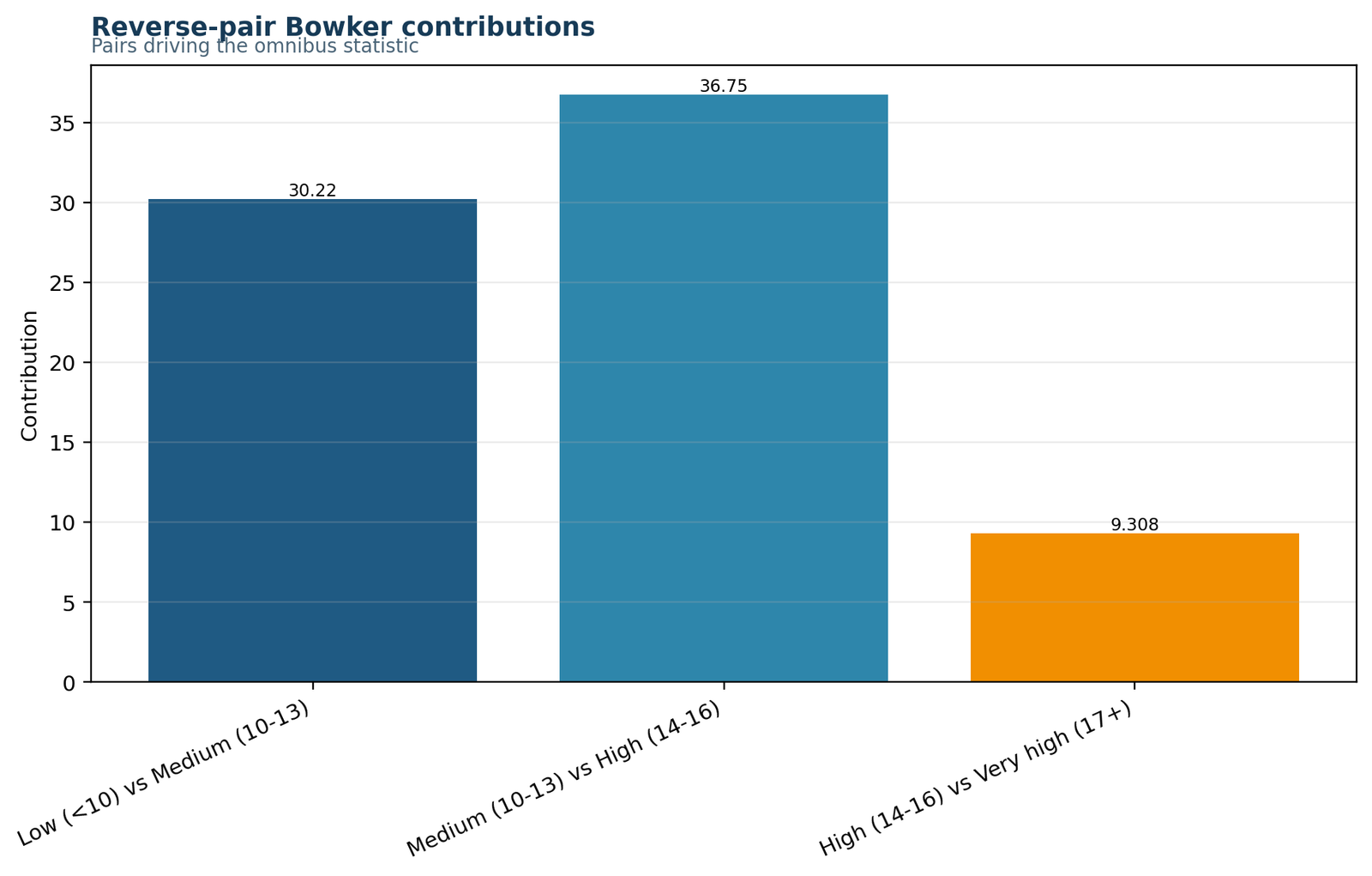
| 1 vs 2 | 56 | 11 | 45 | 67 | 30.2238806 |
| 1 vs 3 | 0 | 0 | 0 | 0 | 0 |
| 1 vs 4 | 0 | 0 | 0 | 0 | 0 |
| 2 vs 3 | 45 | 3 | 42 | 48 | 36.7500000 |
| 2 vs 4 | 0 | 0 | 0 | 0 | 0 |
| 3 vs 4 | 12 | 1 | 11 | 13 | 9.3076923 |
Step 3: Sum the contributions
Step 4: Determine the degrees of freedom
A four-category square table has a theoretical maximum of 4(4−1)/2 = 6 mirrored pairs. However, three pairs have zero discordant totals and add no information. The verified Python, R and SPSS-aligned analysis therefore uses the number of informative pairs, df = 3.
Step 5: Obtain the p-value
The verified reference p-value is 1.9248733079049484 × 10⁻¹⁶. The Excel formula display reaches the floating-point boundary at 2.220446049250313 × 10⁻¹⁶; the article uses the independently verified reference value.
Variables and Data Dictionary
| Variable | Role | Coding | N | Meaning in the analysis |
|---|---|---|---|---|
| G2 | Original first paired grade | Numeric grade values | 649 | Source variable for the first grade-band classification. |
| G2 grade band | Row classification | 1, 2, 3, 4 | 649 | Starting paired category. |
| G3 | Original second paired grade | Numeric final grade values | 649 | Source variable for the second grade-band classification. |
| G3 grade band | Column classification | 1, 2, 3, 4 | 649 | Ending paired category. |
Observed 4 × 4 transition table
| G2 band | G3 band 1 | G3 band 2 | G3 band 3 | G3 band 4 | Row total |
|---|---|---|---|---|---|
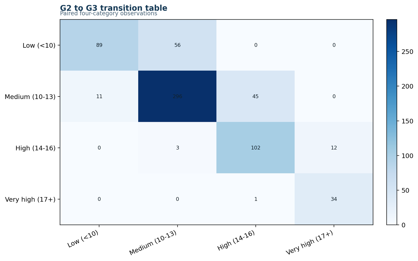
| 1 | 89 | 56 | 0 | 0 | 145 |
| 2 | 11 | 296 | 45 | 0 | 352 |
| 3 | 0 | 3 | 102 | 12 | 117 |
| 4 | 0 | 0 | 1 | 34 | 35 |
| Column total | 100 | 355 | 148 | 46 | 649 |
Diagonal and off-diagonal structure
| Structure | Count | Percent of N | Meaning |
|---|---|---|---|
| Unchanged diagonal classifications | 521 | 80.28% | Students remained in the same grade band. |
| All changed classifications | 128 | 19.72% | Students moved to a different band. |
| Upward transitions | 113 | 17.41% | G3 band was higher than G2 band. |
| Downward transitions | 15 | 2.31% | G3 band was lower than G2 band. |
Worked 4 × 4 Transition Table and Complete Results
80.28% on the main diagonal
19.72% off the diagonal
17.41% of all students
2.31% of all students
Three informative mirrored pairs
Reject symmetry decisively
Primary McNemar Bowker Test result
| Test | Statistic | df | Verified p-value | Decision at α = .05 |
|---|---|---|---|---|
| McNemar Bowker Test | 76.2815729 | 3 | 1.9248733 × 10⁻¹⁶ | Reject H0 |
Contribution shares
| Pair | Contribution | Share of total χ² | Directional interpretation |
|---|---|---|---|
| 1 vs 2 | 30.2239 | 39.62% | Substantially more 1→2 transitions than 2→1 transitions. |
| 2 vs 3 | 36.7500 | 48.18% | Largest contribution; strongly favors 2→3 movement. |
| 3 vs 4 | 9.3077 | 12.20% | More 3→4 transitions than 4→3 transitions. |
Marginal distribution change
The G2 marginal counts are 145, 352, 117 and 35, while the G3 marginal counts are 100, 355, 148 and 46. Band 1 decreases by 45 students, band 2 increases by 3, band 3 increases by 31 and band 4 increases by 11. These marginal changes align with the directional off-diagonal evidence.
Statistical and practical interpretation
The p-value is far below any conventional significance threshold, so the statistical conclusion is unambiguous. The substantive pattern is also clear: 113 students moved upward compared with only 15 moving downward. However, the McNemar Bowker Test does not itself provide a standardized effect-size measure. Report the transition counts, direction and percentages rather than inventing a generic effect size.
McNemar Bowker Test Versus Related Paired Tests
Paired binary test for one discordant category pair in a 2 × 2 table.
Paired multi-category symmetry test for a square k × k table.
Tests equality of paired marginal distributions rather than every mirrored cell pair.
Measures agreement beyond chance; it does not test directional transition symmetry.
| Method | Data design | Null question | Main output |
|---|---|---|---|
| McNemar test | Paired 2 × 2 | Are the two discordant counts equal? | One paired binary symmetry statistic. |
| McNemar Bowker Test | Paired k × k | Is every nij equal to nji? | Global symmetry statistic and pair contributions. |
| Stuart–Maxwell test | Paired k × k | Are row and column marginal distributions equal? | Marginal homogeneity statistic. |
| Kappa statistic | Paired ratings | How much agreement exceeds chance? | Agreement coefficient and confidence interval. |
Why the ordinary chi-square test is not a substitute
An ordinary chi-square test treats the two classifications as independent variables. The McNemar Bowker Test uses the paired nature of the table and evaluates mirrored transition counts. The tests answer different questions and use different reference structures.
Why high agreement can coexist with significant asymmetry
Agreement is determined largely by the diagonal, whereas symmetry is determined by the balance of off-diagonal pairs. In this analysis, 80.28% stayed in the same band, yet the remaining changes were overwhelmingly upward. Therefore, high diagonal agreement and strong directional asymmetry occur together.
For a separate agreement-focused analysis, see Cohen's Kappa. For the closely related symmetry method, see Bowker's Test of Symmetry.
McNemar Bowker Test Calculator: Step-by-Step Workflow
A reliable McNemar Bowker Test calculator must accept a square paired transition matrix, compare every mirrored off-diagonal pair, exclude zero-total pairs from informative degrees of freedom when that is the selected implementation, and return the global statistic together with pair-level contributions.
Calculator inputs for the worked example
| Input | Value | Meaning |
|---|---|---|
| Number of categories | 4 | Grade bands 1 through 4. |
| Row variable | G2 grade band | Starting paired classification. |
| Column variable | G3 grade band | Ending paired classification. |
| Total paired cases | 649 | Every student contributes one row-column pair. |
| Alpha | 0.05 | Prespecified decision threshold. |
Calculator step 1: verify the matrix is square
The row and column categories must match in number and meaning. A rectangular table cannot be evaluated with the standard McNemar Bowker symmetry formula.
Calculator step 2: inspect the diagonal and off-diagonal counts
The diagonal counts describe unchanged classifications. The inferential statistic uses only off-diagonal mirrored pairs. In the worked matrix, the diagonal sum is 521 and the off-diagonal sum is 128.
Calculator step 3: compare mirrored pairs
The calculator should display 56 versus 11, 45 versus 3 and 12 versus 1 as the three informative pairs. The three zero-versus-zero pairs should contribute zero.
Calculator step 4: confirm the statistic and df
The expected target is χ²B = 76.2815729 with 3 informative-pair degrees of freedom. A calculator that automatically reports df = 6 should be checked to determine how it handles zero-total pairs.
Calculator step 5: interpret the direction
The global p-value indicates whether symmetry fails, but pair directions explain how it fails. Here, all informative pairs show more upward than downward movement.
Six Python and R McNemar Bowker Test Chart Interpretations
The Python and R charts cover the same paired transition structure from complementary visual angles. Each chart pair is interpreted once through Pattern, Key Values, Interpretation, Why It Matters and Next Step.
Chart pair 1: Transition table and transition matrix
Most observations lie on the diagonal
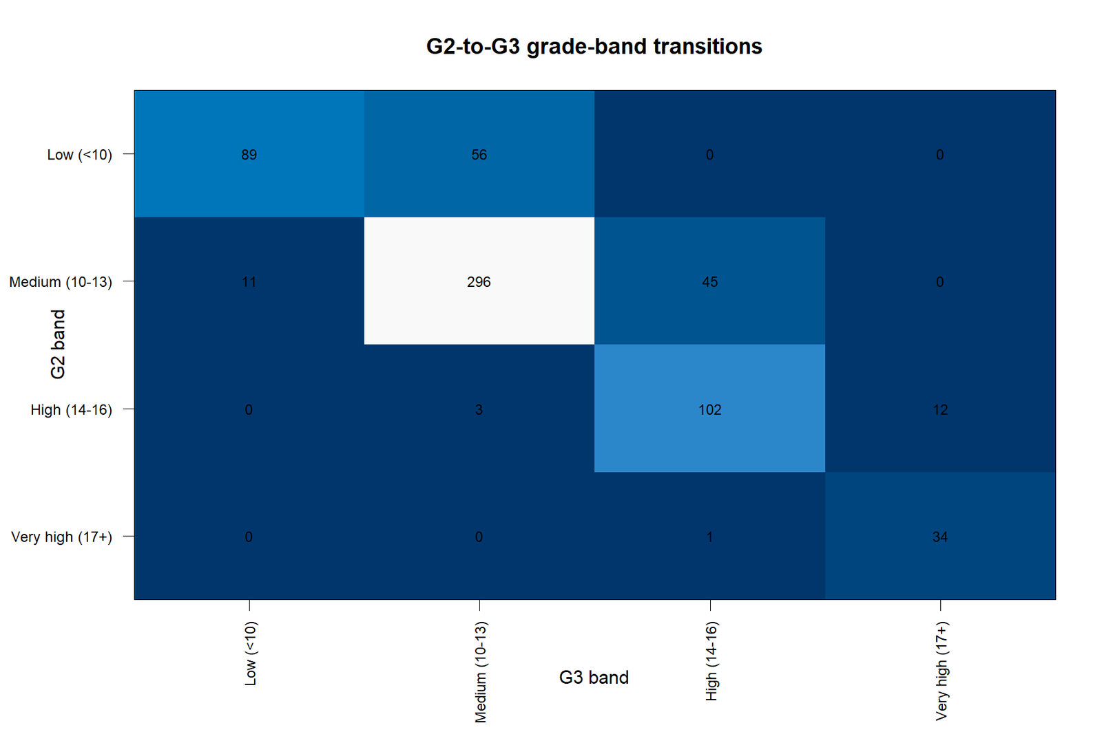
The largest cells are 89, 296, 102 and 34 on the main diagonal, showing substantial stability between G2 and G3 bands.
Off-diagonal direction is still highly uneven
Despite strong diagonal stability, the most visible off-diagonal cells are 1→2, 2→3 and 3→4, not their reverse cells.
Chart pair 2: Asymmetry matrices
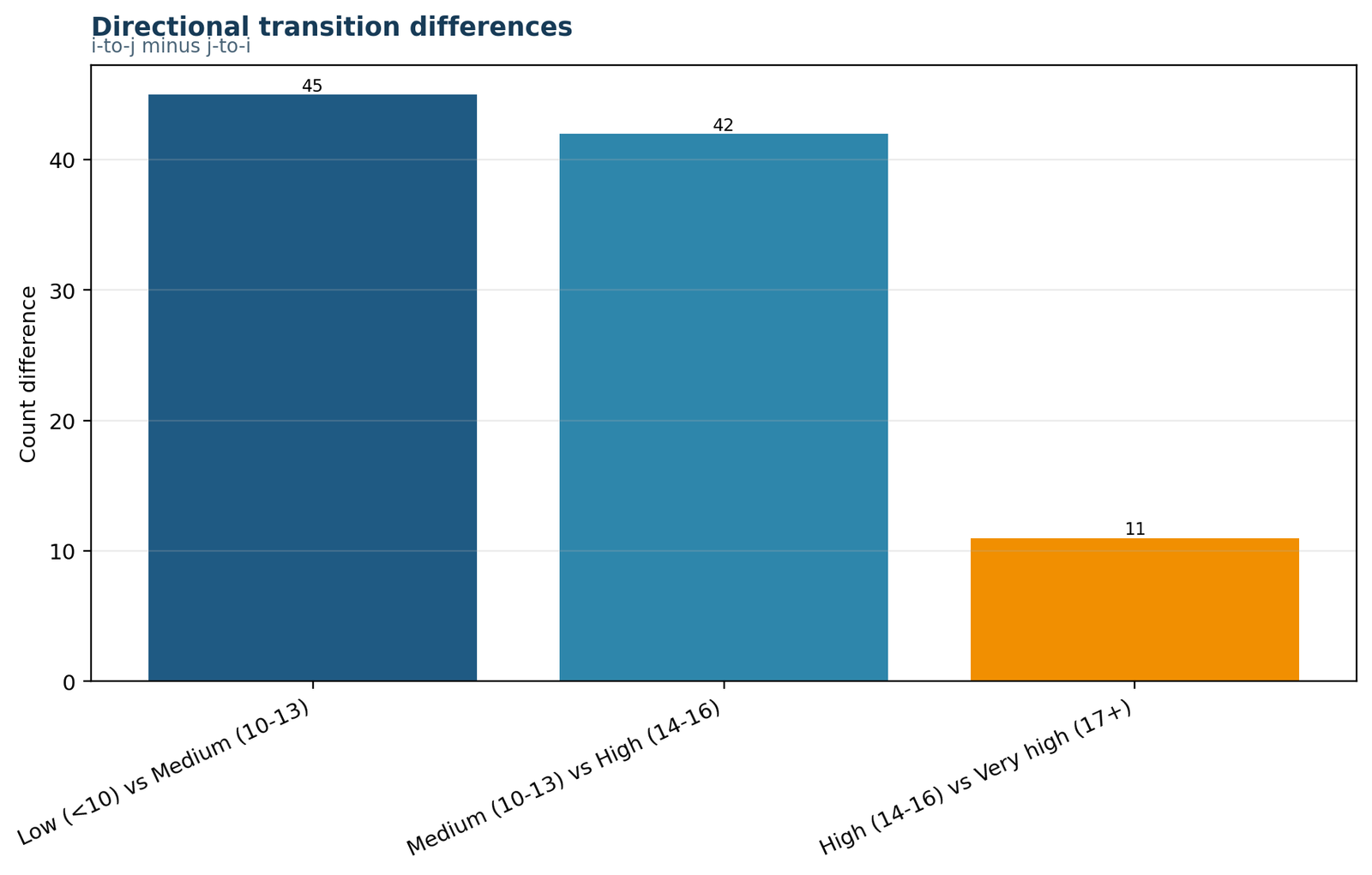
Three adjacent-pair imbalances dominate
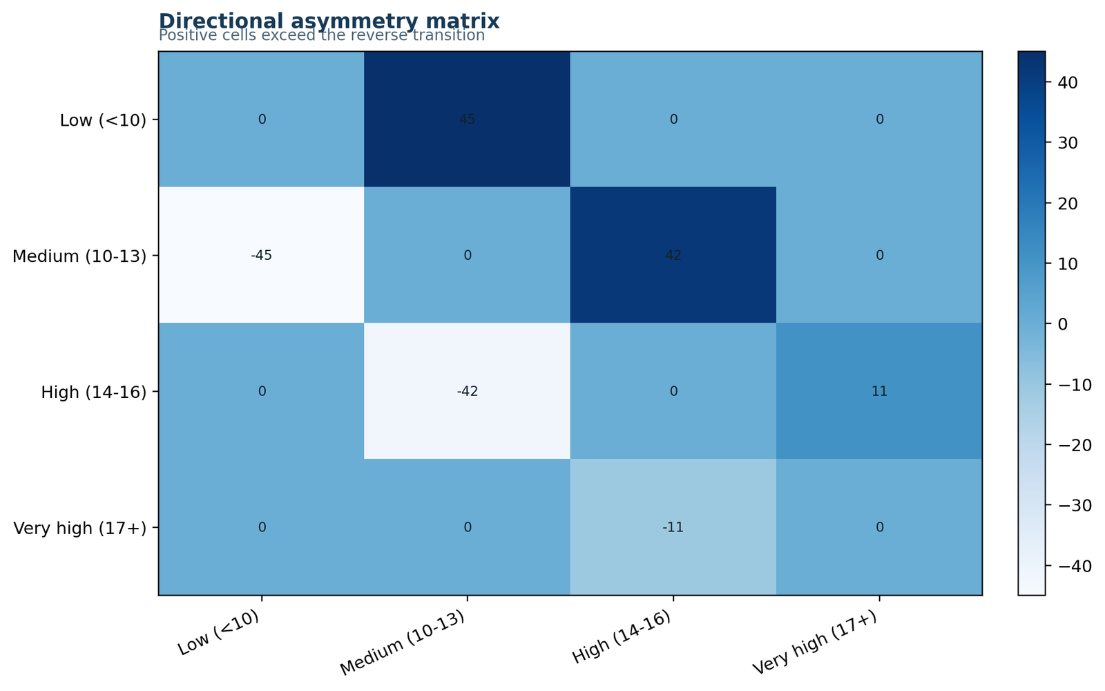
The signed differences are +45 for 1→2, +42 for 2→3 and +11 for 3→4 when upward movement is treated as positive.
The asymmetry has a coherent direction
The result is not produced by random mixed-direction discrepancies. The informative imbalances all point upward.
Chart pair 3: Pair contributions
The 2↔3 pair contributes the most
The contributions are 30.2239, 36.7500 and 9.3077 for the three informative pairs.
The global test is not equally distributed
Nearly half of the asymmetry evidence comes from the strong imbalance between bands 2 and 3.
Chart pair 4: Pair directions
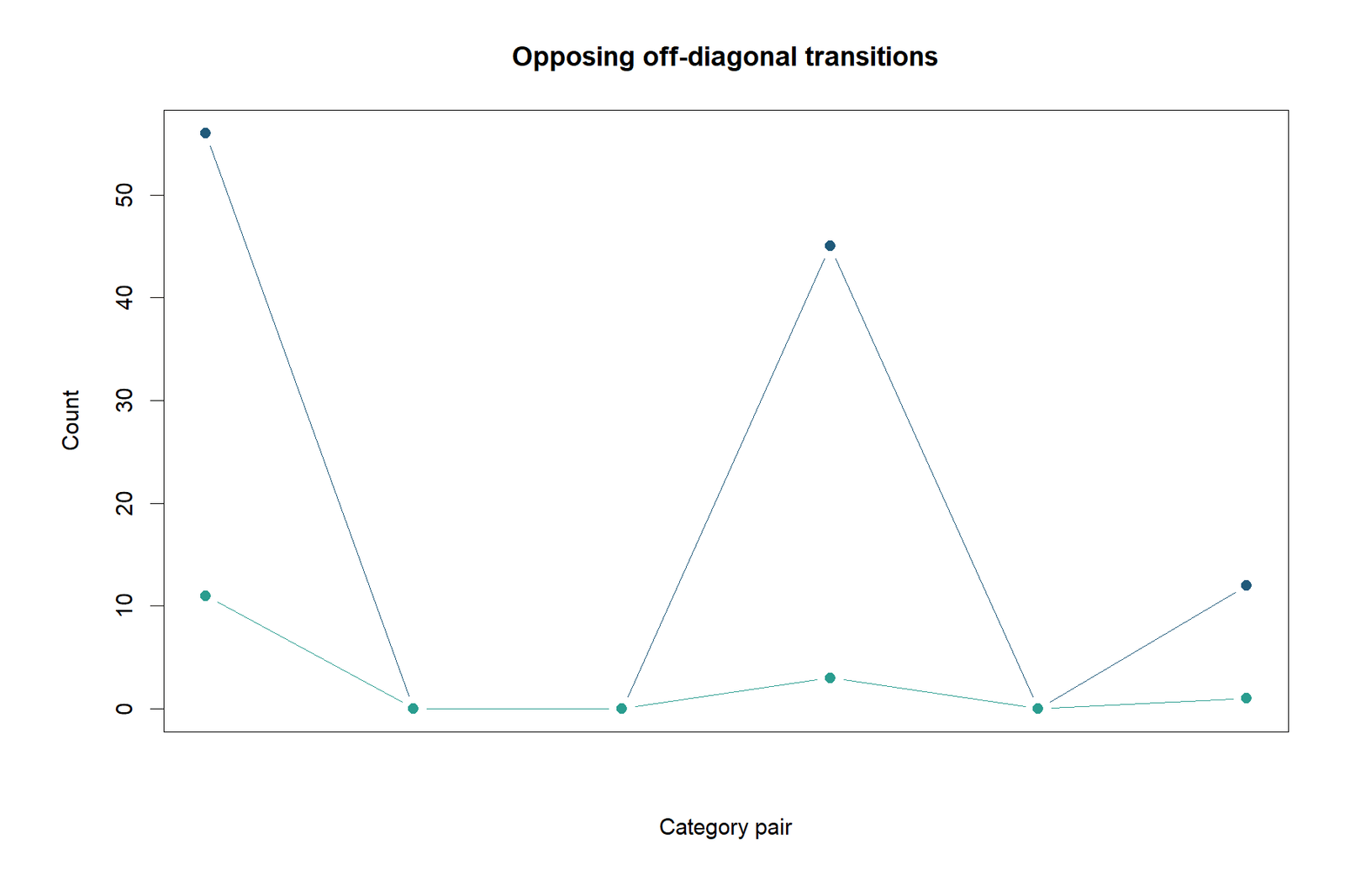
Forward counts exceed reverse counts
The comparisons are 56 versus 11, 45 versus 3 and 12 versus 1.
The result reflects systematic upward movement
The paired table indicates more progression to higher grade bands from G2 to G3 than regression to lower bands.
Chart pair 5: Margins and diagonal agreement
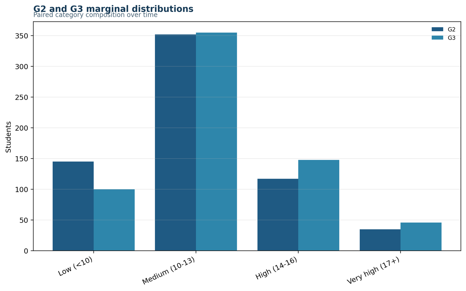
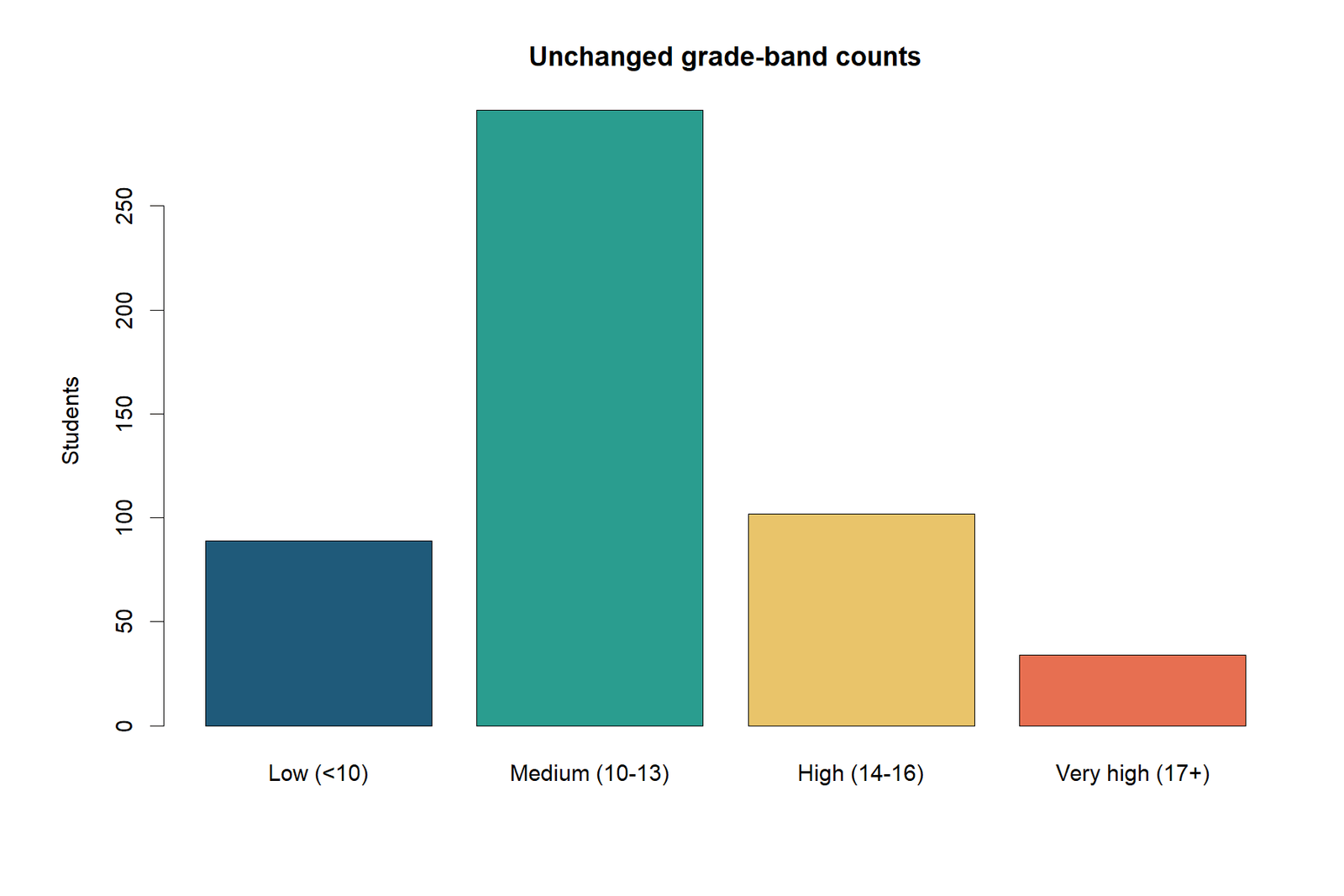
The marginal distribution shifts upward
Band 1 falls from 145 to 100, while bands 3 and 4 increase from 117 to 148 and from 35 to 46.
Stability and change coexist
The diagonal remains dominant, but the off-diagonal flow changes the overall grade-band distribution.
Chart pair 6: Result summary
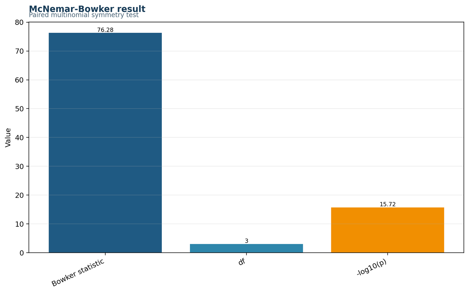
The final decision is decisive
The summary panels combine the statistic, informative degrees of freedom, p-value and rejection decision.
Paired transition symmetry is rejected
The grade-band change pattern cannot be explained as balanced movement in opposite directions.
McNemar Bowker Test in Python, R, SPSS and Excel
McNemar Bowker Test in Python
Python can construct the paired transition matrix, enumerate mirrored pairs, calculate the Bowker statistic and create the transition, asymmetry and contribution charts. For broader categorical workflows, see categorical data analysis in Python.
- Create a square contingency matrix from paired observations.
- Loop over i < j.
- Skip pairs with nij + nji = 0.
- Sum pair contributions.
- Use the informative-pair count for the verified df specification.
McNemar Bowker Test in R
R is well suited to paired transition tables and custom Bowker calculations. It can also reproduce the asymmetry matrix, contribution profile and marginal-change plots. See categorical data analysis in R.
- Build the table with matching factor levels.
- Calculate mirrored-pair terms explicitly.
- Verify the statistic against a suitable package or reference function.
- Count informative pairs consistently.
- Create paired chart diagnostics.
McNemar Bowker Test in SPSS
SPSS can display the paired square table and provide related symmetry output depending on procedure and version. The supplied SPSS PDF is used as a cross-software verification source. See categorical data analysis in SPSS.
- Define the paired G2 and G3 band variables.
- Request the square transition table.
- Verify category order before interpreting direction.
- Compare the symmetry statistic and df with the workbook.
- Export the output PDF.
McNemar Bowker Test in Excel
The worked Excel file contains the original paired variables, transition table, six mirrored-pair comparisons, diagnostic shares and reporting sheet. It is the most transparent way to audit the formula manually.
- Enter the 4 × 4 observed table.
- List every i < j mirrored pair.
- Compute differences, pair totals and contributions.
- Sum contributions to obtain χ²B.
- Use the verified reference p-value when floating-point precision reaches Excel's boundary.
Expandable Code for the McNemar Bowker Test
Python pseudo-code
table = [
    [89, 56, 0, 0],
    [11, 296, 45, 0],
    [0, 3, 102, 12],
    [0, 0, 1, 34]
]
statistic = 0.0
df = 0
for i in range(len(table)):
    for j in range(i + 1, len(table)):
        nij, nji = table[i][j], table[j][i]
        if nij + nji > 0:
            statistic += (nij - nji) ** 2 / (nij + nji)
            df += 1
R pseudo-code
x <- matrix(c(
  89,56,0,0,
  11,296,45,0,
  0,3,102,12,
  0,0,1,34
), nrow=4, byrow=TRUE)
stat <- 0
df <- 0
for (i in 1:3) for (j in (i+1):4) {
  total <- x[i,j] + x[j,i]
  if (total > 0) {
    stat <- stat + (x[i,j] - x[j,i])^2 / total
    df <- df + 1
  }
}
Excel formula idea
Pair contribution = (n_ij - n_ji)^2 / (n_ij + n_ji)
Bowker statistic = SUM(all informative pair contributions)
Informative df = COUNT(pair totals greater than zero)
Assumptions, Limitations and Advanced Interpretation
Assumptions
- The observations are paired.
- Each participant contributes one G2 and one G3 classification.
- The same categories and coding are used at both times.
- Pairs of participants are independent of other pairs.
- The square table is correctly constructed.
- The chi-square approximation is adequate for the informative discordant totals.
Limitations
- The global test does not identify causal reasons for change.
- It does not provide a standard effect-size coefficient.
- Sparse discordant pairs can weaken asymptotic accuracy.
- It tests symmetry, not agreement magnitude.
- It does not adjust for covariates or clustering.
- Category banding can discard information from the original grades.
How zero-total pairs affect the analysis
Pairs 1↔3, 1↔4 and 2↔4 contain no transitions in either direction. Their contribution is mathematically zero. The verified workflow counts only nonzero discordant pairs as informative degrees of freedom, giving df = 3. Analysts should state this convention because some software may display the theoretical maximum df instead.
Asymptotic versus exact inference
The standard Bowker statistic uses a chi-square approximation. When informative discordant totals are very small, an exact or permutation approach may be preferable. In this workbook, the informative pair totals are 67, 48 and 13; the first two are substantial, while the third is smaller but still nonzero.
Ordered-category interpretation
Although Bowker's test is valid as a nominal symmetry test, the ordered grade bands make direction meaningful. The strong excess of upward transitions gives a clearer substantive story than a nominal-label application would provide.
APA Reporting for the McNemar Bowker Test
Filled APA result
Significant
A McNemar Bowker Test was conducted to examine symmetry in the paired four-category G2-to-G3 grade-band transition table.
The transition matrix was significantly asymmetric, χ²B(3, N = 649) = 76.28, p < .001.
Upward transitions were substantially more frequent than their reverse transitions, particularly for bands 1↔2 and 2↔3.
Report the row-to-column time order and explain why df = 3 when zero-total pairs are excluded.
Reusable APA template
Template
A McNemar Bowker Test was used to evaluate symmetry in the paired [k × k classification table].
The symmetry result was [significant/not significant], χ²B([df], N = [N]) = [statistic], p = [p-value].
The largest directional imbalance occurred between [category pair], with [n_ij] transitions in one direction and [n_ji] in the reverse direction.
Use p < .001 rather than printing a long string of zeros in APA prose.
Direction-focused report
Ordered categories
Of the 128 students who changed grade band, 113 moved upward and 15 moved downward.
The significant McNemar Bowker Test therefore reflected systematic upward rather than balanced bidirectional movement.
Common McNemar Bowker Test Mistakes and How to Correct Them
Common mistakes
- Using independent groups instead of paired classifications.
- Running an ordinary chi-square independence test on the paired matrix.
- Interpreting diagonal agreement as evidence of symmetry.
- Ignoring the direction of mirrored-pair differences.
- Reporting df = 6 without checking zero-total pairs.
- Calling the result an agreement coefficient.
How to correct them
- Confirm that each row and column value belongs to the same participant.
- Use the mirrored-pair Bowker formula.
- Separate agreement description from symmetry inference.
- Report the informative pair counts and directions.
- State the software or workbook df convention.
- Use kappa separately when agreement magnitude is the goal.
McNemar Bowker Test Reports and Worked Excel Download
R PDF reportR calculation and chart workflow for the same paired table.
SPSS PDF outputSPSS cross-software verification output.
Worked Excel analysisComplete input, observed table, calculations, diagnostics and reporting sheets.
Frequently Asked Questions About the McNemar Bowker Test
What is the McNemar Bowker Test?
It is a paired multi-category test that evaluates whether every off-diagonal transition count equals its mirrored reverse-transition count in a square table.
How is it different from the ordinary McNemar test?
The ordinary McNemar test handles two categories. The McNemar Bowker Test extends the same symmetry principle to three or more categories.
What does a significant McNemar Bowker Test mean?
It means at least one category transition occurs more often in one direction than in the reverse direction. It does not by itself mean agreement is low.
Why is df equal to 3 in this four-category example?
Although six mirrored pairs are theoretically possible, only three have nonzero discordant totals. The verified workflow counts those three informative pairs.
Which pairs drive the result?
The 2↔3 pair contributes 48.18% of the statistic, the 1↔2 pair contributes 39.62%, and the 3↔4 pair contributes 12.20%.
What is the final conclusion?
The G2-to-G3 grade-band transition matrix is strongly asymmetric, with 113 upward transitions and 15 downward transitions.
McNemar Bowker Test Conclusion
McNemar Bowker Test is the appropriate extension of McNemar's paired binary method when the same participants are classified into three or more matching categories at two occasions. It tests whether each transition direction is balanced by its reverse direction and therefore reveals systematic change that a simple agreement percentage can miss.
In this worked analysis of 649 students, 521 remained in the same grade band, but the 128 changes were highly directional: 113 upward and only 15 downward. The verified result, χ²B(3, N = 649) = 76.28, p < .001, rejects transition symmetry decisively. The main evidence came from the 1↔2 and 2↔3 pairs, with an additional contribution from 3↔4.
For the next step, compare the symmetry result with Cohen's Kappa for agreement magnitude, Bowker's Test of Symmetry for related worked interpretation and Categorical Data Analysis in Python for a broader software workflow.

