
Breslow-Day Test: Formula, Interpretation, Python, R, SPSS and Excel Guide
The Breslow-Day Test evaluates whether stratum-specific odds ratios can reasonably be treated as homogeneous. This complete public guide explains the null hypothesis, common-odds model, Tarone adjustment, calculator steps, assumptions, worked four-stratum example, Python and R charts, SPSS and Excel workflows, APA reporting, common mistakes, and downloadable analysis files.
Four study-time strata
Breslow-Day Test χ²(3) = 3.442
p = .328
Common OR = 0.800
Breslow-Day Test: Model Overview
Definition and Purpose
The Breslow-Day Test is a chi-square homogeneity test for a collection of stratified 2 × 2 contingency tables. It asks whether the odds ratio linking a binary exposure and binary outcome is constant across the levels of a stratifying variable.
In this example, the exposure is sex, the outcome is G3 ≥ 10, and the strata are four studytime levels. The question is not whether sex and passing are associated overall; it is whether the sex–pass odds ratio changes materially across study-time strata.
Research Question and Null Model
Research question: Are the male-versus-female odds ratios for passing homogeneous across study-time levels 1 through 4?
The common odds ratio estimate is 0.799912. The Breslow-Day Test statistic measures how far each observed stratum table departs from the table expected under that common-odds model.
When the Test Is Needed
Use the Breslow-Day Test before emphasizing a single Mantel–Haenszel common odds ratio. A nonsignificant homogeneity test supports a common-effect summary, while a significant test warns that one pooled odds ratio can conceal effect modification.
What the Test Does Not Test
The Breslow-Day Test does not test whether the common odds ratio equals 1. It also does not prove that all odds ratios are identical. The common-effect association requires a separate Cochran–Mantel–Haenszel or equivalent test.
Worked Conclusion
The verified result is χ²(3) = 3.441983, p = 0.328365. The null hypothesis is not rejected. The four observed odds ratios are statistically compatible with a common effect, although the smallest stratum is imprecise and requires cautious interpretation.
Quick Answer: Breslow-Day Test Result
Homogeneity Decision
- Null: all four odds ratios are homogeneous.
- Alpha: .05.
- Decision: fail to reject H0.
- Meaning: observed differences between stratum odds ratios are compatible with sampling variation.
Common-Effect Context
- Mantel–Haenszel common OR: 0.799912.
- 95% CI: [0.510177, 1.254189].
- Common OR = 1 test: χ² = 0.9333, p = 0.3340.
- Interpretation: no significant overall common association was detected.
Largest contribution: stratum 4 = 2.584
Total N = 649
Minimum stratum N = 35
Table of Contents
What Is the Breslow-Day Test?
A Test of Effect Homogeneity
The Breslow-Day Test evaluates a collection of independent 2 × 2 tables created by stratifying on a third variable. Each table estimates an exposure–outcome odds ratio. The test compares the observed cell counts with counts expected if all strata shared one common odds ratio.
The procedure is often used with the Mantel–Haenszel method. The homogeneity test determines whether a pooled odds ratio is defensible; the Mantel–Haenszel analysis estimates and tests that pooled effect.
A Test of Interaction on the Odds-Ratio Scale
A significant Breslow-Day Test suggests that the exposure effect varies across strata. In modern modelling language, this is evidence of effect modification or an interaction on the log-odds scale. A nonsignificant result means that the available data do not establish such heterogeneity.
The result depends on stratum size and precision. Large numerical differences can remain nonsignificant when small strata produce wide uncertainty.
Exposure
Sex is coded as male versus female. The odds ratio is calculated as male pass odds divided by female pass odds.
Outcome
G3 is converted to a binary final-pass outcome: pass when G3 ≥ 10 and fail when G3 < 10.
Stratifier
Study time has four ordered levels. A separate 2 × 2 sex-by-pass table is formed inside each level.
Why Four Separate Odds Ratios Are Not Enough
Simply listing 0.721, 0.927, 1.826 and a zero-cell estimate does not establish heterogeneity. The estimates have very different precision because the stratum sizes are 212, 305, 97 and 35. The fourth stratum has a zero female-fail cell, and the third and fourth confidence intervals are very wide. The Breslow-Day Test weights the observed departures through their model-based variances rather than comparing point estimates visually.
Interpretation of a Nonsignificant Result
A nonsignificant Breslow-Day Test supports using a common-odds interpretation, but it does not prove exact equality. The phrase “no evidence of heterogeneity” is more accurate than “the odds ratios are the same.” Power can be limited when there are few strata, small cells, zero cells, or modest interaction effects.
Research Question, Hypotheses and Stratified Design
Research Question
Does the male-versus-female odds ratio for G3 ≥ 10 remain constant across four study-time levels?
Null Hypothesis
H0: θ1 = θ2 = θ3 = θ4. A common odds-ratio model adequately describes all strata.
Alternative Hypothesis
H1: at least one θh differs. The exposure–outcome association is modified by study time.
Design Structure
Male/female exposure and pass/fail outcome.
Build four independent 2 × 2 tables.
Compare observed and common-model expected counts.
Sampling Units and Independence
Each student contributes to one study-time stratum and one sex-by-pass cell. Students should be independent within and between strata. The test does not accommodate repeated observations, matched pairs, or cluster dependence without additional modelling.
Direction of the Odds Ratio
The tables define the odds ratio as:
An odds ratio below 1 indicates lower male pass odds relative to female pass odds within that stratum. Reversing the exposure or outcome changes the numerical direction but not the homogeneity conclusion when done consistently.
Why the Strata Must Be Prespecified
Study-time categories should be defined before examining the odds ratios. Searching many possible stratifications and reporting the one with the most striking heterogeneity inflates false-positive risk. See Null and Alternative Hypothesis and Type I and Type II Error for the general logic of prespecified testing.
When to Use the Breslow-Day Test
Use the Breslow-Day Test When
- There are two binary variables in every stratum.
- The strata are mutually exclusive.
- Observations are independent within and across strata.
- The effect measure of interest is an odds ratio.
- A common Mantel–Haenszel odds ratio is being considered.
- Effect modification by a categorical stratifier is scientifically relevant.
- There are enough observations to support the chi-square approximation.
- Table orientation is identical across strata.
Choose Another Method When
- The outcome or exposure has more than two categories.
- Observations are paired, repeated or clustered.
- The effect measure of interest is a risk difference or risk ratio.
- Continuous or multi-level effect modifiers should be modelled directly.
- There are many covariates requiring simultaneous adjustment.
- Several strata are extremely sparse or structurally zero.
- The study estimates subject-specific rather than marginal effects.
- The main task is prediction rather than homogeneity testing.
Small Numbers of Strata
The test can be used with a small number of strata, but power to detect moderate heterogeneity may be limited. Degrees of freedom equal the number of strata minus one.
Sparse Strata
Zero or near-zero cells can produce unstable stratum odds ratios. A continuity correction may help visualization, but it does not erase the underlying information limitation.
Regression Alternative
A logistic regression with an exposure-by-stratum interaction can test and estimate effect modification while accommodating additional covariates.
Breslow-Day Test Formula and Worked Calculation
Observed Cell a
For each stratum, ah is the exposed-positive cell. In the current orientation, it is the male-pass count. The observed values are 91, 92, 21 and 12.
Expected Cell E(a)
Eh is the male-pass count expected under the common odds ratio θ = 0.799912, while preserving the stratum margins. The expected values are 91.9364, 90.7722, 20.1451 and 13.0973.
Expected Cell Under the Common Odds Ratio
Let m1h be the exposed row total, n1h the positive-outcome column total, Nh the stratum total, and θ the common odds ratio. The expected cell x solves the quadratic:
The feasible root within the table margins is used. The conditional variance of that expected cell supplies the denominator of each contribution.
Worked Contributions
| Stratum | Observed a | Expected a | Variance | Observed − expected | Contribution |
|---|---|---|---|---|---|
| 1 | 91 | 91.936428 | 9.078517 | −0.936428 | 0.096590 |
| 2 | 92 | 90.772235 | 8.418934 | +1.227765 | 0.179050 |
| 3 | 21 | 20.145089 | 1.254037 | +0.854911 | 0.582816 |
| 4 | 12 | 13.097290 | 0.466047 | −1.097290 | 2.583527 |
Decision Rule
Under the homogeneity null and suitable large-sample conditions, QBD is compared with a chi-square distribution having H − 1 degrees of freedom. Here, χ²(3) = 3.441983 and p = .328365. Because p exceeds .05, the data do not establish odds-ratio heterogeneity.
Variables and Data Dictionary
| Variable | Role | Coding | Valid N | Interpretive function |
|---|---|---|---|---|
| sex | Binary exposure | Female versus male | 649 | Defines exposure rows in every 2 × 2 stratum table. |
| G3 | Original quantitative outcome | Final grade | 649 | Source of the binary pass/fail outcome. |
| G3 ≥ 10 | Binary outcome | 1 = pass; 0 = fail | 649 | Defines outcome columns. |
| studytime | Stratifying variable | Levels 1, 2, 3 and 4 | 649 | Creates four separate sex-by-pass tables. |
Level 1
<2 study hours per week. N = 212.
Level 2
2–5 study hours per week. N = 305.
Level 3
5–10 study hours per week. N = 97.
Level 4
>10 study hours per week. N = 35.
Overall Descriptive Context
Male Students
216 of 266 male students passed, a proportion of 0.812030 (81.2%). There were 50 male failures.
Female Students
333 of 383 female students passed, a proportion of 0.869452 (86.9%). There were 50 female failures.
Observed Stratified 2 × 2 Tables
Each study-time level has its own male/female by pass/fail table. The Breslow-Day Test uses all four tables simultaneously while preserving each stratum's margins.
| Study-time stratum | Male pass | Male fail | Female pass | Female fail | Stratum N |
|---|---|---|---|---|---|
| 1 (<2 hours/week) | 91 | 32 | 71 | 18 | 212 |
| 2 (2–5 hours/week) | 92 | 15 | 172 | 26 | 305 |
| 3 (5–10 hours/week) | 21 | 1 | 69 | 6 | 97 |
| 4 (>10 hours/week) | 12 | 2 | 21 | 0 | 35 |
| Total | 216 | 50 | 333 | 50 | 649 |
Stratum-Specific Pass Proportions
- Stratum 1: male 74.0%, female 79.8%.
- Stratum 2: male 86.0%, female 86.9%.
- Stratum 3: male 95.5%, female 92.0%.
- Stratum 4: male 85.7%, female 100.0%.
Information Pattern
Strata 1 and 2 supply most observations. Stratum 3 is smaller and stratum 4 is very small. The female-fail zero in stratum 4 makes its individual odds ratio unstable, but the Breslow-Day Test contribution remains finite because the expected-cell method works with the complete stratum margins and common odds ratio.
Breslow-Day Test Results and Interpretation
Breslow-Day Test
3.441983
χ² with 3 degrees of freedom.
P-Value
0.328365
Fail to reject homogeneity at .05.
Tarone Adjustment
3.441859
Adjusted p = 0.328382.
Common OR
0.799912
95% CI [0.510, 1.254].
Stratum-Specific Effect Estimates
| Study-time stratum | Raw OR | Display OR | 95% lower | 95% upper | Log OR | Contribution |
|---|---|---|---|---|---|---|
| 1 | 0.720951 | 0.720951 | 0.374272 | 1.388750 | −0.327185 | 0.096590 |
| 2 | 0.927132 | 0.927132 | 0.467793 | 1.837510 | −0.075660 | 0.179050 |
| 3 | 1.826087 | 1.826087 | 0.207943 | 16.036100 | 0.602175 | 0.582816 |
| 4 | 0.000000 | 0.116279* | 0.005158 | 2.621270 | −2.151760* | 2.583527 |
*Stratum 4's plot estimate and interval use a continuity correction because the female-fail cell is zero. The raw cross-product odds ratio is 0.
Most Stable Estimate
Stratum 2 has the largest N and an odds ratio near 1. Its contribution is only 0.179, indicating close agreement with the common-odds model.
Largest Point Estimate
Stratum 3 has OR = 1.826, but the interval is extremely wide. The small number of failures limits precision, and its contribution remains only 0.583.
Largest Heterogeneity Contribution
Stratum 4 contributes 2.584, or 75.1% of QBD. Its small N and zero cell produce the largest model departure but not enough total evidence to reject homogeneity.
Interpretation of p = .328
The observed variation in odds ratios is not larger than expected under a common-odds model. This result supports summarizing the association with a common odds ratio, provided that the common effect is scientifically meaningful and the small fourth stratum is discussed. The result does not show that the stratum odds ratios are numerically identical, and it does not guarantee high power to detect modest effect modification.
Common Odds Ratio and Cochran–Mantel–Haenszel Context
Mantel–Haenszel Common Odds Ratio
The estimated common odds ratio is 0.799912. On the chosen scale, male pass odds are estimated at approximately 80% of female pass odds after stratifying by study time.
The 95% confidence interval is [0.510177, 1.254189]. Because it includes 1, the common association is not statistically significant.
Separate Test of the Common Effect
The test of a common odds ratio equal to 1 gives χ² = 0.933256, p = 0.334018. This is conceptually separate from the Breslow-Day Test.
Homogeneity question: do the odds ratios vary across strata?
Association question: is the common odds ratio different from 1?
Possible Outcome A
Homogeneous and significant: one common non-null effect is a useful summary.
Possible Outcome B
Homogeneous and nonsignificant: one common estimate may be used, but the data do not establish an association.
Possible Outcome C
Heterogeneous: emphasize stratum-specific effects or an interaction model rather than one pooled odds ratio.
The worked example fits outcome B. The Breslow-Day Test is nonsignificant, and the common odds ratio test is also nonsignificant. The most accurate conclusion is that there is no detected effect modification by study time and no detected common sex effect on pass odds after stratification.
Tarone-Adjusted Breslow-Day Test
Why Tarone Adjustment Exists
The ordinary Breslow-Day Test statistic can deviate slightly from its intended chi-square behaviour because the common odds ratio is estimated from the same tables. Tarone's adjustment removes a component related to the total observed-minus-expected deviation and improves the asymptotic calibration.
Worked Tarone Result
The unadjusted statistic is 3.441983431. The Tarone-adjusted statistic is 3.441858707. Their difference is only 0.000124725.
The adjusted p-value is 0.328381509, almost identical to the unadjusted p-value of 0.328364995.
Because the adjustment is negligible in this dataset, both versions lead to the same conclusion. Reporting both can be useful for reproducibility, especially when software provides a Tarone option. The article should not describe Tarone's adjustment as a different substantive hypothesis; it is a calibration adjustment for the same homogeneity question.
Breslow-Day Test Calculator: Step-by-Step Workflow
Calculator Inputs
Four consistently oriented 2 × 2 tables, one for each study-time stratum, plus an alpha level and a zero-cell policy for descriptive odds-ratio displays.
Required Intermediate Values
Common odds ratio, expected exposed-positive cell in each stratum, conditional variance, observed-minus-expected deviation and contribution.
Required Outputs
Breslow-Day Test statistic, df, p-value, Tarone-adjusted result, common odds ratio, interval and a table of stratum diagnostics.
Calculator Steps
1. Enter the Four Tables
Use the same exposure and outcome orientation in every stratum. Check that all counts are nonnegative integers and that the stratum totals sum to 649.
2. Estimate the Common OR
Compute the Mantel–Haenszel common odds ratio. The worked result is 0.799911650.
3. Solve Expected a
For each stratum, solve the common-odds quadratic and retain the root permitted by the fixed row and column margins.
4. Calculate Variance
Use the model-based conditional variance of a under the common-odds null.
5. Sum Contributions
Add (a − E[a])²/Var(a). The four contributions sum to 3.441983431.
6. Obtain the P-Value
Use the right tail of χ² with H − 1 = 3 degrees of freedom. The result is p = 0.328364995.
Calculator Validation Targets
BD = 3.441983431
df = 3
p = 0.328364995
Tarone = 3.441858707
Tarone p = 0.328381509
Six Python Breslow-Day Test Chart Stories
The Python charts are presented in a separate software section. They move from stratum-specific estimates and counts to heterogeneity profiles, log effects and the final test summary. Each pair is arranged horizontally to keep the desktop article compact.
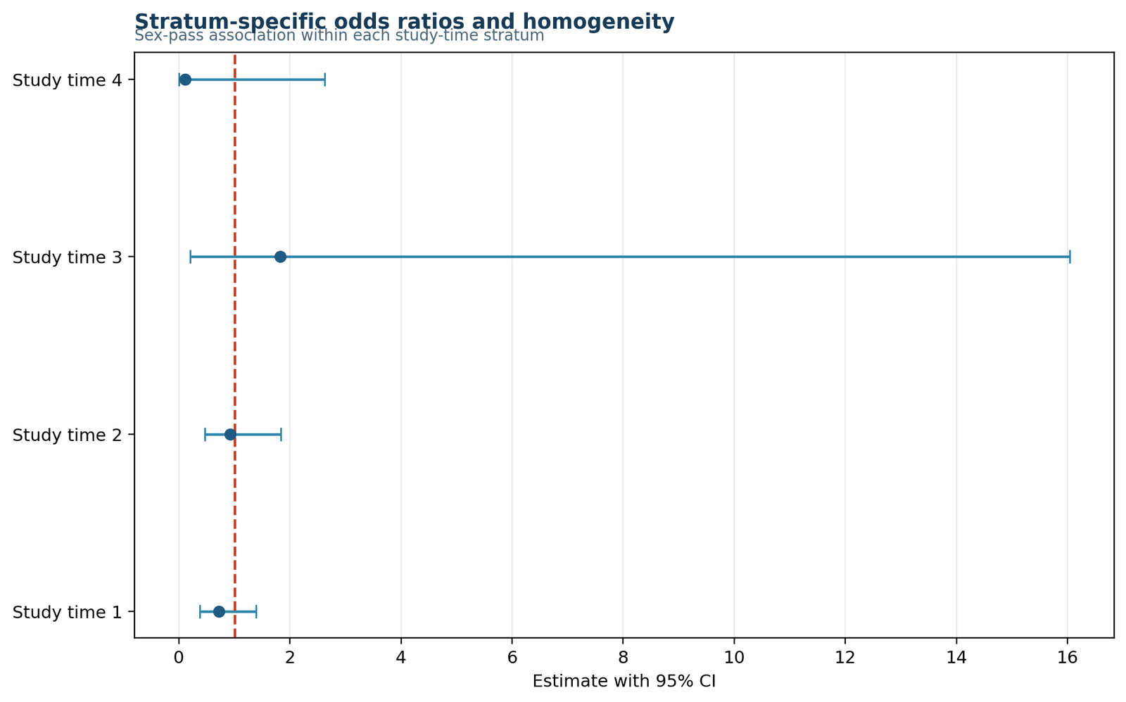
Stratum-Specific Odds Ratios and Homogeneity
Pattern: The first two estimates lie below 1, the third lies above 1, and the corrected fourth estimate lies far below 1. Every interval includes 1.
Interpretation: The point estimates vary, but the third and fourth strata are highly imprecise. Visual spread alone is not sufficient evidence of heterogeneity.
Next step: Read the forest plot with the Breslow-Day Test p-value and stratum sizes.
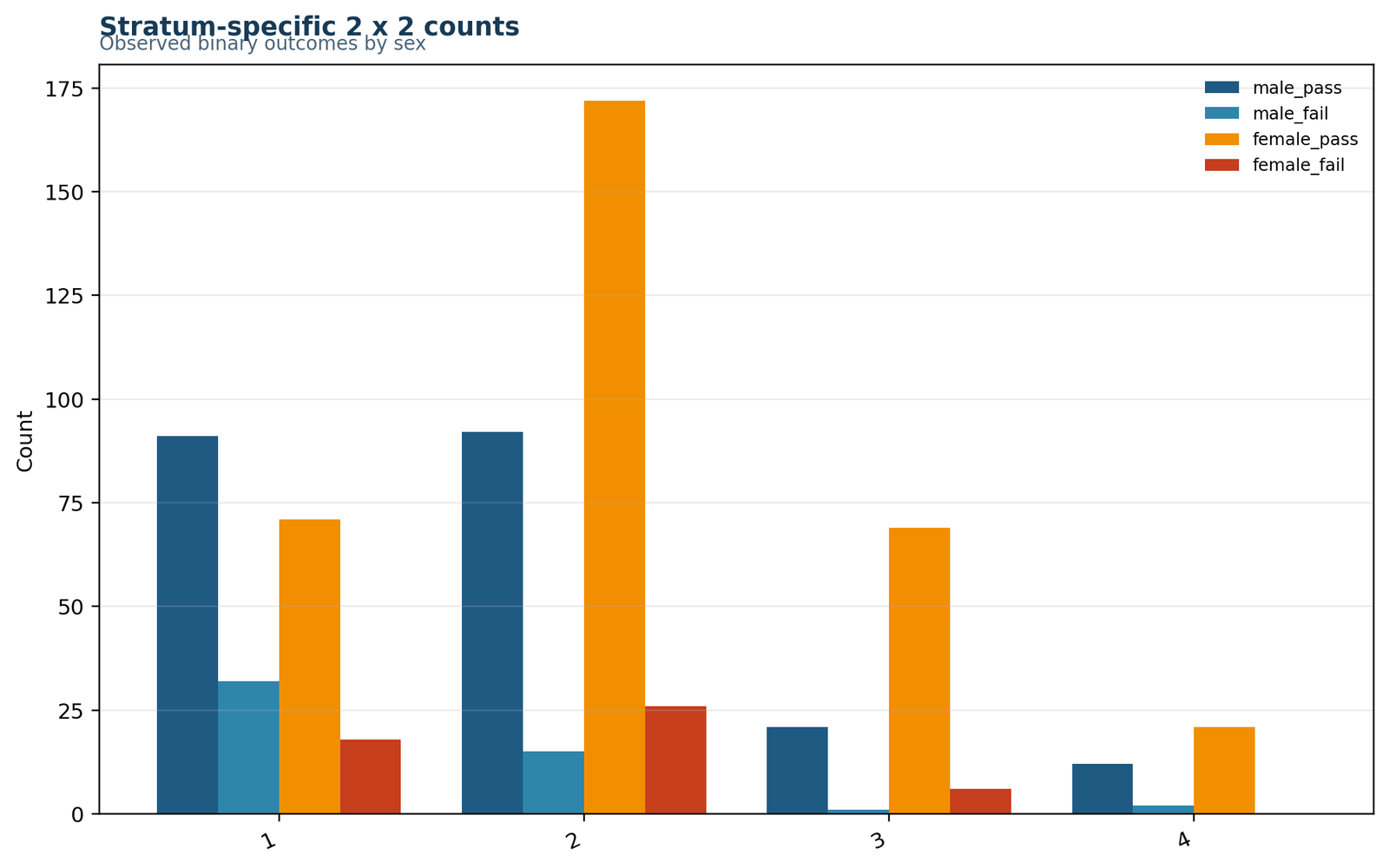
Stratum-Specific 2 × 2 Counts
Pattern: Study-time level 2 is the largest stratum. Levels 3 and 4 contain few failures, and level 4 has no female failures.
Interpretation: The uneven information explains the very different confidence-interval widths. Stratum 4 can show a large point deviation while remaining statistically weak.
Next step: Inspect sparse cells before interpreting individual odds ratios.
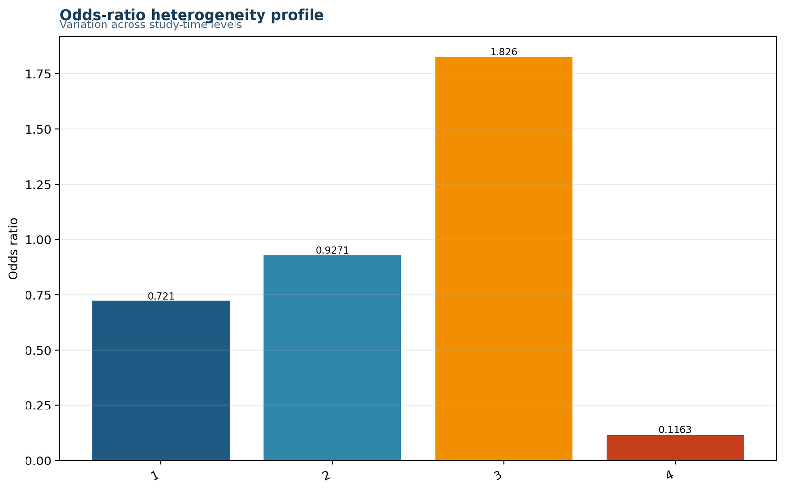
Odds-Ratio Heterogeneity Profile
Pattern: The third stratum has the largest raw nonzero odds ratio, while the corrected fourth estimate is the smallest.
Interpretation: The profile highlights numerical variability but omits precision. The Breslow-Day Test incorporates expected-cell variance and therefore gives a more defensible homogeneity assessment.
Next step: Compare the bar pattern with confidence intervals and contribution values.
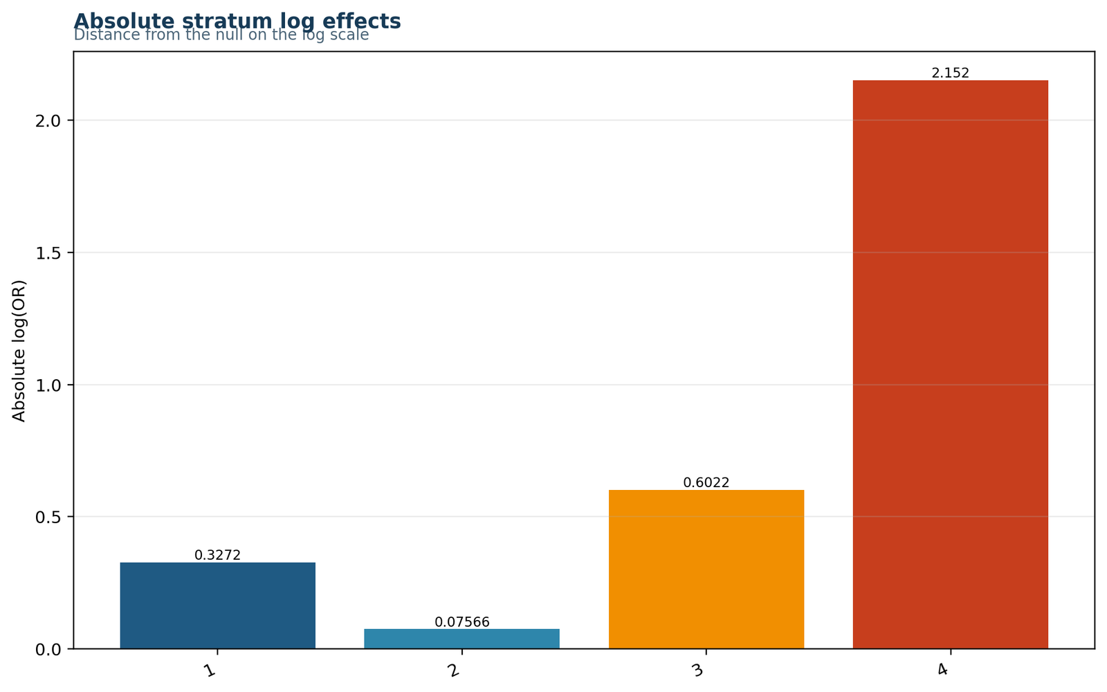
Absolute Log-Effect Magnitudes
Pattern: Stratum 4 is farthest from zero, followed by stratum 3. Stratum 2 is very close to the null.
Interpretation: Absolute log effects measure point-estimate distance, not evidence. A large distance in a small sparse stratum can still have a wide interval and modest inferential weight.
Next step: Do not rank statistical importance from absolute log effects alone.
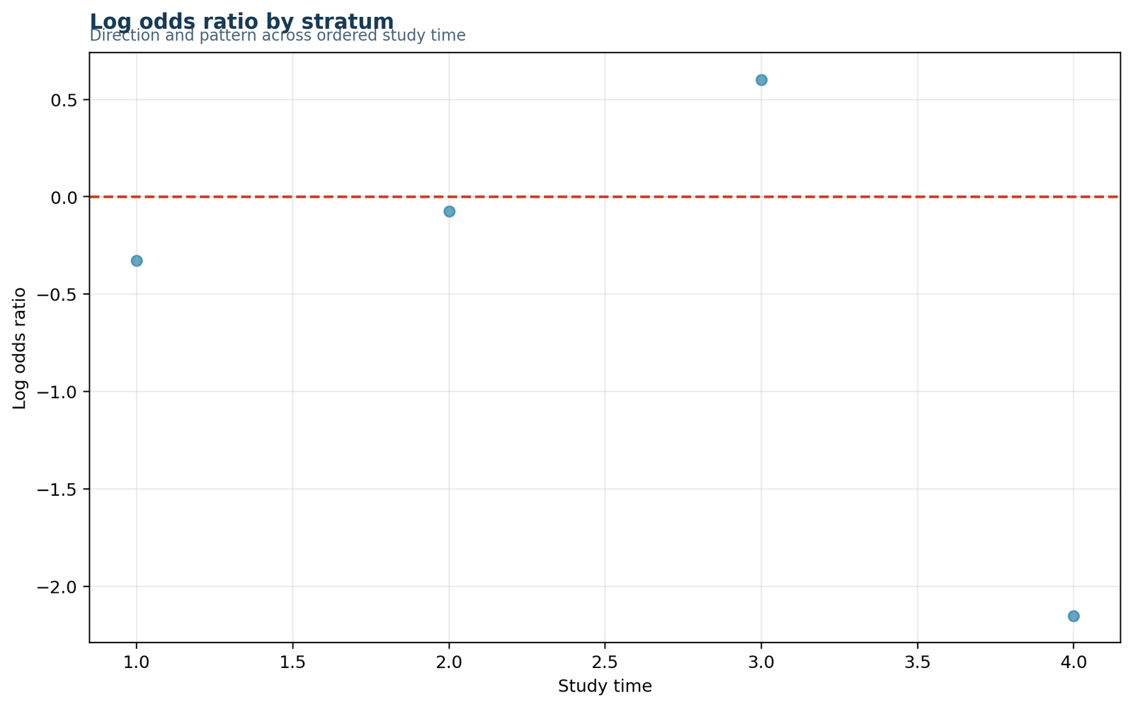
Signed Log Odds Ratios
Pattern: Strata 1, 2 and 4 are negative, while stratum 3 is positive. The sign reversal suggests possible interaction but must be judged with uncertainty.
Interpretation: A sign change can be scientifically interesting, yet the wide intervals in the smaller strata prevent the global homogeneity test from rejecting.
Next step: Consider a logistic interaction model when directional differences are central.
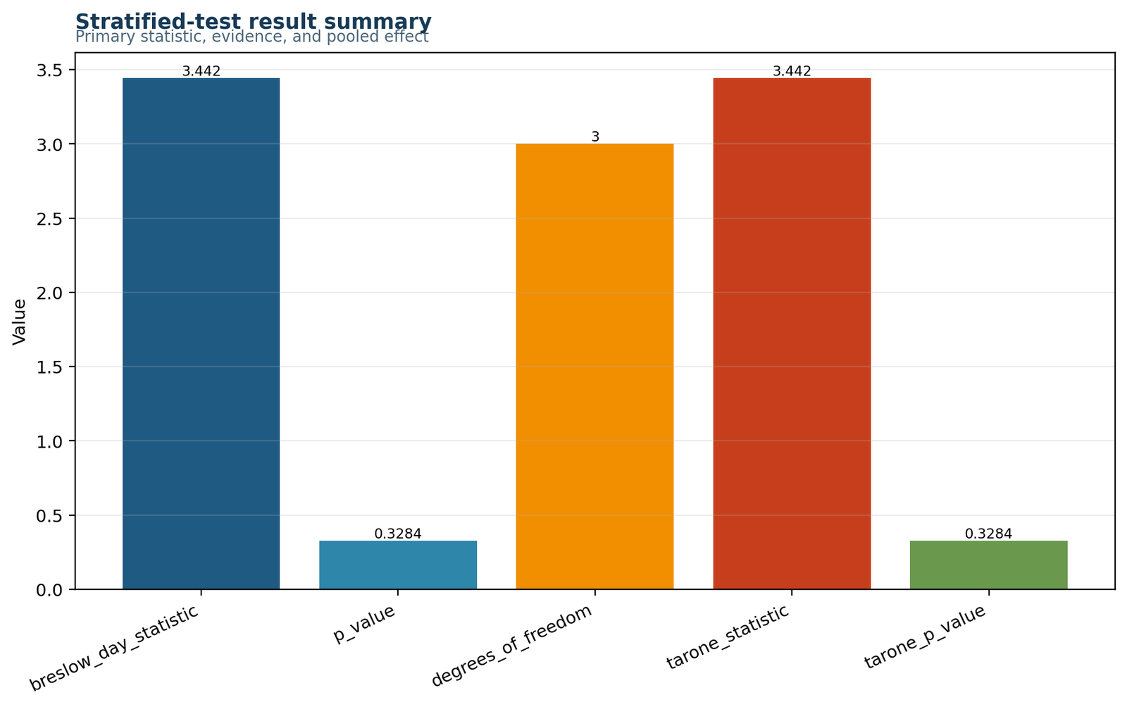
Stratified-Test Result Summary
Pattern: The unadjusted and adjusted statistics are visually indistinguishable, and both p-values are about .328.
Interpretation: Tarone adjustment has a negligible effect. Both analyses support the same nonsignificant homogeneity conclusion.
Next step: Report one primary homogeneity result and optionally add the Tarone sensitivity result.
Six R Breslow-Day Test Charts with Paired Explanations
The R charts appear separately, including the two image URLs that match the Python forest and result-summary figures. Every R figure is displayed in its own R section because software-specific chart sections must remain complete even when published media URLs overlap.
R Stratum Odds Ratios
Pattern: The R forest plot reproduces the Python estimates and demonstrates the wide uncertainty in study-time levels 3 and 4.
Interpretation: Cross-software agreement in estimates is useful, but the formal homogeneity decision comes from the Breslow-Day Test statistic.
Next step: State the continuity correction used for the zero-cell stratum.
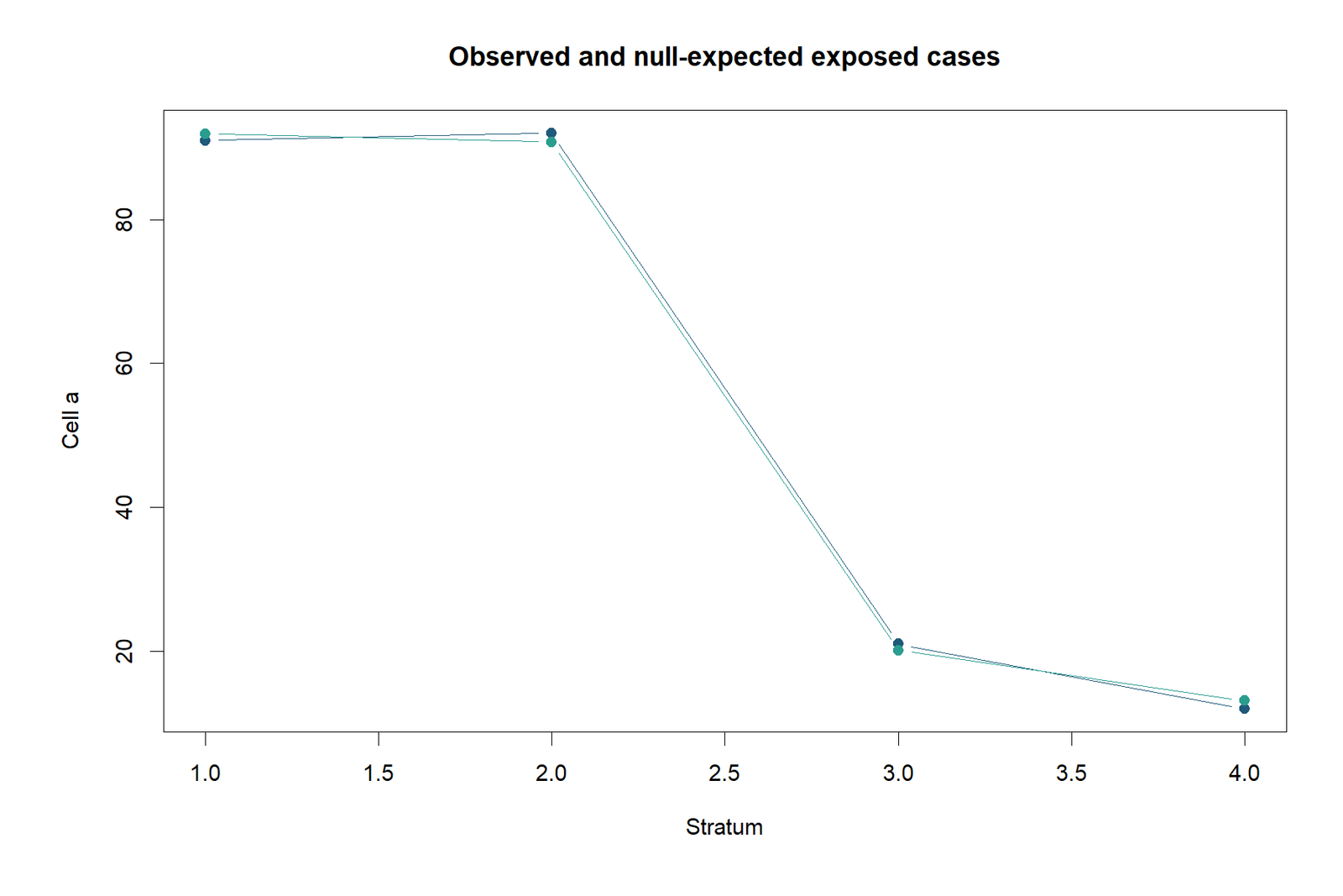
Observed and Null-Expected Cell a
Pattern: Observed and expected values are close in every stratum. The largest absolute gap is about 1.23 in stratum 2.
Interpretation: The Breslow-Day Test statistic is built from these deviations after scaling by conditional variance. Small count gaps can matter differently depending on precision.
Next step: Read each deviation together with its variance and contribution.
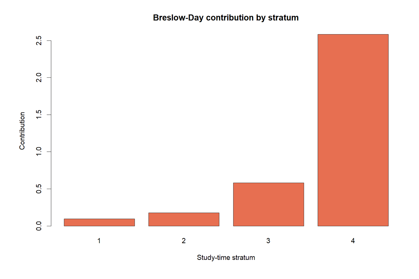
Heterogeneity Contributions
Pattern: Stratum 4 dominates the statistic, while strata 1 and 2 contribute very little.
Interpretation: The smallest stratum creates the largest standardized departure. Even so, the total chi-square remains nonsignificant with three degrees of freedom.
Next step: Discuss influential strata without deleting them solely because they are inconvenient.
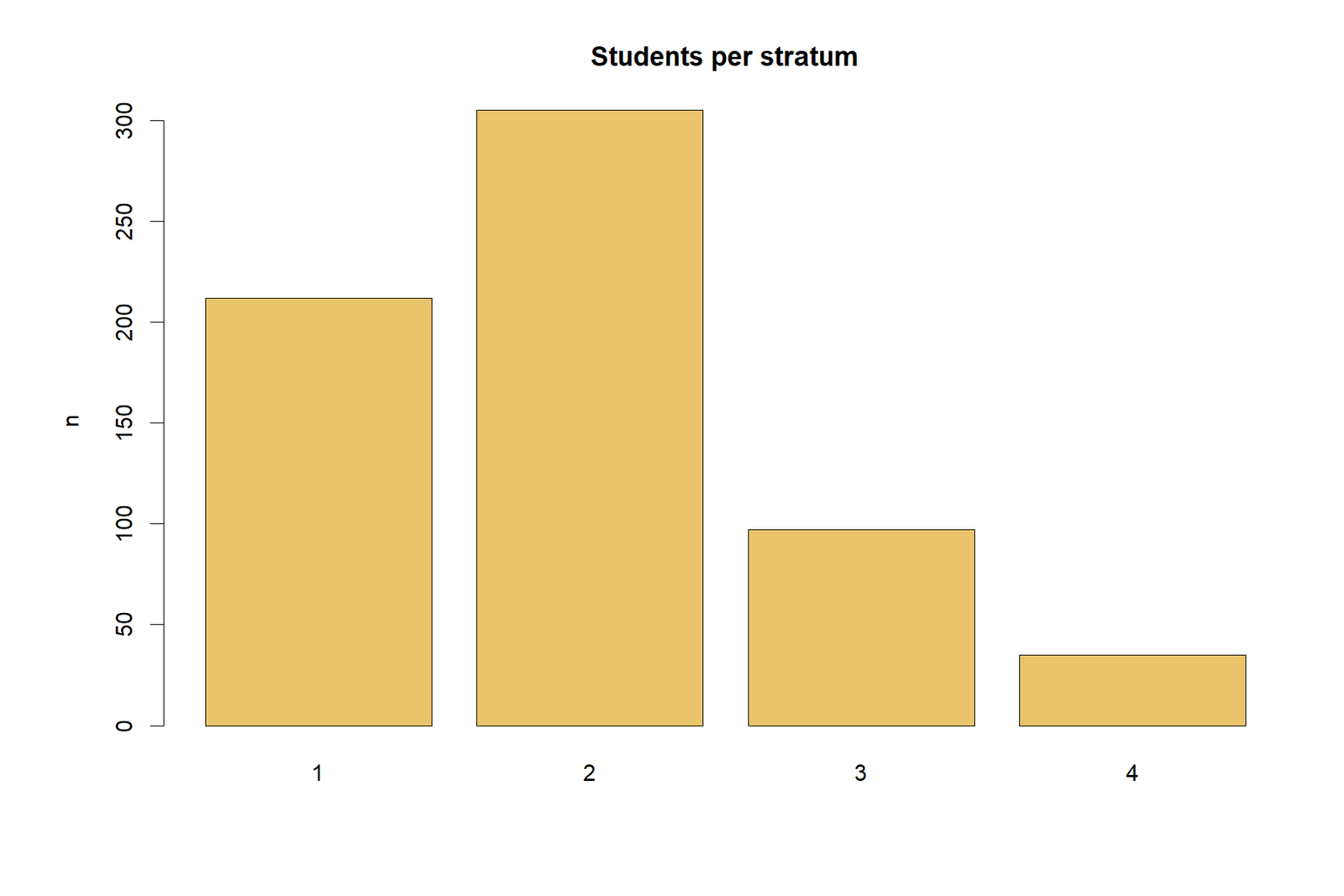
Stratum Sizes
Pattern: Study-time level 2 contains nearly half the sample, while level 4 contains only 35 students.
Interpretation: Unequal sizes cause unequal precision. The small fourth stratum explains its wide confidence interval and sensitivity to the zero cell.
Next step: Include stratum sizes in every heterogeneity report.
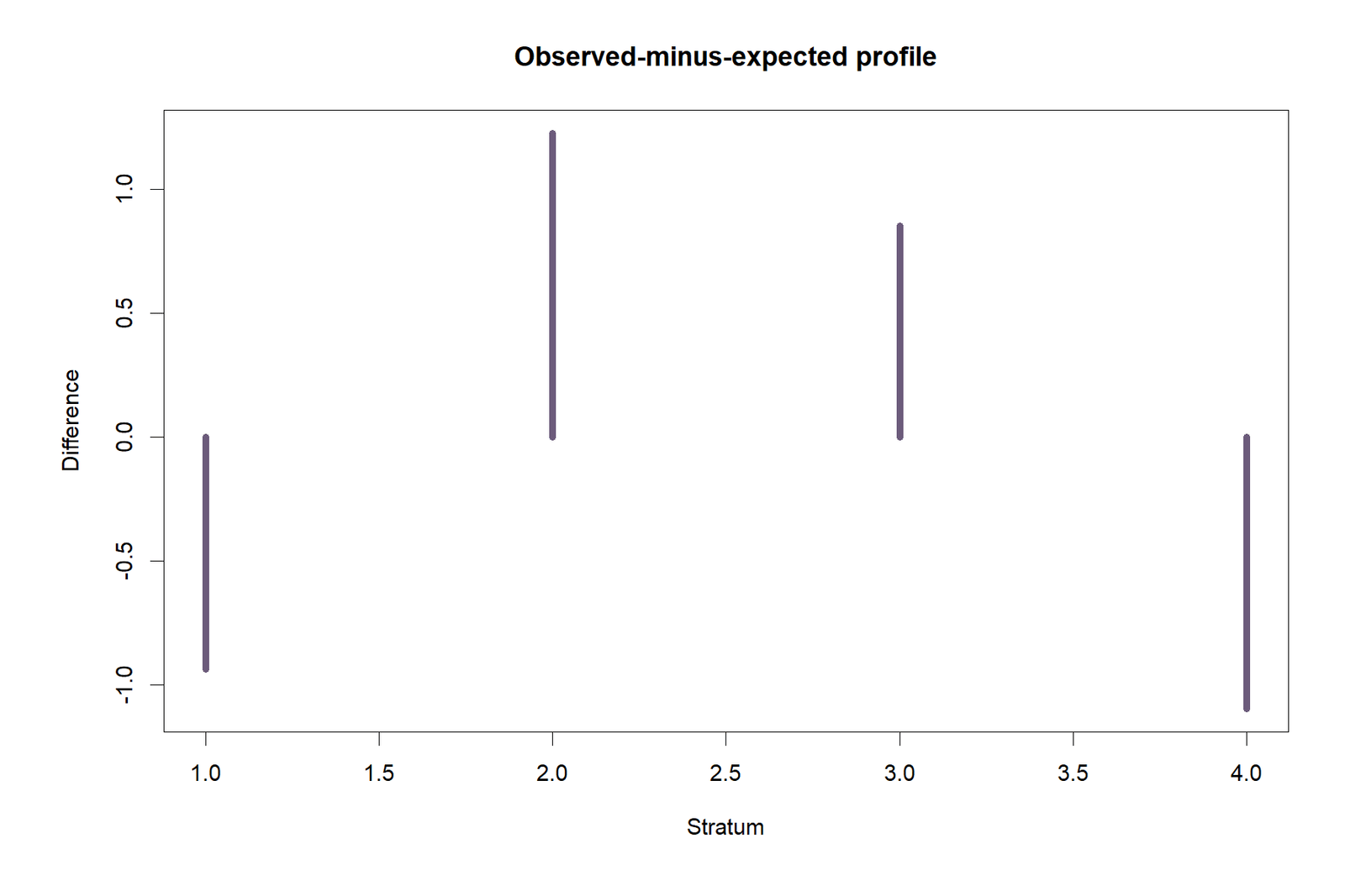
Observed-Minus-Expected Profile
Pattern: Strata 1 and 4 are below expectation; strata 2 and 3 are above expectation.
Interpretation: Positive and negative deviations partly balance. The Tarone adjustment accounts for a small aggregate component of this pattern.
Next step: Use the contribution chart to determine which deviations are large relative to variance.
R Result Summary
Pattern: The result-summary image reproduces the same statistic, p-value and adjustment values used in the worked report.
Interpretation: The R output independently supports the conclusion that odds-ratio heterogeneity was not detected.
Next step: Keep the R and Python sections separate in the public article.
Breslow-Day Test Assumptions, Diagnostics and Limitations
Table Structure
Every stratum must contain the same binary exposure and binary outcome orientation. Strata must be mutually exclusive.
Independence
Observations should be independent within and between strata. Repeated or clustered data require another model.
Approximation Quality
The chi-square reference works best when the strata contain adequate information. Sparse and zero cells require caution.
Independent observations within and between strata
Each student contributes one record to one study-time stratum. If students are clustered within schools or classrooms, conventional standard errors and p-values may not fully reflect the dependence. A generalized estimating equation or multilevel logistic model may be more appropriate for population inference.
Consistent 2 × 2 orientation
Male/female rows and pass/fail columns must remain in the same order in all four tables. Reversing only one stratum creates artificial heterogeneity. Table orientation should be printed beside the results.
Meaningful and prespecified strata
Study-time levels should represent scientifically interpretable groups. Arbitrary data-driven cutpoints can manufacture apparent interaction and reduce power.
Zero cells
The female-fail cell in study-time level 4 is zero. The raw stratum odds ratio is therefore zero. A 0.5 correction is used only for the plotted estimate and interval. The zero cell should be disclosed because it drives instability.
Sparse-stratum influence
Stratum 4 contributes about 75.1% of the homogeneity statistic despite containing only 35 students. This is not a reason to delete it automatically. It is a reason to report sensitivity and interpret the test with the stratum table visible.
Enough strata for interaction detection
With four strata, the test has three degrees of freedom. Moderate departures may be difficult to detect when the smaller strata are imprecise. A nonsignificant result can reflect genuine homogeneity, limited power, or both.
Common odds ratio is scientifically meaningful
Even when homogeneity is not rejected, one pooled effect should be used only when the strata represent settings across which a common odds ratio makes sense. Statistical compatibility is necessary but not always sufficient.
Odds ratio is the intended effect scale
Homogeneity on the odds-ratio scale does not imply homogeneity of risk ratios or risk differences. Effect modification can depend on the chosen scale.
No unmeasured confounding within strata
The test evaluates observed table heterogeneity. It does not control all confounding and cannot establish causation. Additional variables may require binary logistic regression.
Pass threshold and information loss
G3 is originally quantitative. Recoding G3 ≥ 10 produces a useful pass/fail outcome but discards differences among passing and failing grades. The threshold should be justified.
Breslow-Day Test in Python, R, SPSS and Excel
Breslow-Day Test in Python
Python's stratified contingency-table workflow accepts a 2 × 2 × H array. The homogeneity method returns the Breslow-Day Test chi-square statistic and p-value; an adjustment option returns the Tarone result.
- Build tables with identical row and column orientation.
- Use a stratified-table object.
- Run the equal-odds test without and with adjustment.
- Retrieve the pooled odds ratio and confidence interval.
- Print stratum tables and sizes for auditability.
Expected output: BD = 3.441983431; p = 0.328364995; Tarone = 3.441858707.
Breslow-Day Test in R
R can calculate the test through a validated stratified-table package or by reproducing the expected-cell formula. A complete R workflow should report the ordinary statistic, Tarone adjustment, common odds ratio, stratum-specific estimates and zero-cell handling.
- Create a 2 × 2 × 4 array.
- Use one exposure/outcome orientation throughout.
- Request both ordinary and Tarone-adjusted tests.
- Calculate stratum odds ratios with disclosed corrections.
- Save separate R charts and explanations.
Breslow-Day Test in SPSS
SPSS CROSSTABS can produce stratified 2 × 2 tables, risk estimates, CMH statistics, and homogeneity tests when the appropriate statistics are requested. The output should be checked to ensure that the reported Breslow-Day Test test concerns odds-ratio homogeneity rather than a survival-analysis test with a similar name.
- Code sex and pass as binary variables.
- Use studytime as the layer variable.
- Request CMH, risk and cell diagnostics.
- Report Breslow-Day Test and Tarone statistics.
- Retain the full stratum tables in the output.
Breslow-Day Test in Excel
The worked workbook contains six sheets: Guide, Data_Input, Observed_Tables, Calculations, Diagnostics and Reporting. Formula cells reconstruct the common odds ratio, expected cell values, variances, contributions, p-value and Tarone statistic.
- Use COUNTIFS to build the four tables.
- Calculate the common odds ratio from stratum components.
- Solve the expected-cell quadratic.
- Sum standardized contributions.
- Use CHISQ.DIST.RT for the p-value.
The workbook result matches the verified reference to numerical precision.
Cross-Software Values to Preserve
Expandable Breslow-Day Test Code
Python: statsmodels stratified table
import numpy as np
from statsmodels.stats.contingency_tables import StratifiedTable

tables = np.array([
    [[91, 32], [71, 18]],
    [[92, 15], [172, 26]],
    [[21,  1], [69,  6]],
    [[12,  2], [21,  0]],
]).transpose(1, 2, 0)

model = StratifiedTable(tables)

bd = model.test_equal_odds(adjust=False)
tarone = model.test_equal_odds(adjust=True)

print("Breslow-Day Test:", bd.statistic, bd.pvalue)
print("Tarone:", tarone.statistic, tarone.pvalue)
print("Common OR:", model.oddsratio_pooled)
print("Common OR CI:", model.oddsratio_pooled_confint())
print("Common OR=1 test:", model.test_null_odds())
Python: stratum odds ratios with zero-cell display correction
import math

tables = [
    (91, 32, 71, 18),
    (92, 15, 172, 26),
    (21,  1, 69,  6),
    (12,  2, 21,  0),
]

for a, b, c, d in tables:
    raw_or = (a * d) / (b * c) if b * c else math.nan

    # Add 0.5 only for the plotted estimate when any cell is zero.
    if min(a, b, c, d) == 0:
        aa, bb, cc, dd = a + .5, b + .5, c + .5, d + .5
    else:
        aa, bb, cc, dd = a, b, c, d

    plot_or = (aa * dd) / (bb * cc)
    se_log_or = math.sqrt(1/aa + 1/bb + 1/cc + 1/dd)
    lower = math.exp(math.log(plot_or) - 1.96 * se_log_or)
    upper = math.exp(math.log(plot_or) + 1.96 * se_log_or)

    print(raw_or, plot_or, lower, upper)
R: stratified-table workflow
# Example using a validated Breslow-Day Test implementation.
tables <- array(
  c(
    91, 71, 32, 18,
    92, 172, 15, 26,
    21, 69, 1, 6,
    12, 21, 2, 0
  ),
  dim = c(2, 2, 4),
  dimnames = list(
    Sex = c("Male", "Female"),
    Outcome = c("Pass", "Fail"),
    StudyTime = paste0("Level_", 1:4)
  )
)

# Package syntax differs. The chosen function should return:
# Breslow-Day Test chi-square, df, p-value,
# Tarone-adjusted statistic, and common odds ratio.

print(tables)
Confirm the array orientation against printed 2 × 2 tables before interpreting the result.
SPSS: stratified crosstabs
* Create pass status.
COMPUTE pass3 = (G3 >= 10).
VALUE LABELS pass3 0 "No / fail" 1 "Yes / pass".

* Create binary sex coding.
RECODE sex ("F"=0) ("M"=1) INTO sex_bin.
VALUE LABELS sex_bin 0 "Female" 1 "Male".
EXECUTE.

* Stratified tables and homogeneity statistics.
CROSSTABS
  /TABLES=sex_bin BY pass3 BY studytime
  /FORMAT=AVALUE TABLES
  /STATISTICS=CHISQ CMH RISK
  /CELLS=COUNT ROW COLUMN EXPECTED RESID SRESID
  /COUNT ROUND CELL.
Excel: central calculation formulas
Common Mantel-Haenszel odds ratio:
=SUM(a_h*d_h/n_h) / SUM(b_h*c_h/n_h)

Breslow-Day Test contribution for stratum h:
=(Observed_a_h-Expected_a_h)^2/Variance_a_h

Breslow-Day Test statistic:
=SUM(all_contribution_cells)

Degrees of freedom:
=Number_of_strata-1

P-value:
=CHISQ.DIST.RT(BD_statistic, Degrees_of_freedom)

Tarone statistic:
=BD_statistic - Tarone_correction_term
Excel: stratum table construction
Male pass:
=COUNTIFS(studytime_range, stratum,
          sex_range, "M",
          pass_range, 1)

Male fail:
=COUNTIFS(studytime_range, stratum,
          sex_range, "M",
          pass_range, 0)

Female pass:
=COUNTIFS(studytime_range, stratum,
          sex_range, "F",
          pass_range, 1)

Female fail:
=COUNTIFS(studytime_range, stratum,
          sex_range, "F",
          pass_range, 0)
Advanced Breslow-Day Test Topics
Effect Modification Versus Confounding
Stratification can address confounding and reveal effect modification, but these are different concepts. Confounding changes the pooled estimate after adjustment; effect modification means that the association genuinely differs across strata. The Breslow-Day Test targets the latter on the odds-ratio scale.
Homogeneity Depends on the Effect Scale
A set of tables can have homogeneous odds ratios but heterogeneous risk differences. Before interpreting the result, specify why odds ratios are the desired effect measure. Public-health readers may also need stratum-specific risks or probabilities.
Power of the Breslow-Day Test
Power increases with total sample size, number of informative strata, balanced cell counts and larger interaction effects. A small zero-cell stratum can look extreme but add limited reliable information. Sample-size planning should use plausible stratum-specific tables, not only an overall N.
The Role of the Fourth Stratum
Study-time level 4 contains only 35 students and has no female failures. It contributes 2.584 of the total 3.442. A sensitivity analysis can describe how the result changes under a correction or model-based interaction analysis, but the stratum should not be silently omitted.
Tarone Adjustment Interpretation
Tarone adjustment addresses a technical calibration issue in the chi-square statistic. It does not change the null hypothesis, effect scale or scientific interpretation. When ordinary and adjusted results agree, report one as primary and the other as a robustness check.
Logistic Interaction Model
A logistic regression with sex, study-time indicators and sex-by-study-time interaction terms provides a flexible alternative. It can estimate each interaction coefficient, test the interaction jointly and add covariates. The Breslow-Day Test remains useful as a transparent table-based analysis.
Ordered Study-Time Levels
The Breslow-Day Test treats the four strata as categories and does not use their order. A regression interaction can test a linear trend in effect modification if a monotonic change across study-time levels is scientifically plausible.
Many Small Strata
When data are divided into many small strata, asymptotic approximations and individual odds ratios can become unstable. Exact conditional methods, penalized regression or model-based smoothing may be preferable.
Simpson's Paradox
A crude odds ratio can differ from stratum-specific associations because the stratifier is unevenly distributed. The Breslow-Day Test does not diagnose Simpson's paradox by itself; it evaluates whether a common stratum-adjusted odds ratio is plausible.
Common Odds Ratio Confidence Interval
The pooled 95% interval [0.510, 1.254] includes 1. This interval concerns the common effect conditional on a homogeneity interpretation. It should not be used as evidence that the stratum-specific effects are homogeneous.
Zero-Cell Alternatives
A continuity correction is simple for plotting, but Firth logistic regression, exact methods or Bayesian models can provide more principled estimation in sparse data. The choice depends on the study aim and available software.
Multiple Potential Effect Modifiers
Testing many stratifiers separately creates multiplicity and can produce inconsistent stories. A prespecified interaction strategy and model-based joint analysis are more defensible than searching every categorical variable.
APA Reporting for the Breslow-Day Test
A complete APA-style report identifies the exposure, outcome, stratifier, number of strata, total sample size, statistic, degrees of freedom, p-value, decision and common-effect context. It also distinguishes homogeneity from the separate test of the common odds ratio.
Full Worked APA Result
A Breslow-Day Test test evaluated whether the male-versus-female odds ratio for passing G3 (G3 ≥ 10) was homogeneous across four study-time strata, N = 649. The homogeneity test was not statistically significant, χ²(3) = 3.44, p = 0.328, indicating insufficient evidence that the stratum-specific odds ratios differed. The Mantel–Haenszel common odds ratio was 0.80, 95% CI [0.51, 1.25], and the separate common-effect test was not significant, χ²(1) = 0.93, p = 0.334.
Concise APA Result
Odds ratios were statistically homogeneous across study-time levels, Breslow-Day Test χ²(3) = 3.44, p = 0.328. The common odds ratio was 0.80, 95% CI [0.51, 1.25].
APA-Style Methods Sentence
Sex-by-pass 2 × 2 tables were formed within four study-time strata, and a Breslow-Day Test chi-square test assessed homogeneity of the stratum-specific odds ratios; a Tarone-adjusted result was calculated as a sensitivity analysis.
APA Results Table
| Measure | Complete value | APA presentation |
|---|---|---|
| Total sample | 649 | N = 649 |
| Number of strata | 4 | 4 study-time strata |
| Breslow-Day Test statistic | 3.441983431 | χ² = 3.44 |
| Degrees of freedom | 3 | df = 3 |
| P-value | 0.328364995 | p = 0.328 |
| Tarone statistic | 3.441858707 | χ² = 3.44 |
| Tarone p-value | 0.328381509 | p = 0.328 |
| Common odds ratio | 0.799911650 | OR = 0.80 |
| Common OR interval | [0.510177046, 1.254189409] | 95% CI [0.51, 1.25] |
Reusable APA Templates
Homogeneous Odds Ratios
Exposure and outcome were analysed across H strata.
The Breslow-Day Test was not significant, χ²(df) = statistic, p = p-value.
There was insufficient evidence that the stratum-specific odds ratios differed. The common OR was estimate, 95% CI [lower, upper].
Do not write that homogeneity was proved.
Heterogeneous Odds Ratios
The exposure–outcome association was compared across H strata.
The Breslow-Day Test indicated heterogeneity, χ²(df) = statistic, p = p-value.
Stratum-specific odds ratios ranged from minimum to maximum, with the largest contribution from stratum.
Avoid presenting one pooled odds ratio as the only effect.
Tarone-Adjusted Sensitivity Report
The ordinary Breslow-Day Test result was χ²(df) = statistic, p = p-value.
The Tarone-adjusted result was χ²(df) = adjusted statistic, p = adjusted p-value.
The adjustment did/did not change the substantive conclusion.
Identify Tarone as an adjustment, not a different research hypothesis.
APA Language Rules
| Avoid | Use instead | Reason |
|---|---|---|
| The odds ratios were equal. | No statistically significant heterogeneity was detected. | Nonsignificance does not prove equality. |
| The Breslow-Day Test showed no association. | The test did not detect variation in the association across strata. | Homogeneity and association are different questions. |
| OR = 0 in stratum 4 without explanation. | State the zero cell and any correction used for display. | Zero-cell estimates are unstable. |
| p = .328, therefore use one pooled effect automatically. | Use a pooled effect when homogeneity and scientific meaning support it. | Statistical compatibility is not the only criterion. |
Common Mistakes and Final Reporting Checklist
Common Mistakes
| Mistake | Correction |
|---|---|
| Calling it a test of association | Describe it as a test of odds-ratio homogeneity. |
| Using inconsistent table orientation | Keep exposure and outcome coding identical in all strata. |
| Ignoring sparse and zero cells | Report them and explain any correction. |
| Reporting only point estimates | Add confidence intervals, stratum sizes and contributions. |
| Using a pooled OR after significant heterogeneity | Emphasize stratum-specific effects or interaction modelling. |
| Interpreting p > .05 as proof | Use “insufficient evidence of heterogeneity.” |
| Confusing Tarone with survival-analysis Tarone-Ware | Name the odds-ratio homogeneity adjustment precisely. |
| Deleting the influential small stratum | Use transparent sensitivity analysis. |
Publication Checklist
- State the binary exposure and outcome coding.
- Name the stratifying variable and all levels.
- Show every 2 × 2 table and stratum N.
- Report stratum-specific odds ratios and intervals.
- Report χ², df and p for the Breslow-Day Test.
- State whether Tarone adjustment was used.
- Separate homogeneity from the common-effect test.
- Explain zero-cell handling.
- Report the common OR only with appropriate context.
- Keep Python and R charts in separate sections.
Breslow-Day Test Reports and Worked Excel Download
R Result Summary ImagePublished R summary graphic showing the ordinary and Tarone-adjusted results.
SPSS Breslow-Day Test OutputStratified crosstabs, risk estimates, CMH context and supporting SPSS output.
Worked Breslow-Day Test Excel WorkbookEditable data, observed tables, calculations, diagnostics and reporting sheets.
Frequently Asked Questions About the Breslow-Day Test
What is the Breslow-Day Test?
It is a chi-square test of whether odds ratios are homogeneous across a set of stratified 2 × 2 contingency tables.
What is the null hypothesis?
All stratum-specific odds ratios equal one common odds ratio.
What is the alternative hypothesis?
At least one stratum-specific odds ratio differs from the others.
What is the worked statistic?
The verified Breslow-Day Test statistic is 3.441983431.
What are the degrees of freedom?
With four strata, df = H − 1 = 3.
What is the p-value?
The verified p-value is 0.328364995, reported as .328.
Was heterogeneity significant?
No. The test did not reject homogeneity at alpha .05.
Does a nonsignificant result prove equal odds ratios?
No. It means the available data did not provide sufficient evidence of heterogeneity.
What is the Tarone-adjusted result?
The adjusted statistic is 3.441858707 and p = 0.328381509.
What is the common odds ratio?
The Mantel–Haenszel common odds ratio is 0.799911650.
What is its confidence interval?
The 95% confidence interval is [0.510177, 1.254189].
Is the common odds ratio significant?
No. The separate common-effect test gives p = 0.334.
What is the difference between Breslow-Day Test and CMH?
Breslow-Day Test tests effect homogeneity; CMH tests or estimates a common stratified association.
How many strata are analysed?
Four study-time strata are analysed.
What are the stratum sample sizes?
The stratum sizes are 212, 305, 97 and 35.
Which stratum contributes most to heterogeneity?
Study-time level 4 contributes 2.5835, about 75% of the total statistic.
Why is stratum 4 unstable?
It contains only 35 students and has a zero female-fail cell.
What is the raw odds ratio in stratum 4?
The raw cross-product odds ratio is 0 because one cell is zero.
Why does the chart show 0.116 for stratum 4?
The plotted estimate uses a 0.5 continuity correction to obtain a finite log odds ratio and interval.
Does continuity correction change the primary test?
The correction is disclosed for the chart. The validated homogeneity workflow uses its specified raw-table calculation.
Can the test be used for risk ratios?
The standard Breslow-Day Test concerns odds-ratio homogeneity, not risk-ratio or risk-difference homogeneity.
Can it be used for more than four strata?
Yes. The method supports H strata, with nominal df = H − 1.
Can it be used with paired observations?
No. Standard stratified tables assume independent observations.
Can it test a continuous effect modifier?
Not directly. Logistic regression interaction is generally preferable for continuous modifiers.
How is the test run in Python?
Use a stratified 2 × 2 table object and its equal-odds test, with the adjustment option for Tarone.
How is the test run in R?
Use a validated stratified-table homogeneity function or reproduce the expected-cell formula.
How is the test run in SPSS?
Use stratified CROSSTABS with CMH, risk and homogeneity statistics, then verify the printed tables and test labels.
Can Excel calculate it?
Yes. The worked workbook calculates the common odds ratio, expected cells, variances, contributions, statistic, p-value and Tarone result.
What should an APA report include?
Include exposure, outcome, stratifier, H, N, chi-square, df, p-value, decision, common OR and interval.
What should be reported after significant heterogeneity?
Report stratum-specific estimates, intervals, influential strata and an interaction analysis rather than relying on one pooled effect.
What should be reported after nonsignificant heterogeneity?
State that heterogeneity was not detected, then report a common effect only when scientifically appropriate.
What is the main conclusion here?
No significant variation in the sex–pass odds ratio was detected across study-time strata, and the common odds ratio was also not significantly different from 1.
Breslow-Day Test Conclusion
Statistical Conclusion
The verified Breslow-Day Test produced χ²(3) = 3.441983, p = 0.328365. The Tarone-adjusted result was essentially identical. The analysis therefore found insufficient evidence that the male-versus-female pass odds ratio varied across the four study-time strata.
Substantive Conclusion
A common odds ratio of 0.800 can be used as a descriptive stratified summary, but its 95% interval [0.510, 1.254] includes 1 and the separate common-effect p-value is 0.334. The data do not establish either effect modification or a common sex effect on pass odds.
The small fourth stratum creates the largest heterogeneity contribution and should remain visible in the report. Its zero cell explains the corrected chart estimate and wide interval. The correct public interpretation is not that all odds ratios are exactly equal, but that the observed differences are compatible with sampling variation under the common-odds model.

