Zero Inflated Negative Binomial Regression: Formula, Results, Python, R, SPSS and Excel
Zero Inflated Negative Binomial Regression separates a latent structural-zero process from an overdispersed count process that can also generate zero. This complete 649-case guide connects the two formulas with alpha, IRRs, inflation odds ratios, zero calibration, residual error, model comparison and reproducible software workflows.
Zero Inflated Negative Binomial Regression Model Overview
Zero Inflated Negative Binomial Regression is designed for nonnegative count outcomes that show both more zeros and more positive-count variation than a simple Poisson process can represent adequately. The worked outcome is student absences for 649 records. It contains 244 zeros, 405 positive counts, a mean of 3.659476 and observed values from 0 through 32.
The model contains two linked equations. The negative-binomial count component uses G1, G2, G3, age, studytime, failures, school and sex. The inflation component uses failures, studytime, G1, G2 and G3 to estimate the probability of membership in a latent excess-zero state. These components share one outcome but have different scales and interpretations.
Every observed zero is ambiguous. A structural zero is generated by the inflation state. A sampling zero is produced naturally by the NB2 count state. Zero Inflated Negative Binomial Regression estimates the probability of each mechanism; it does not observe or prove the source of an individual zero.
The count equation uses a log link and exponentiated coefficients are incidence rate ratios. The inflation equation uses a logit link and exponentiated coefficients are structural-zero odds ratios. An IRR and an inflation odds ratio must never be described as the same effect.
The NB2 count variance is mu plus alpha multiplied by mu squared. Alpha is estimated as 0.383057 with SE 0.051533, z = 7.4333 and p approximately 1.06 × 10⁻¹³. This supports substantial overdispersion relative to a Poisson count state.
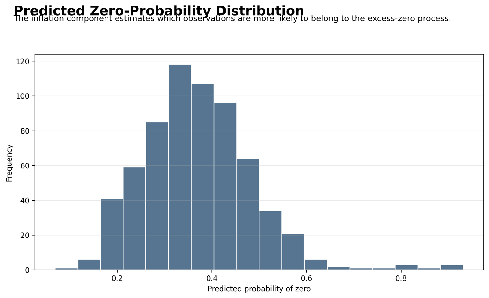
The direct fit converged at log likelihood −1451.811111, AIC 2935.622221 and conventional BIC 3007.229145. The model predicts 241.138886 zeros and a mean zero probability of 0.371555, close to the observed zero rate of 0.375963.
The benefits of Zero Inflated Negative Binomial Regression are flexible overdispersion, separate process interpretation and direct zero-probability prediction. Its limitations include latent-state ambiguity, possible weak identification, sensitivity to component specification, complex cross-software parameterizations and the absence of ordinary one-equation effect summaries.
Quick Answer
The verified Zero Inflated Negative Binomial Regression fit converges and estimates both an excess-zero process and an overdispersed NB2 count process.
What the output supports
- The direct mixture fits the observed zero rate closely.
- NB2 overdispersion is clearly different from the Poisson boundary.
- ZINB AIC is 139.57 below the ordinary NB comparison.
- G1 and G3 contribute to the inflation equation.
- G3, age, studytime and school contribute to the count equation.
What it does not prove
- It does not identify which individual zeros are structural.
- It does not establish causal predictor effects.
- It does not guarantee accurate individual absence prediction.
- It does not validate the model in a new sample.
- It does not make the two component coefficients directly comparable.
Table of Contents
- Model Overview
- Quick Answer
- Why the Model Is Needed
- How the Mixture Works
- Variables and Coding
- Verified Results
- Python Chart Stories
- R Chart Pairs
- Coefficient Interpretation
- Predictions and Meaning
- Assumptions and Diagnostics
- Python, R, SPSS and Excel
- Code and Formulas
- Advanced Topics
- APA-Style Reporting
- Publication Checklist
- Downloads
- Related Guides
- Frequently Asked Questions
- Conclusion
Why This Analysis Needs Zero Inflated Negative Binomial Regression
The absence outcome combines three features: a boundary mass of 244 zeros, a long right tail through 32 and positive-count variation that exceeds a Poisson mean-variance restriction. A one-process Poisson equation cannot represent all three features comfortably.
An ordinary negative-binomial model addresses overdispersion, but it treats every zero as a possible realization from the same count process. Zero Inflated Negative Binomial Regression adds a second latent route to zero and asks whether a mixture improves fit and calibration.
The candidate comparison supports the mixture. ZINB AIC is 2935.622, ordinary NB AIC is 3075.189 and Poisson AIC is 4461.466. The comparison is large enough to justify careful mixture interpretation, but information criteria do not replace residual or process checks.
How Zero Inflated Negative Binomial Regression Works
NB2 Count Equation
The exponential link keeps mu positive. Exponentiating a numeric count slope gives the multiplicative rate change for a one-standard-deviation predictor increase because the supplied numerical predictors are standardized.
Inflation Equation
Pi is the probability of the structural-zero state. Exponentiating gamma gives an odds ratio for that latent state. A lower structural-zero probability can increase the unconditional expected count even when the count-state mean is unchanged.
Mixture Probability
Positive counts can only arise from the NB2 state. Zeros can arise from either state. The likelihood sums the two zero pathways and estimates both coefficient vectors and alpha jointly.
Four-Step Workflow
Variables Used, Coding and Standardization
The same design must be preserved when reproducing Zero Inflated Negative Binomial Regression across software.
| Role | Variable | Coding | Component and interpretation |
|---|---|---|---|
| Outcome | absences | Nonnegative integer count, 0–32 | Observed response; 244 zeros and 405 positive counts |
| Numeric predictor | G1 | Population-SD standardized | Count and inflation components |
| Numeric predictor | G2 | Population-SD standardized | Count and inflation components |
| Numeric predictor | G3 | Population-SD standardized | Count and inflation components |
| Numeric predictor | age | Population-SD standardized | Count component only |
| Numeric predictor | studytime | Population-SD standardized | Count and inflation components |
| Numeric predictor | failures | Population-SD standardized | Count and inflation components |
| Categorical predictor | school_MS | 1 = MS; reference = GP | Count-state rate comparison |
| Categorical predictor | sex_M | 1 = male; reference = female | Count-state rate comparison |
The inflation formula excludes age, school and sex. This is a modeling choice, not evidence that those variables cannot affect zero risk. Changing either formula creates a different mixture and can change every coefficient.
Verified Zero Inflated Negative Binomial Regression Results
Model Comparison
| Model | N | Log likelihood | Parameters inferred from AIC | AIC | Conventional BIC |
|---|---|---|---|---|---|
| Zero Inflated Negative Binomial Regression | 649 | −1451.811111 | 16 | 2935.622221 | 3007.229145 |
| Negative binomial GLM comparison | 649 | −1528.594344 | 9 | 3075.188687 | 3115.467582 |
| Poisson GLM comparison | 649 | −2221.732760 | 9 | 4461.465520 | 4501.744414 |
The source comparison CSV contains invalid negative BIC values for the Poisson and NB rows. The conventional values above are transparently recalculated as −2 log likelihood plus k log(649), using k implied by each supplied AIC.
Calibration and Error
| Measure | Exact value | Interpretation |
|---|---|---|
| Observed zeros | 244 | 37.5963% of 649 observations |
| Expected zeros | 241.138886 | Only 2.861 cases below the observed total |
| Mean predicted probability of zero | 0.371555 | Close to observed zero rate 0.375963 |
| Observed mean | 3.659476 | Average recorded absences |
| Fitted mean | 3.626376 | Mean difference equals 0.033100 |
| MAE | 3.209610 | Average absolute fitted-sample error |
| RMSE | 4.372941 | Larger errors receive extra weight |
| Observed-fitted correlation | 0.333532 | Modest case-level agreement |
| Pearson residual SD | 2.222731 | Substantial residual dispersion remains |
Count, Inflation and Dispersion Parameters
| Component | Term | B | SE | z | p | IRR / OR | 95% effect interval |
|---|---|---|---|---|---|---|---|
| Inflation | Intercept | -0.767284 | 0.107753 | -7.1208 | < .001 | 0.464272 | 0.375884–0.573446 |
| Inflation | failures | -0.103254 | 0.118435 | -0.8718 | 0.3833 | 0.901898 | 0.715065–1.137547 |
| Inflation | studytime | 0.100755 | 0.097829 | 1.0299 | 0.3031 | 1.106005 | 0.913030–1.339768 |
| Inflation | G1 | 0.722911 | 0.211160 | 3.4235 | 0.000618 | 2.060422 | 1.362122–3.116709 |
| Inflation | G2 | 0.587383 | 0.308247 | 1.9056 | 0.056707 | 1.799274 | 0.983371–3.292134 |
| Inflation | G3 | -1.199572 | 0.305050 | -3.9324 | 0.000084 | 0.301323 | 0.165719–0.547888 |
| Count | Intercept | 1.814182 | 0.056935 | 31.8640 | < .001 | 6.136053 | 5.488147–6.860446 |
| Count | G1 | 0.048587 | 0.085322 | 0.5695 | 0.5690 | 1.049787 | 0.888127–1.240873 |
| Count | G2 | 0.075824 | 0.144378 | 0.5252 | 0.5995 | 1.078773 | 0.812897–1.431610 |
| Count | G3 | -0.334885 | 0.156312 | -2.1424 | 0.032160 | 0.715420 | 0.526633–0.971884 |
| Count | age | 0.148952 | 0.041232 | 3.6126 | 0.000303 | 1.160617 | 1.070515–1.258303 |
| Count | studytime | -0.090671 | 0.040917 | -2.2160 | 0.026692 | 0.913318 | 0.842934–0.989579 |
| Count | failures | -0.000905 | 0.041725 | -0.0217 | 0.9827 | 0.999096 | 0.920642–1.084235 |
| Count | school_MS | -0.526762 | 0.091043 | -5.7859 | < .001 | 0.590514 | 0.494009–0.705872 |
| Count | sex_M | 0.004985 | 0.080951 | 0.0616 | 0.9509 | 1.004998 | 0.857551–1.177797 |
| Dispersion | alpha | 0.383057 | 0.051533 | 7.4333 | < .001 | — | 0.282054–0.484061 coefficient CI |
In the count state, age has IRR 1.160617, G3 has IRR 0.715420, studytime has IRR 0.913318 and school_MS has IRR 0.590514, with supplied intervals excluding one. In the inflation state, G1 has OR 2.060422 and G3 has OR 0.301323, with intervals excluding one.
Python Charts and Exact-Value Explanations
Six unique Python figures connect the visible distribution, prediction, residual, effect and comparison evidence with exact Zero Inflated Negative Binomial Regression values.
Python Chart 1: Absence Count Distribution
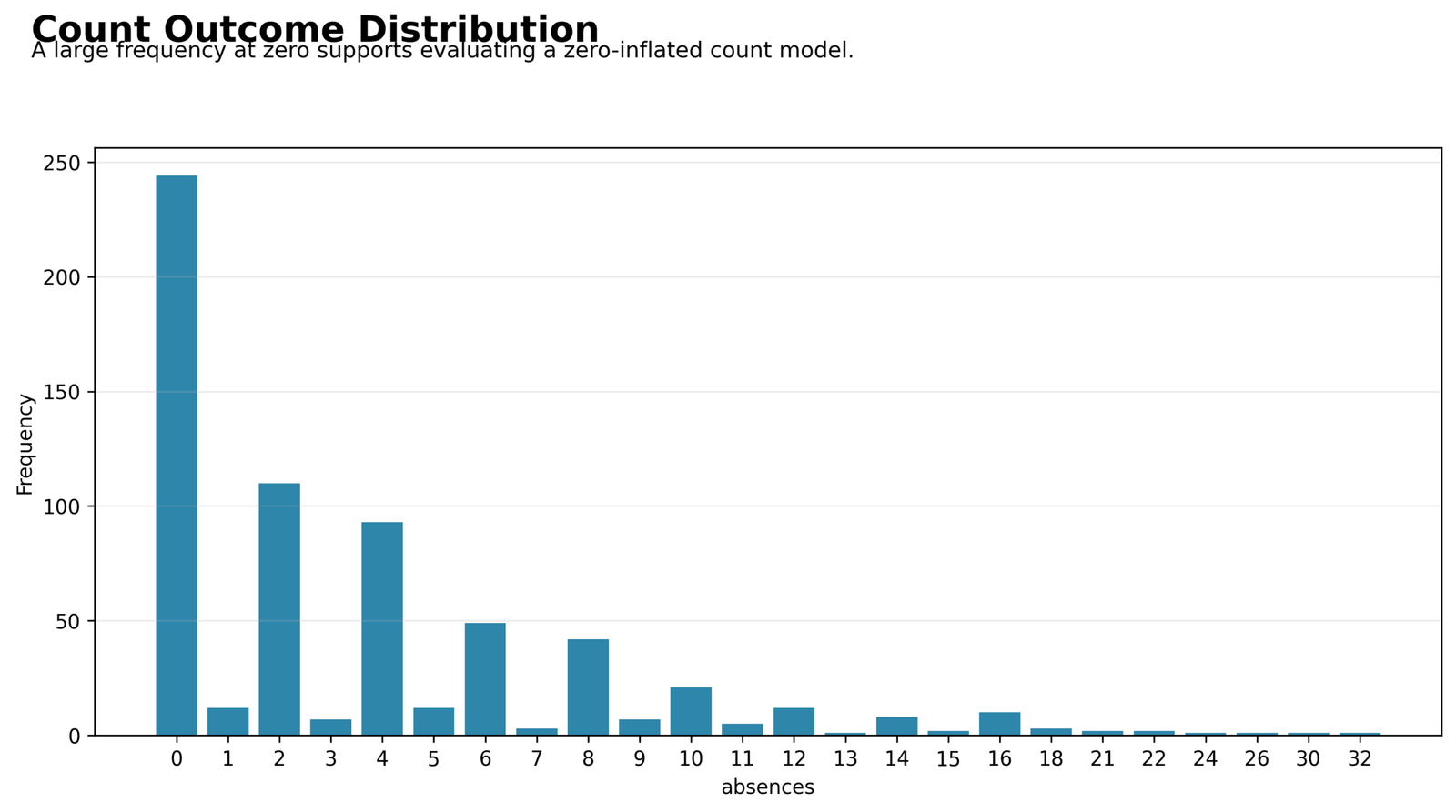
A large zero spike is followed by irregular positive-count peaks and a long right tail.
244 zeros, 405 positive counts, mean 3.659476 and maximum 32.
The shape motivates both an overdispersed count state and investigation of an additional zero process.
The outcome graph establishes the modeling problem before coefficients are interpreted.
Python Chart 2: Observed versus Fitted Counts
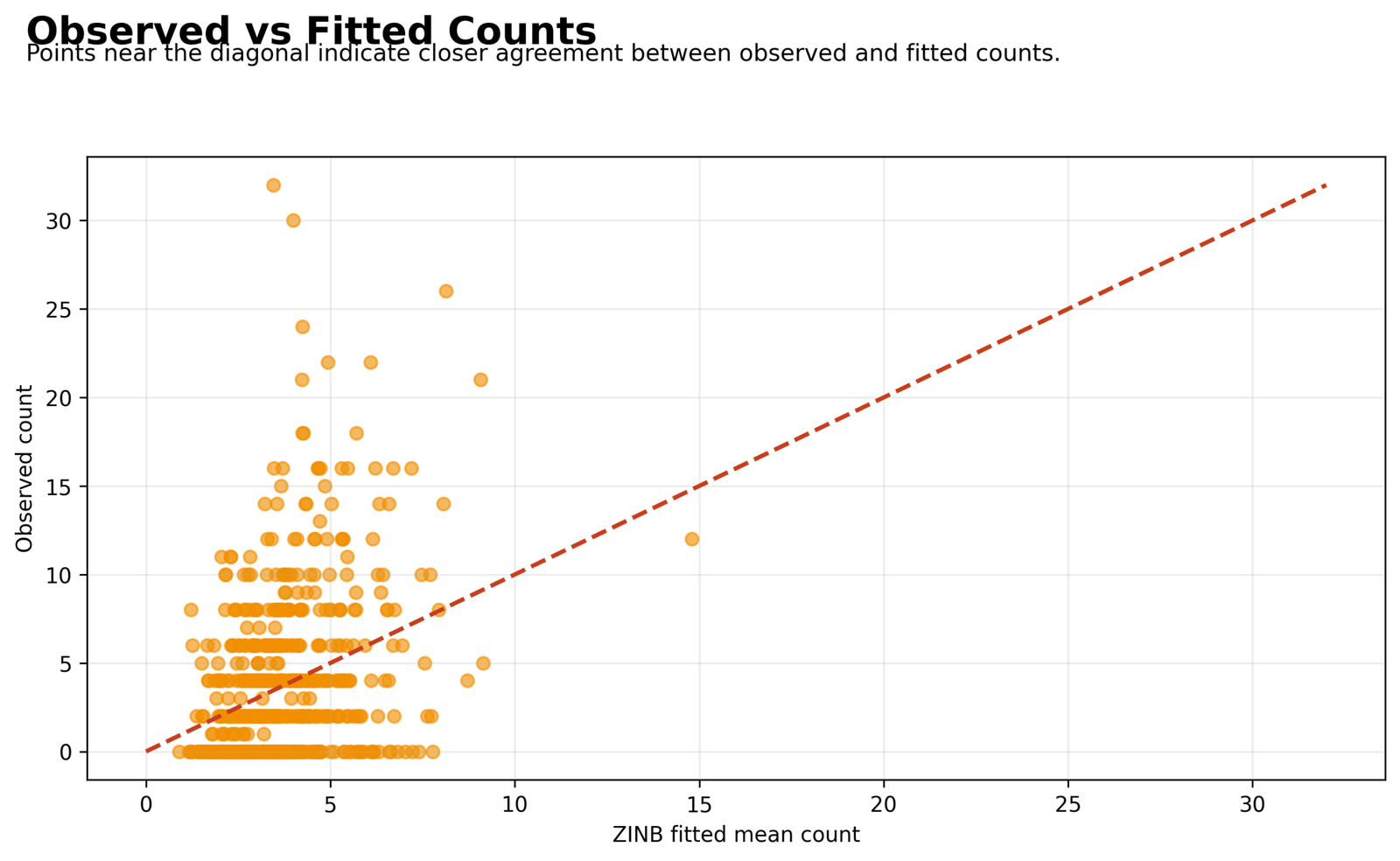
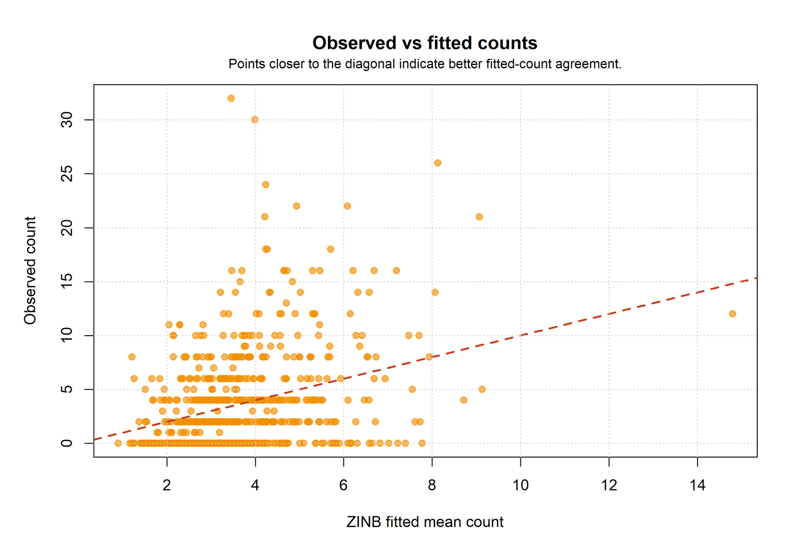
Fitted means occupy a narrower range than the observed right tail, and many large counts lie above their fitted values.
Observed-fitted correlation = 0.333532, MAE = 3.209610 and RMSE = 4.372941.
Good aggregate zero calibration coexists with modest individual count prediction.
The chart prevents AIC superiority from being mistaken for precise case-level forecasting.
Python Chart 3: Pearson Residuals versus Fitted Means
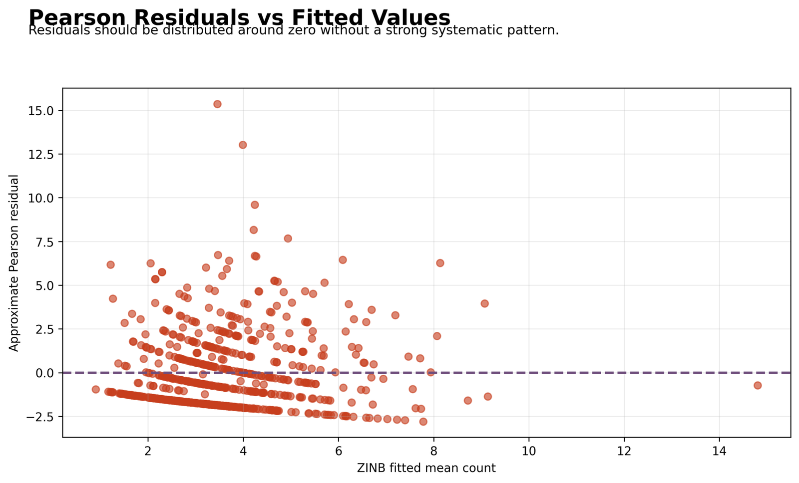
Discrete count bands remain visible, and several positive residuals extend far above the main cloud.
Pearson residual SD = 2.222731 and the upper tail contains very large positive discrepancies.
NB2 dispersion absorbs substantial variability but does not remove all extreme lack of fit.
Exceptional cases and unmodeled structure remain relevant after convergence.
Python Chart 4: Exponentiated Component Effects
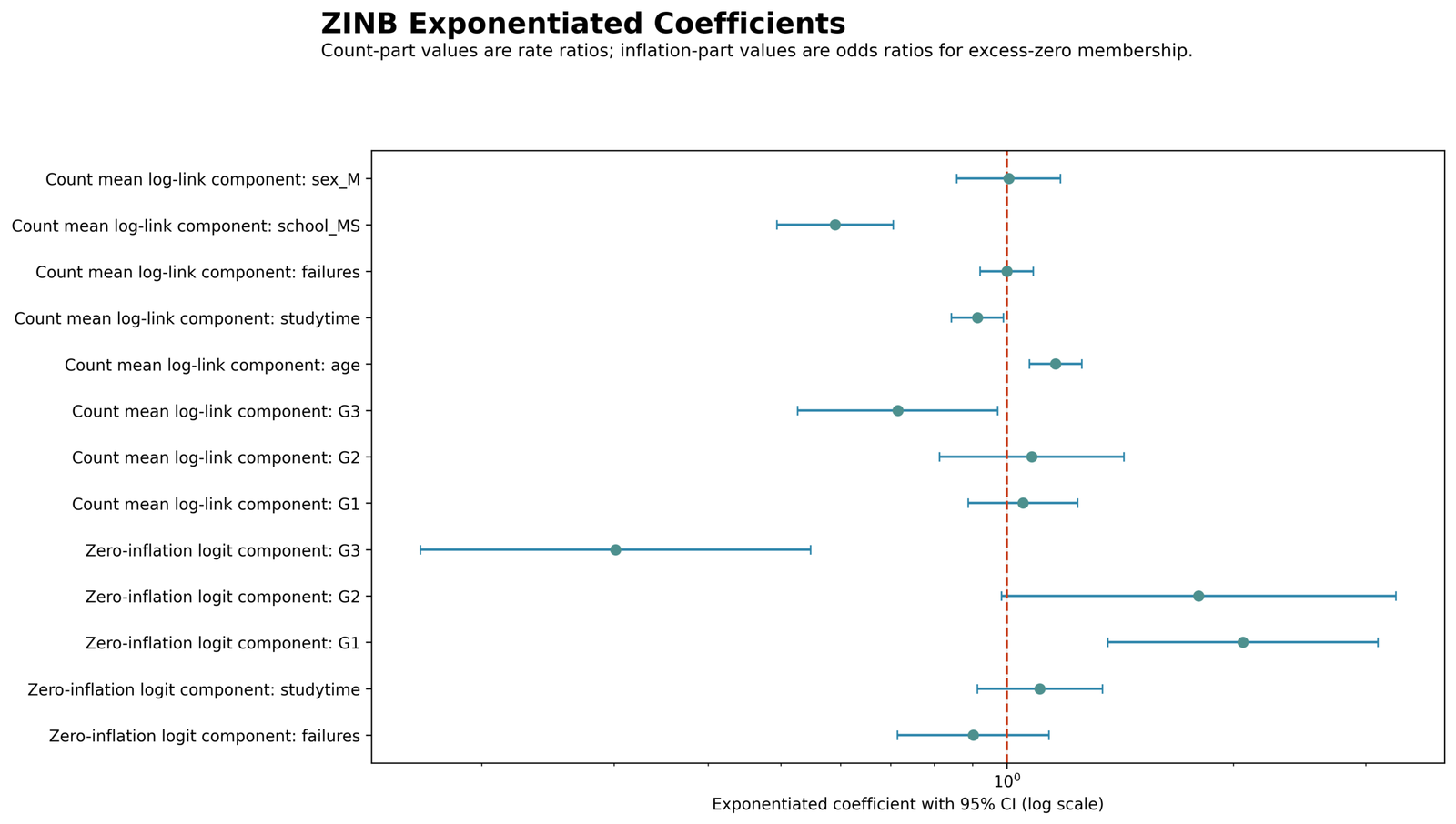
Several intervals exclude one, but count and inflation estimates occupy different estimand families.
Count age IRR = 1.160617; count school_MS IRR = 0.590514; inflation G1 OR = 2.060422; inflation G3 OR = 0.301323.
The common null reference is one, but the effects answer different process questions.
Component labels prevent a structural-zero odds ratio from being described as a count-rate change.
Python Chart 5: Observed and Model-Implied Zero Rates
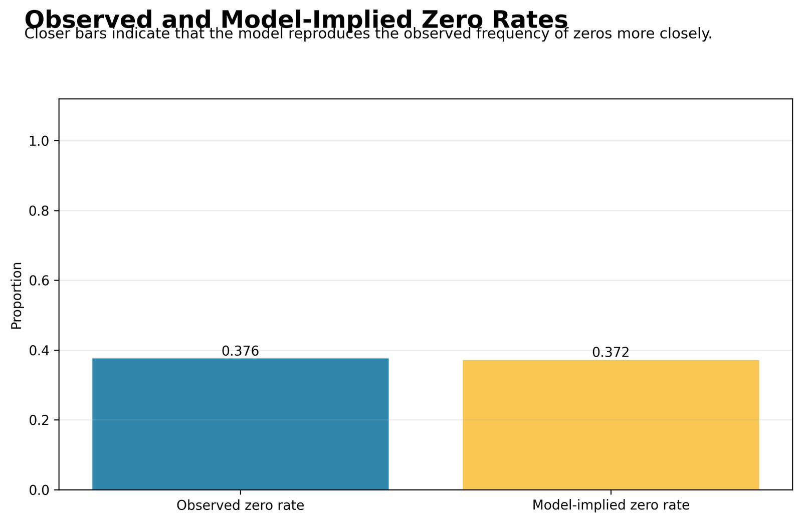
The observed and model-implied zero rates are visually close.
Observed rate = 0.375963; mean predicted P(zero) = 0.371555; expected zeros = 241.138886.
The mixture reproduces the total zero burden closely.
Zero calibration is a core diagnostic that ordinary fitted-count plots can hide.
Python Chart 6: Model Comparison
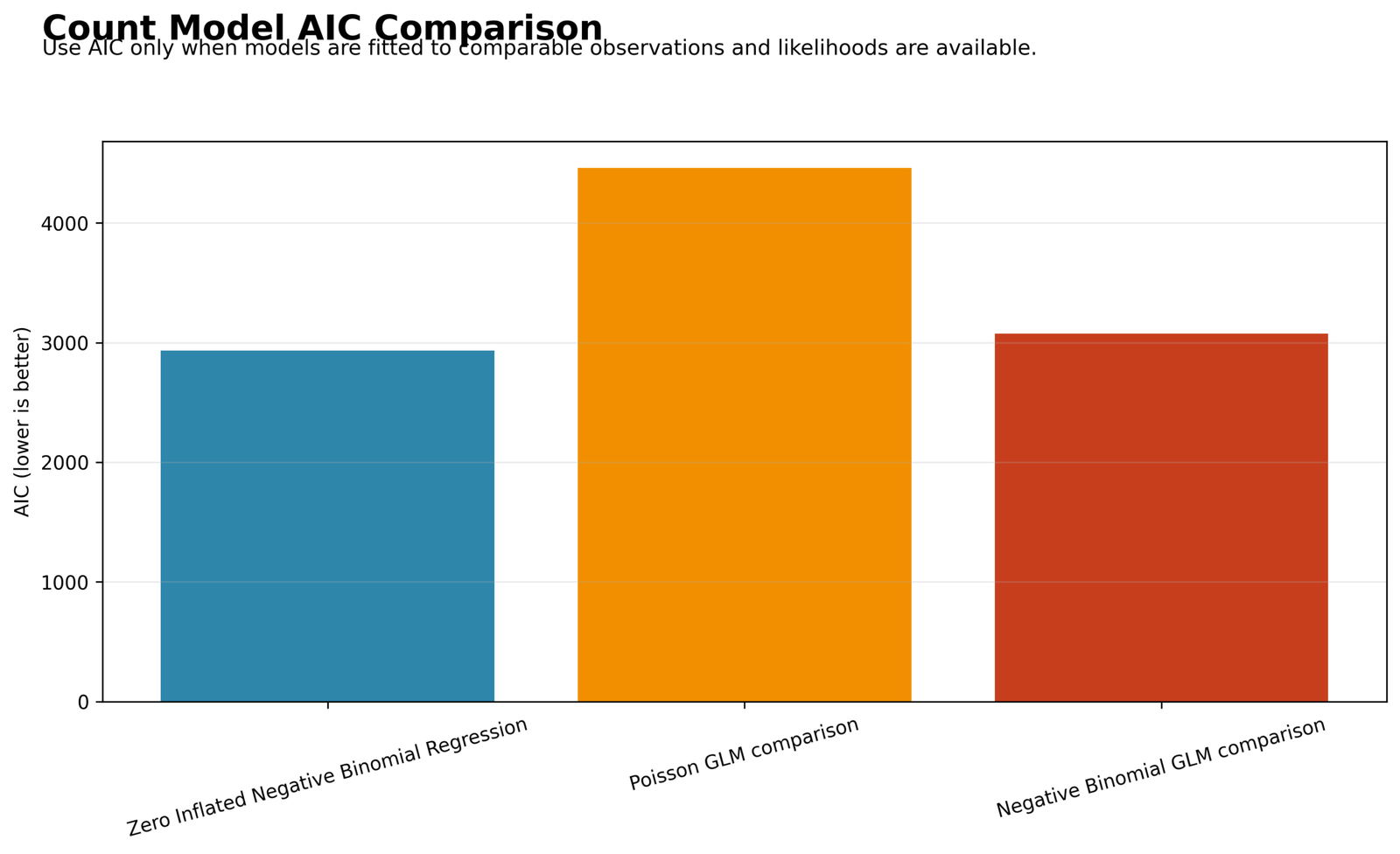
ZINB has the lowest AIC by a wide margin.
ZINB = 2935.622; NB = 3075.189; Poisson = 4461.466.
The mixture provides the best fitted likelihood-complexity balance among these candidates.
The comparison supports the extra zero process while leaving process plausibility and validation as separate questions.
R Charts and Paired Explanations
The attachment supplies four R-labeled visual assets and an R code excerpt, but its own FAQ states that no completed R output exists. The figures are therefore presented as companion reproduction visuals, not as verified independent numerical estimation.
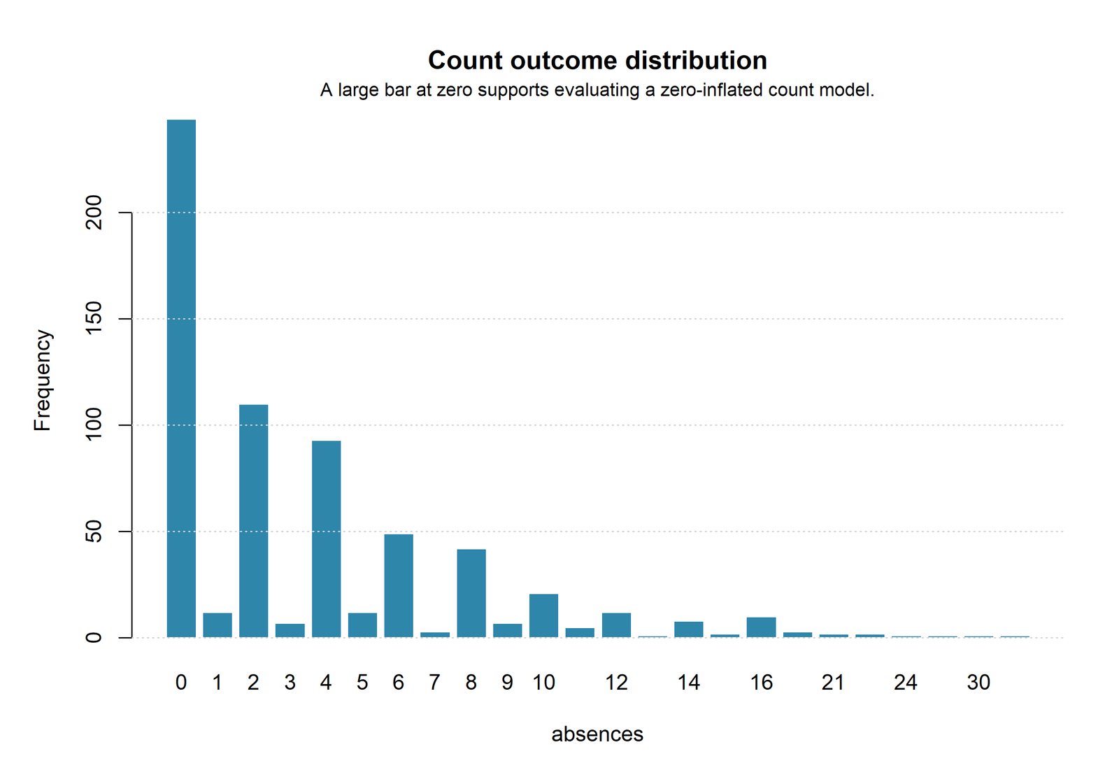
R Chart 1: Outcome Distribution
Pattern: The same zero spike and right tail should appear when R reads the identical 649 rows.
Key values: 244 zeros, mean 3.659476 and maximum 32.
Interpretation: Distribution agreement checks data preparation, not model equality.
R Chart 2: Fitted Count Pattern
Pattern: Large observed counts remain difficult to reproduce from moderate fitted means.
Key values: Python correlation = 0.333532, MAE = 3.209610 and RMSE = 4.372941.
Interpretation: A completed R fit should be compared only after formula, standardization and alpha conventions match.
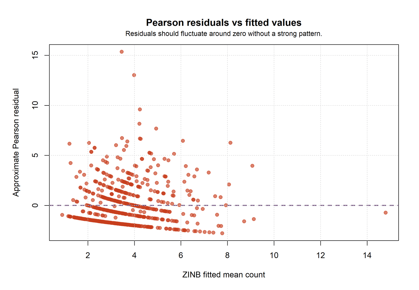
R Chart 3: Residual Pattern
Pattern: Discrete bands and extreme positive residuals remain visible.
Key values: Python Pearson residual SD = 2.222731.
Interpretation: A completed R residual definition must be documented before exact comparison.
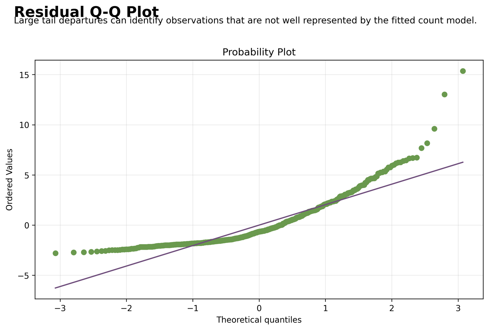
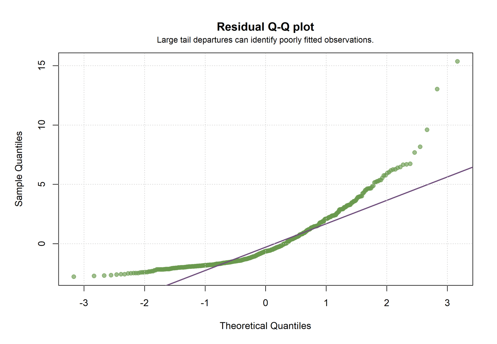
R Chart 4: Residual Tails
Pattern: Strong tail departures identify difficult observations rather than a formal normality requirement.
Key values: The source describes an S-shaped pattern and a pronounced upper tail.
Interpretation: Count residual Q-Q plots are exploratory diagnostics.
Zero Inflated Negative Binomial Regression Coefficient and Parameter Interpretation
Count-State Effects
Age has B = 0.148952 and IRR = 1.160617. Holding the other count predictors fixed, a one-standard-deviation age increase is associated with a 16.06% higher expected absence count inside the count-generating state.
G3 has IRR = 0.715420, studytime has IRR = 0.913318 and school_MS has IRR = 0.590514. Their supplied intervals exclude one. The school result compares MS with the GP reference category. It does not represent a standardized numeric change.
G1, G2, failures and sex_M have count-state intervals crossing one. Their estimates remain part of the declared count formula, but the source uncertainty does not support a conventional nonzero claim at 0.05.
Inflation-State Effects
G1 has B = 0.722911 and structural-zero OR = 2.060422. G3 has B = −1.199572 and OR = 0.301323. These are odds effects for latent excess-zero membership, not changes in the count-state absence rate.
Inflation G2 has OR = 1.799274 with p = 0.056707. failures and studytime also have intervals crossing one. Borderline or uncertain inflation coefficients should not be moved into the count interpretation.
Dispersion
Alpha = 0.383057 is positive and precise. The count-state variance therefore grows quadratically with mu. Software reporting theta or size should be converted through alpha = 1/theta before comparison.
Predictions, Effects and Model Meaning
Zero Inflated Negative Binomial Regression produces several related predictions for each case: count-state mean mu, structural-zero probability pi, overall probability of an observed zero and unconditional fitted mean (1−pi)mu.
The two zero terms should remain visible. Pi alone is not the overall probability of observing zero because the NB2 state can also generate a sampling zero.
The fitted mean used in residual and observed-versus-fitted charts is unconditional. A profile can have a high count-state mean but a lower overall mean when its structural-zero probability is high.
The supplied case ledger preserves 580 rows available in the attached HTML, including observed absences, predictors, fitted means, zero probabilities, raw residuals and Pearson residuals. It is exported separately rather than printed as a massive public table.
Zero Inflated Negative Binomial Regression Assumptions and Diagnostics
A scientifically credible excess-zero mechanism and an overdispersed count state are required.
The two equations must contain enough information to estimate separate latent processes.
Convergence, calibration, residual error and comparison evidence must be considered together.
Independent Observations
The likelihood assumes independent records at the modeled level. Shared classrooms or schools can make conventional uncertainty too optimistic even when school is included as a fixed predictor.
Correct Component Forms
The count linear predictor is log-linear and the inflation predictor is logistic. Curvature, interactions, exposure offsets or omitted structural factors can change both components.
Latent-State Identification
Because both states can produce zero, the model can trade structural-zero probability against NB2 sampling-zero probability. Inspect convergence, standard errors, starting-value sensitivity and parameter plausibility.
Zero Calibration
Expected zeros differ from observed zeros by only 2.861 cases. This is strong overall calibration, but probability bins and subgroup calibration are needed before using individual zero risks.
Residual Error
The model has modest observed-fitted correlation and a substantial upper residual tail. A low AIC does not eliminate case-level lack of fit.
Comparison Integrity
Candidate models must use identical rows and coherent likelihood definitions. The invalid negative comparison BIC values in the source are corrected transparently rather than used.
Zero Inflated Negative Binomial Regression in Python, R, SPSS and Excel
Python
statsmodels fits the direct NB2-logit mixture and supplies coefficients, alpha, likelihood, fitted means and zero probabilities.
- Use population-SD scaling to reproduce the source design.
- Keep count and inflation matrices separate.
- Export full-precision parameters and case predictions.
R
pscl::zeroinfl can reproduce a negative-binomial logit mixture with a two-part formula.
- Convert theta to alpha through 1/theta.
- Match reference categories and scaling.
- Treat the supplied R images as unverified until a completed output is available.
SPSS
The supplied SPSS PDF is a same-topic resource. Direct ZINB availability and parameterization depend on the installed version or extension.
- Identify the actual procedure and dispersion convention.
- Do not call separate logistic and NB models a joint ZINB fit.
- Compare coefficients only after aligning design columns.
Excel
The workbook exposes the mixture formulas and Solver-oriented likelihood calculation.
- Use stored scaling values and full-precision parameters.
- Calculate both zero pathways.
- Verify that all 649 rows enter the joint likelihood.
Code and Formula Panels
Python direct Zero Inflated Negative Binomial Regression workflow
from pathlib import Path
import numpy as np
import pandas as pd
import statsmodels.api as sm
from statsmodels.discrete.count_model import ZeroInflatedNegativeBinomialP

DATA = Path("dataset.csv")
OUTCOME = "absences"
COUNT_NUMERIC = ["G1", "G2", "G3", "age", "studytime", "failures"]
COUNT_CATEGORICAL = ["school", "sex"]
ZERO_NUMERIC = ["failures", "studytime", "G1", "G2", "G3"]

df = pd.read_csv(DATA)
needed = [OUTCOME] + COUNT_NUMERIC + COUNT_CATEGORICAL
dat = df[needed].dropna().copy()
dat[OUTCOME] = np.round(pd.to_numeric(dat[OUTCOME])).clip(lower=0).astype(int)

# Match the supplied Python scaling: population SD, ddof=0.
for name in COUNT_NUMERIC:
    x = pd.to_numeric(dat[name], errors="coerce").astype(float)
    dat[name] = (x - x.mean()) / x.std(ddof=0)

X_count = dat[COUNT_NUMERIC].copy()
dummies = pd.get_dummies(
    dat[COUNT_CATEGORICAL].astype(str),
    drop_first=True,
    dtype=float,
)
X_count = sm.add_constant(pd.concat([X_count, dummies], axis=1), has_constant="add")
X_zero = sm.add_constant(dat[ZERO_NUMERIC].copy(), has_constant="add")
y = dat[OUTCOME].astype(float)

model = ZeroInflatedNegativeBinomialP(
    endog=y,
    exog=X_count,
    exog_infl=X_zero,
    inflation="logit",
    p=2,
)
fit = model.fit(method="bfgs", maxiter=300, disp=0)

fitted_mean = fit.predict(which="mean")
prob_zero = fit.predict(which="prob-zero")
raw_residual = y.to_numpy() - fitted_mean

summary = pd.DataFrame([{
    "n": len(y),
    "log_likelihood": fit.llf,
    "aic": fit.aic,
    "bic": fit.bic,
    "observed_zeros": int((y == 0).sum()),
    "expected_zeros": float(prob_zero.sum()),
    "observed_zero_rate": float((y == 0).mean()),
    "mean_probability_zero": float(prob_zero.mean()),
    "observed_mean": float(y.mean()),
    "fitted_mean": float(fitted_mean.mean()),
    "mae": float(np.mean(np.abs(raw_residual))),
    "rmse": float(np.sqrt(np.mean(raw_residual ** 2))),
}])

params = fit.params
conf = fit.conf_int()
coefs = pd.DataFrame({
    "term": params.index,
    "coefficient": params.values,
    "standard_error": fit.bse.values,
    "z": fit.tvalues.values,
    "p_value": fit.pvalues.values,
    "ci_lower": conf[0].values,
    "ci_upper": conf[1].values,
})
coefs["exponentiated_effect"] = np.exp(coefs["coefficient"])
coefs["effect_lower"] = np.exp(coefs["ci_lower"])
coefs["effect_upper"] = np.exp(coefs["ci_upper"])

case_audit = dat.copy()
case_audit["fitted_mean"] = fitted_mean
case_audit["probability_zero"] = prob_zero
case_audit["raw_residual"] = raw_residual
case_audit["observed_zero"] = (y == 0).astype(int)

summary.to_csv("zinb_model_summary.csv", index=False)
coefs.to_csv("zinb_coefficients.csv", index=False)
case_audit.to_csv("zinb_case_audit.csv", index=False)
print(fit.summary())
R reproduction workflow with pscl
library(pscl)

raw <- read.csv("dataset.csv", check.names = FALSE)
vars <- c(
  "absences", "G1", "G2", "G3", "age", "studytime",
  "failures", "school", "sex"
)
dat <- na.omit(raw[vars])
dat$absences <- pmax(0, round(dat$absences))

# Population-SD standardization to mirror the supplied Python design.
scale_ddof0 <- function(x) {
  x <- as.numeric(x)
  (x - mean(x)) / sqrt(mean((x - mean(x))^2))
}
for (v in c("G1", "G2", "G3", "age", "studytime", "failures")) {
  dat[[v]] <- scale_ddof0(dat[[v]])
}
dat$school <- factor(dat$school)
dat$sex <- factor(dat$sex)

fit <- zeroinfl(
  absences ~ G1 + G2 + G3 + age + studytime + failures + school + sex |
    failures + studytime + G1 + G2 + G3,
  data = dat,
  dist = "negbin",
  link = "logit"
)

fitted_mean <- as.numeric(predict(fit, type = "response"))
probability_matrix <- predict(fit, type = "prob")
probability_zero <- probability_matrix[, "0"]
alpha_nb2 <- 1 / fit$theta
raw_residual <- dat$absences - fitted_mean

summary_table <- data.frame(
  n = nrow(dat),
  log_likelihood = as.numeric(logLik(fit)),
  aic = AIC(fit),
  bic = BIC(fit),
  observed_zeros = sum(dat$absences == 0),
  expected_zeros = sum(probability_zero),
  observed_zero_rate = mean(dat$absences == 0),
  mean_probability_zero = mean(probability_zero),
  observed_mean = mean(dat$absences),
  fitted_mean = mean(fitted_mean),
  mae = mean(abs(raw_residual)),
  rmse = sqrt(mean(raw_residual^2)),
  alpha_nb2 = alpha_nb2
)

coef_count <- coef(summary(fit))$count
coef_zero <- coef(summary(fit))$zero
write.csv(summary_table, "zinb_r_summary.csv", row.names = FALSE)
write.csv(coef_count, "zinb_r_count_coefficients.csv")
write.csv(coef_zero, "zinb_r_zero_coefficients.csv")
print(summary(fit))

# Package parameterizations and optimization can differ.
# Reconcile design columns, scaling, likelihood and alpha = 1/theta
# before asserting exact equality with Python.
SPSS diagnostic and comparison workflow
* SPSS diagnostic comparison for the same outcome and predictors.
* This is not claimed to be a simultaneous ZINB refit in every SPSS edition.

COMPUTE observed_zero = (absences = 0).
VARIABLE LEVEL observed_zero (NOMINAL).
VALUE LABELS observed_zero 0 'Positive count' 1 'Observed zero'.
EXECUTE.

FREQUENCIES VARIABLES=absences observed_zero
 /STATISTICS=MEAN MEDIAN MINIMUM MAXIMUM.

* Inflation-process diagnostic approximation.
LOGISTIC REGRESSION VARIABLES observed_zero
 /METHOD=ENTER failures studytime G1 G2 G3
 /PRINT=CI(95) GOODFIT.

* Negative-binomial count comparison on the same available rows.
GENLIN absences BY school sex
 WITH G1 G2 G3 age studytime failures
 /MODEL G1 G2 G3 age studytime failures school sex
  INTERCEPT=YES DISTRIBUTION=NEGBINOMIAL LINK=LOG
 /CRITERIA METHOD=FISHER(1) SCALE=MLE COVB=ROBUST
 /PRINT CPS DESCRIPTIVES MODELINFO FIT SUMMARY SOLUTION.

* Read the supplied SPSS PDF for the exact installed procedure,
* zero-inflation parameterization and dispersion convention.
* Do not call the separate logistic + NB fits a direct joint ZINB model.
Excel mixture formulas and likelihood audit
Excel row formulas for the supplied NB2-logit mixture

Stored constants
alpha = 0.3830573043470429

1. Standardize each numeric predictor with stored development values
=(RawValue-TrainingMean)/TrainingPopulationSD

2. Count linear predictor
=CountIntercept+SUMPRODUCT(CountInputs,CountCoefficients)

3. Negative-binomial count-state mean
=EXP(CountLinearPredictor)

4. Inflation linear predictor
=ZeroIntercept+SUMPRODUCT(ZeroInputs,ZeroCoefficients)

5. Structural-zero probability
=1/(1+EXP(-InflationLinearPredictor))

6. NB2 sampling-zero probability
=(1/(1+alpha*CountMean))^(1/alpha)

7. Overall probability of an observed zero
=StructuralZeroProbability+
 (1-StructuralZeroProbability)*NBSamplingZeroProbability

8. Unconditional fitted mean
=(1-StructuralZeroProbability)*CountMean

9. Raw residual
=ObservedCount-FittedMean

10. IRR or zero-process odds ratio
=EXP(CoefficientCell)

11. Row log likelihood when Y=0
=LN(OverallProbabilityZero)

12. Row log likelihood when Y>0
=LN(1-StructuralZeroProbability)
 +GAMMALN(Y+1/alpha)-GAMMALN(1/alpha)-GAMMALN(Y+1)
 +(1/alpha)*LN(1/(1+alpha*CountMean))
 +Y*LN(alpha*CountMean/(1+alpha*CountMean))

Important
- Use the stored development means and population SD values.
- Keep school GP and sex F as the reference categories used by the dummies.
- Solver must maximize the sum of row log likelihoods jointly.
- A workbook audit is not a completed replication unless every row and
  parameter uses the same full-precision design as the direct fit.
Advanced Zero Inflated Negative Binomial Regression Topics
These 26 panels extend the worked mixture from basic formulas to identification, cross-software parameterization, comparison integrity, prediction and responsible reporting.
Zero Inflated Negative Binomial Regression: 1. Two-State Mixture Estimand
Zero Inflated Negative Binomial Regression models a latent structural-zero state and an NB2 count state. The overall probability distribution is a mixture rather than one count law with an extra correction term.
The estimand depends on both equations. A predictor can influence structural-zero odds, the count-state mean, both processes or neither process. Report the component whenever an effect is interpreted.
Zero Inflated Negative Binomial Regression: 2. Structural Zeros versus Sampling Zeros
An observed zero does not reveal its source. It may arise because the case belongs to the inflation state or because the negative-binomial state naturally generated zero.
Zero Inflated Negative Binomial Regression estimates probabilities of those mechanisms. It must not label individual zeros as known structural cases without external information.
Zero Inflated Negative Binomial Regression: 3. NB2 Variance Function
The count state uses Var(Y|count state) = mu + alpha mu squared. Alpha 0.383057 permits variance to grow faster than the conditional mean.
A positive and precisely estimated alpha supports negative-binomial dispersion relative to the Poisson boundary, but it does not by itself prove that a zero-inflated mixture is the only adequate model.
Zero Inflated Negative Binomial Regression: 4. Count-State Log Link
The count equation maps its linear predictor through the exponential function. This guarantees a positive conditional mean and makes exponentiated slopes incidence rate ratios.
An IRR describes multiplicative change within the count-generating state, conditional on all remaining count predictors. It is not an odds ratio and not the unconditional population mean effect.
Zero Inflated Negative Binomial Regression: 5. Inflation-State Logit Link
The inflation equation maps a separate predictor combination to structural-zero probability through a logistic link. Exponentiated coefficients are odds ratios for latent excess-zero membership.
A positive inflation coefficient raises structural-zero odds and can lower the unconditional expected count. The direction cannot be interpreted as a count-state rate change.
Zero Inflated Negative Binomial Regression: 6. Unconditional Mean
The overall fitted mean is (1-pi) times mu. It combines the chance of entering the count state with the mean count inside that state.
The fitted mean of 3.626376 is close to the observed mean of 3.659476. Aggregate mean agreement does not guarantee accurate case-level prediction.
Zero Inflated Negative Binomial Regression: 7. Overall Zero Probability
The probability of an observed zero equals pi plus (1-pi) multiplied by the negative-binomial sampling-zero probability.
This formula explains why the mean predicted zero probability 0.371555 can match the observed zero rate 0.375963 even though the structural-zero probability alone is smaller.
Zero Inflated Negative Binomial Regression: 8. Zero Calibration
The model implies 241.138886 zeros compared with 244 observed, a difference of about 2.86 cases or 1.17 percent of the observed zero count.
This is strong aggregate calibration. It does not prove that individual zero probabilities are calibrated across all risk ranges or subgroups.
Zero Inflated Negative Binomial Regression: 9. Identifiability
The two equations can compensate for one another because both can generate zeros. Weak predictors, similar equations or poor starting values can create flat likelihood regions.
Successful convergence is necessary but not sufficient. Review standard errors, coefficient plausibility, multiple starting values and zero calibration.
Zero Inflated Negative Binomial Regression: 10. Predictor Separation between Components
The count equation includes G1, G2, G3, age, studytime, failures, school and sex. The inflation equation uses failures, studytime, G1, G2 and G3.
Different component specifications are defensible when theory distinguishes processes. They should be chosen before inspecting which equation makes a predictor significant.
Zero Inflated Negative Binomial Regression: 11. Standardized Numeric Predictors
The supplied Python design standardizes numeric predictors with the population standard deviation. Count IRRs and inflation odds ratios therefore correspond to one-standard-deviation predictor changes.
Categorical dummy effects remain reference-group comparisons. A one-unit age interpretation would be wrong unless coefficients are back-transformed to the raw scale.
Zero Inflated Negative Binomial Regression: 12. Reference Categories
The supplied dummy names school_MS and sex_M imply GP school and female sex are reference categories under the documented design.
The school_MS IRR 0.590514 compares MS with GP in the count state. The sex_M IRR 1.004998 compares male with female, holding other count predictors fixed.
Zero Inflated Negative Binomial Regression: 13. Alpha Parameterization across Software
Some software reports alpha directly, while other packages report theta or size where alpha equals one divided by theta.
A numerical mismatch can be a parameterization difference rather than a different fitted distribution. Convert conventions before comparing outputs.
Zero Inflated Negative Binomial Regression: 14. AIC and BIC Comparison
ZINB AIC 2935.622 is lower than NB AIC 3075.189 and Poisson AIC 4461.466. Conventional BIC values recalculated from the supplied likelihoods and AIC parameter counts are 3007.229, 3115.468 and 4501.744.
Information criteria compare fitted candidate likelihoods with complexity penalties. They do not prove that the selected mixture is correctly specified or causally meaningful.
Zero Inflated Negative Binomial Regression: 15. Invalid Comparison BIC Values
The source comparison table contains negative Poisson and NB BIC values that are inconsistent with their log likelihoods, sample size and AIC parameter counts.
The rewrite does not repeat those values as valid rankings. It reports transparent recalculations and identifies the source defect instead of silently preserving it.
Zero Inflated Negative Binomial Regression: 16. Poisson Comparison
Poisson fixes the conditional variance equal to the mean and provides no structural-zero state. Its AIC is more than 1500 points above ZINB in the supplied comparison.
That large difference indicates severe lack of fit under the specified Poisson comparison, but residual and process checks are still required.
Zero Inflated Negative Binomial Regression: 17. Negative Binomial Comparison
The ordinary NB comparison permits overdispersion but does not add a separate inflation state. Its AIC exceeds the ZINB value by about 139.57.
The comparison supports the mixture among the fitted candidates. A hurdle model remains a conceptually different alternative because all zeros arise from its binary process.
Zero Inflated Negative Binomial Regression: 18. Hurdle Model Alternative
A hurdle model separates zero versus positive outcomes and fits a zero-truncated count distribution to positive observations. It does not allow the count state to generate zero.
Choose between hurdle and Zero Inflated Negative Binomial Regression from the scientific process and comparative evidence, not from the number of zeros alone.
Zero Inflated Negative Binomial Regression: 19. Vuong and Non-Nested Testing
Non-nested comparison tests are sometimes used for zero-inflated versus ordinary count models, but their regularity conditions and interpretation require care.
Information criteria, calibration, residual simulation and substantive plausibility often provide a more transparent evidence set than relying on one asymptotic test.
Zero Inflated Negative Binomial Regression: 20. Residual Diagnostics
Approximate Pearson residuals show count bands and a pronounced upper tail. Their standard deviation is 2.222731 and several positive residuals are very large.
Count residuals are not required to be normally distributed. Use them to locate lack of fit and exceptional cases, not as a mechanical Gaussian normality test.
Zero Inflated Negative Binomial Regression: 21. Case-Level Prediction Error
MAE is 3.209610 and RMSE is 4.372941. The observed-fitted correlation is only 0.333532 despite excellent aggregate zero calibration.
Zero Inflated Negative Binomial Regression can match the total number of zeros while remaining imprecise for individual counts. Report both calibration and prediction error.
Zero Inflated Negative Binomial Regression: 22. Outcome Heaping
The absence distribution contains repeated spikes at even counts. Such heaping may reflect recording practice, scheduling or aggregation and is not modeled explicitly by the smooth NB2 state.
Investigate data collection before interpreting every irregular spike as biological or behavioral heterogeneity.
Zero Inflated Negative Binomial Regression: 23. Clustered Observations
Students may share schools or classrooms. A single school indicator does not automatically model within-cluster dependence.
Cluster-robust uncertainty, mixed count models or multilevel extensions may be needed when the sampling design creates correlated observations.
Zero Inflated Negative Binomial Regression: 24. Prediction Validation
The reported MAE and RMSE are fitted-sample summaries rather than performance on an untouched validation sample.
External validation or resampling must repeat preprocessing and the full mixture fit. A complex mixture can overfit even when likelihood convergence is successful.
Zero Inflated Negative Binomial Regression: 25. Post-Fit Classification
A high predicted structural-zero probability is not a confirmed class label. The latent state remains uncertain for each observation.
Use posterior probabilities for risk description or decision analysis only with validated thresholds and explicit consequences. Do not relabel observed zeros as known structural zeros.
Zero Inflated Negative Binomial Regression: 26. Reporting Framework
A complete Zero Inflated Negative Binomial Regression report states the outcome distribution, both formulas, scaling, reference categories, alpha convention, convergence, likelihood, coefficients, zero calibration, residual error and candidate comparisons.
Keep count IRRs, inflation odds ratios and unconditional predictions separate. This prevents the two latent processes from being collapsed into one misleading effect statement.
- Zero Inflated Negative Binomial Regression requires two clearly stated component formulas.
- Zero Inflated Negative Binomial Regression separates count IRRs from inflation odds ratios.
- Zero Inflated Negative Binomial Regression reports alpha and its parameterization.
- Zero Inflated Negative Binomial Regression checks both zero calibration and count error.
- Zero Inflated Negative Binomial Regression preserves scaling and reference categories.
- Zero Inflated Negative Binomial Regression requires validation beyond fitted information criteria.
APA-Style Reporting
Worked Zero Inflated Negative Binomial Regression Report
A Zero Inflated Negative Binomial Regression modeled student absences for 649 observations, including 244 zeros. The NB2 count component included G1, G2, G3, age, studytime, failures, school and sex; the logit inflation component included failures, studytime, G1, G2 and G3. The model converged, log likelihood = −1451.81, AIC = 2935.62, BIC = 3007.23. Estimated NB2 dispersion was alpha = 0.383, SE = 0.052, z = 7.43, p < .001.
The model reproduced the aggregate zero rate closely: 244 zeros were observed and 241.14 were expected, with mean predicted P(zero) = .372 versus observed rate = .376. In the count state, age was associated with a higher expected count, IRR = 1.161, 95% CI [1.071, 1.258], whereas G3, studytime and MS school were associated with lower expected counts. In the inflation state, G1 was associated with higher structural-zero odds, OR = 2.060, 95% CI [1.362, 3.117], and G3 with lower structural-zero odds, OR = 0.301, 95% CI [0.166, 0.548].
The fitted-sample MAE was 3.210 and RMSE was 4.373. These values and the modest observed-fitted correlation were reported to distinguish aggregate zero calibration from individual prediction accuracy.
Publication Checklist
- Zero Inflated Negative Binomial Regression must state absences as the nonnegative count outcome.
- Zero Inflated Negative Binomial Regression must report N = 649 and 244 observed zeros.
- Zero Inflated Negative Binomial Regression must list the count and inflation formulas separately.
- Zero Inflated Negative Binomial Regression must state population-SD standardization for numeric predictors.
- Zero Inflated Negative Binomial Regression must state GP school and female sex reference categories.
- Report log likelihood, AIC and conventional BIC.
- Report alpha and its uncertainty.
- Report expected zeros and mean predicted P(zero).
- Separate count IRRs from inflation odds ratios.
- Report fitted mean, MAE, RMSE and residual evidence.
- Correct rather than repeat invalid comparison BIC values.
- Identify the R verification limitation.
- Verify Python, SPSS and Excel download links.
- Preserve the case ledger outside the public table layout.
- Retain five advertisement placements.
- Retain the fixed back-to-top control.
Downloads and Verification Resources
Frequently Asked Questions
What is Zero Inflated Negative Binomial Regression?
It is a two-state count model combining a structural-zero logit process with an overdispersed NB2 count process that can also generate sampling zeros.
Why is the outcome suitable for this model?
Absences is a nonnegative count with 244 zeros among 649 records, a long right tail through 32 and variation wider than a simple Poisson model represents well.
Are all observed zeros structural?
No. An observed zero can come from the inflation state or from the negative-binomial count state. The source is latent.
What is the observed zero rate?
The observed zero rate is 244 divided by 649, or 0.375963.
How well does the model reproduce the zeros?
The mean predicted zero probability is 0.371555 and the expected zero count is 241.138886, close to 244 observed.
What does alpha mean?
Alpha controls NB2 overdispersion through variance equal to mu plus alpha times mu squared. The estimate is 0.383057.
What is an incidence rate ratio?
An IRR is the exponentiated count-state coefficient. It describes multiplicative change in the expected count inside the count-generating state.
What is an inflation odds ratio?
It is the exponentiated logit coefficient for latent structural-zero membership. It does not describe the positive-count rate.
Which count-state predictors have intervals excluding one?
G3, age, studytime and school_MS have supplied IRR intervals excluding one. The count intercept also differs from zero but is a baseline parameter.
Which inflation predictors have intervals excluding one?
G1 and G3 have supplied inflation odds-ratio intervals excluding one. G2 is borderline with p approximately 0.0567.
Why are the predictors standardized?
Standardization puts numeric variables on comparable scales and matches the supplied Python design. The reported numeric IRRs and odds ratios correspond to one-standard-deviation changes.
Why not use Poisson regression?
Poisson cannot represent the observed overdispersion or a separate structural-zero state. Its supplied AIC is much worse.
How is ordinary negative binomial different?
Ordinary NB models overdispersion but treats every zero as a possible count-state outcome. ZINB adds a separate structural-zero process.
How is a hurdle model different?
A hurdle model assigns all zeros to a binary process and models positive counts with a zero-truncated distribution. ZINB lets both states generate observed zeros.
Was R independently verified in the attachment?
The attachment supplies R-labeled chart assets and an R code excerpt, but its own text says no completed R output exists. The rewrite therefore treats the R section as a reproduction and visual cross-check, not an independent verified fit.
What is the main limitation of the worked result?
The model has strong aggregate zero calibration but modest case-level accuracy and no untouched validation sample. Structural-zero membership also remains latent.
Zero Inflated Negative Binomial Regression Conclusion
The verified Zero Inflated Negative Binomial Regression fit combines a structural-zero logit equation with an NB2 count equation for 649 student absence records. It converges at log likelihood −1451.811111, AIC 2935.622221 and BIC 3007.229145.
The model closely reproduces the aggregate zero burden: 244 zeros are observed and 241.138886 are expected. Alpha = 0.383057 supports substantial count-state overdispersion. Count-state age, G3, studytime and school effects and inflation-state G1 and G3 effects have supplied intervals excluding their null values.
The same evidence also defines the limits. Fitted-sample MAE is 3.209610, RMSE is 4.372941 and observed-fitted correlation is 0.333532. Structural-zero membership remains latent, comparison BIC defects require correction and no untouched validation sample is supplied.
The defensible conclusion is that Zero Inflated Negative Binomial Regression improves the fitted likelihood and aggregate zero calibration relative to the supplied Poisson and ordinary NB candidates, while individual prediction and latent-process interpretation require caution and further validation.