
Cumulative Hazard Function: Formula, Illustrative Results, Python, R, SPSS and Excel
Cumulative Hazard Function is presented as a complete, dataset-grounded survival analysis guide. It explains translate event intensity over time into an additive cumulative scale connected to the survival function, the exact formula, assumptions, verified calculations, interpretation, software workflows, matched charts, reports, workbook, internal links, and publication checks. The illustrative example uses an explicitly prepared teaching endpoint from the uploaded 649-row dataset.
Critical limitation: these are not observed survival times
This worked example repurposes a cross-sectional school dataset. The variable absences + 1 is not recorded time until an event, and G3 below 10 identifies an academic grade outcome rather than an event observed during follow-up. The 549 rows labelled as censored are merely rows without that outcome; no actual follow-up or right-censoring mechanism was observed. Therefore, the Kaplan-Meier, Cox, hazard, competing-risk, weighted-test, and other displayed numerical outputs are synthetic teaching calculations only. They do not establish survival probabilities, hazard ratios, duration effects, treatment differences, or statistical significance for a real time-to-event process.
For valid survival inference, obtain a longitudinal cohort with a defined origin, measured duration or event time, observed event indicators, documented right-censoring and follow-up, and appropriate covariates. The published numeric outputs and attached downloads have not been independently recomputed in this editorial correction.
Hazard accumulates markedly in the tail
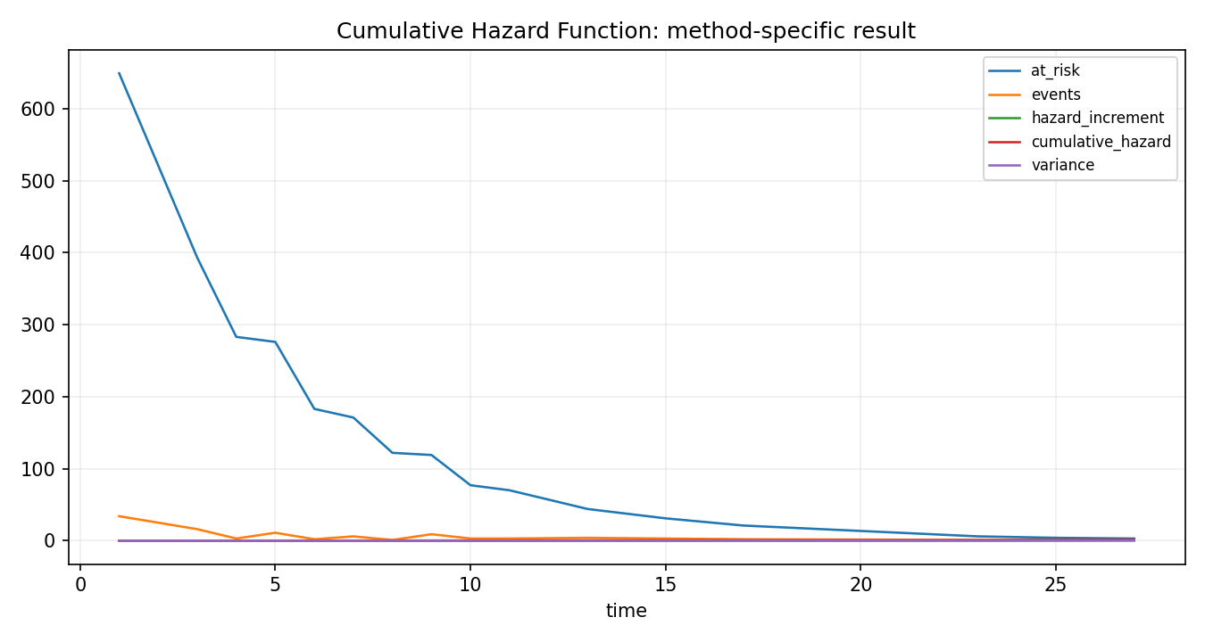
The Nelson–Aalen cumulative hazard was 0.312 at time 10 and 1.055 at time 25; the corresponding −ln KM values were 0.320 and 1.131.
What does Cumulative Hazard Function measure?
the total hazard accumulated from the time origin through a specified time
Cumulative Hazard Function focuses on the total hazard accumulated from the time origin through a specified time. The estimand must remain separate from related quantities such as ordinary probability, crude event proportion, mean duration, or an unrelated regression coefficient.
Method target
Cumulative Hazard Function is selected to translate event intensity over time into an additive cumulative scale connected to the survival function. The method is applied to ordered follow-up times and event indicators, not to a standalone numeric outcome with censoring ignored. The analysis therefore starts from risk sets and event times.
The worked example defines time as absences plus one and the primary event as G3 below 10. For Cumulative Hazard Function, these variables are used only to demonstrate the total hazard accumulated from the time origin through a specified time; they are not presented as naturally observed medical survival times.
What it does not establish
The procedure cannot create causality or a real-world failure process from cross-sectional student records. Its defensible output is the method-specific estimate or test under the stated coding, and cumulative hazard is additive and unbounded, unlike survival probability, which remains between zero and one.
Cumulative hazard is additive and unbounded, unlike survival probability, which remains between zero and one.
When should Cumulative Hazard Function be used?
Decision logic before software
Time outcome?
Confirm a meaningful duration from a common origin.
Event defined?
State event=1 and censor=0 unambiguously.
Method target?
Match Cumulative Hazard Function to the estimand.
Assumptions?
Audit censoring, risk sets, ties, and model form.
Reportable?
Retain numerical evidence and limitations.
Appropriate use
Choose this method when the research question is genuinely about the total hazard accumulated from the time origin through a specified time and the required assumptions can be defended. It is preferable to a simple mean or binary comparison because it retains event timing and censoring information relevant to adds event-to-risk-set increments so accumulated event intensity increases monotonically from zero.
Cumulative Hazard Function is especially useful when its specific estimand is more informative than an ordinary mean comparison or binary event analysis that discards follow-up time.
Inappropriate use
The exclusion rule for Cumulative Hazard Function is as important as the inclusion rule. It is unsuitable when the data lack a defensible time origin and status indicator, or when a descriptive estimator is being used as though it were an adjusted causal model. The matched files and examples are retained only because they use the same endpoint and specification. The Nelson–Aalen cumulative hazard is 0.1436 at time 5, 0.3124 at time 10, and 1.0548 at time 25.
Do not publish Cumulative Hazard Function output when the matching charts, PDFs, workbook, and dataset describe different definitions or model specifications.
Cumulative Hazard Function dataset and variable construction
The exact 649-row teaching structure
The bundled 649-row dataset is used specifically for direct accumulation of d_i/n_i increments and comparison with −ln Kaplan–Meier. All 100 event times contribute Nelson–Aalen increments, while 549 censored records remain in risk sets until their prepared duration and affect later denominators. The prepared endpoint remains a transparent teaching construction rather than natural clinical, mortality, or equipment-failure follow-up.
| Variable | Role | Coding | Audit note |
|---|---|---|---|
| surv_time | Duration | absences + 1 | Positive values from 1 to 33 |
| surv_event | Primary event | 1 when G3 < 10; 0 otherwise | 100 events and 549 censorings |
| school | Group | GP reference; MS comparison | 423 GP and 226 MS records |
| competing cause | Secondary event | failures > 0 among records without the primary event | 51 competing events |
| predictors | Cox covariates | age, parental education, travel/study time, failures, family relationship, free time, school, gender | Ten-term model |
Cumulative Hazard Function assumptions
Conditions required for a defensible result
A Valid Time-To-Event Construction
Cumulative Hazard Function requires a valid time-to-event construction. This condition is evaluated against the prepared duration, event coding, group structure, risk sets, and the method-specific result rather than assumed from the word nonparametric or from successful software execution.
Non-Informative Censoring
Cumulative Hazard Function requires non-informative censoring. This condition is evaluated against the prepared duration, event coding, group structure, risk sets, and the method-specific result rather than assumed from the word nonparametric or from successful software execution.
Correct Risk Sets
Cumulative Hazard Function requires correct risk sets. This condition is evaluated against the prepared duration, event coding, group structure, risk sets, and the method-specific result rather than assumed from the word nonparametric or from successful software execution.
Consistent Handling Of Ties
Cumulative Hazard Function requires consistent handling of ties. This condition is evaluated against the prepared duration, event coding, group structure, risk sets, and the method-specific result rather than assumed from the word nonparametric or from successful software execution.
Sufficient Tail Support
Cumulative Hazard Function requires sufficient tail support. This condition is evaluated against the prepared duration, event coding, group structure, risk sets, and the method-specific result rather than assumed from the word nonparametric or from successful software execution.
Clear Distinction Among Survival, Hazard, And Cumulative Hazard
For Cumulative Hazard Function, assumptions are assessed one by one using counts, curves, residuals, risk sets, or likelihood diagnostics appropriate to the procedure. The corresponding negative log Kaplan–Meier values are close but not identical because the estimators use different finite-sample constructions. Successful execution is not counted as evidence that the conditions hold.
Cumulative Hazard Function formula and mechanics
Native browser MathML and a plain-language audit trail
Cumulative Hazard Function uses this expression to estimate or test the total hazard accumulated from the time origin through a specified time. Every symbol should be linked to a risk set, event count, survival estimate, covariate, distribution parameter, or weight defined in the surrounding text.
Calculation sequence
- Sort positive durations and verify event/censor coding.
- Construct the exact risk set immediately before each event time.
- Calculate the Cumulative Hazard Function contribution defined by the formula.
- Accumulate products, sums, likelihood terms, or weighted contrasts as required.
- Attach uncertainty, diagnostics, and a conclusion that matches the estimand.
Formula interpretation
For Formula interpretation, the Cumulative Hazard Function review must connect every symbol to a risk set, event count, likelihood term, or model parameter. This method accumulates event-to-risk-set increments so total event intensity rises monotonically from zero; therefore the editor should compare Nelson–Aalen values with negative log Kaplan–Meier and inspect sparse late risk sets. The bundled example supplies the following numerical anchor: The Nelson–Aalen cumulative hazard was 0.312 at time 10 and 1.055 at time 25; the corresponding −ln KM values were 0.320 and 1.131.
The displayed expression uses browser-native MathML and ordinary semantic HTML. Its symbols correspond to the risk sets, event counts, weights, coefficients, or distribution parameters defined in this section; no remote rendering script or equation image is required.
Cumulative Hazard Function illustrative results
Values calculated from the included dataset
| Result item | Illustrative value |
|---|---|
| H(5) | 0.144 |
| H(10) | 0.312 |
| H(15) | 0.543 |
| H(20) | 0.638 |
| H(25) | 1.055 |
How to interpret Cumulative Hazard Function
From statistical output to a restrained conclusion
Primary conclusion
Hazard accumulates markedly in the tail
For Primary conclusion, the Cumulative Hazard Function review must translate the numerical result without overstating causality, equivalence, or natural follow-up. This method accumulates event-to-risk-set increments so total event intensity rises monotonically from zero; therefore the editor should compare Nelson–Aalen values with negative log Kaplan–Meier and inspect sparse late risk sets. The bundled example supplies the following numerical anchor: The Nelson–Aalen cumulative hazard was 0.312 at time 10 and 1.055 at time 25; the corresponding −ln KM values were 0.320 and 1.131.
Interpretation order
Cumulative Hazard Function in Python
Transparent data preparation and reproducible calculations
This Python section reconstructs the total hazard accumulated from the time origin through a specified time from explicit arrays and auditable intermediate tables. Adds event-to-risk-set increments so accumulated event intensity increases monotonically from zero, so the code below exposes the quantities that determine the final result.
import numpy as np

import pandas as pddf = pd.read_csv("dataset.csv")

time = pd.to_numeric(df["absences"]).to_numpy(float) + 1

event = (pd.to_numeric(df["G3"]) < 10).to_numpy(int)

S, H = 1.0, 0.0

rows=[]

for tj in np.sort(np.unique(time[event == 1])):

n = (time >= tj).sum()

d = ((time == tj) & (event == 1)).sum()

H += d/n

S *= 1-d/n

rows.append((tj,n,d,S,H,-np.log(S)))

print(pd.DataFrame(rows,columns=["time","risk","events","KM_S","NA_H","minus_log_KM"]))
Python verification checklist
The Python workflow for Cumulative Hazard Function begins by printing shapes, status counts, group coding, and intermediate quantities before the final statistic. Every event adds d_i/n_i to the cumulative scale, while censoring changes only later denominators. The saved script implements the fact that the method adds event-to-risk-set increments so accumulated event intensity increases monotonically from zero, which makes the calculation independently auditable.
Only topic-matching URLs from the uploaded register are embedded. When a Python, R, SPSS, or Excel file is absent, the article states that limitation rather than fabricating a filename or borrowing another post’s asset.
Cumulative Hazard Function in R
Independent survival-analysis validation
R provides an independent implementation of the same the total hazard accumulated from the time origin through a specified time. The script states status coding, factor references, and the function or manual calculation needed for this method instead of relying on defaults.
df <- read.csv("dataset.csv", stringsAsFactors=FALSE)

df$time <- as.numeric(df$absences) + 1

df$event <- ifelse(as.numeric(df$G3) < 10, 1, 0)

event_times <- sort(unique(df$time[df$event == 1]))

result <- data.frame(time=event_times, n_risk=NA_integer_, n_event=NA_integer_,

increment=NA_real_, cumulative_hazard=NA_real_)

H <- 0

for (i in seq_along(event_times)) {

tt <- event_times[i]

n <- sum(df$time >= tt)

d <- sum(df$time == tt & df$event == 1)

inc <- d/n; H <- H + inc

result[i,2:5] <- list(n, d, inc, H)

}

print(result)
R validation checklist
R provides an independent route for Cumulative Hazard Function with explicit formulas and saved output rather than a second decorative code block. The estimate is additive and may exceed one; it must not be described as a probability. The audit records package versions and uses the plan to compare the direct Nelson–Aalen path with negative log Kaplan–Meier values and inspect late jumps.
Cumulative Hazard Function in SPSS
Syntax-first setup and output audit
The SPSS workflow separates native procedures from extensions and preserves the event value in saved syntax. It is reviewed against the same dataset counts and interpretation used by the other software sections.
COMPUTE surv_time=absences+1.

COMPUTE surv_event=(G3<10).

KM surv_time /STATUS=surv_event(1) /PRINT TABLE /PLOT SURVIVAL HAZARD.

* Export the table and verify cumulative hazard against a manual Nelson–Aalen calculation.Cumulative Hazard Function in Excel
A visible calculation and reconciliation workbook
The Excel workbook exposes the arithmetic behind H(t) = ∫₀ᵗ h(u)du = −ln[S(t)] and reconciles selected rows with the programmatic output. It is an auditable calculation, not a black-box result.
Excel step 1
Build a unique event-time risk table.
Excel step 2
Update survival by multiplying 1-d/n.
Excel step 3
Update cumulative hazard by adding d/n.
Excel step 4
Calculate -LN(S) for comparison.
Excel step 5
Stop overinterpreting when the tail risk set becomes very small.
Excel controls
For Excel controls, the Cumulative Hazard Function review must make the spreadsheet an auditable calculation rather than a decorative download. This method accumulates event-to-risk-set increments so total event intensity rises monotonically from zero; therefore the editor should compare Nelson–Aalen values with negative log Kaplan–Meier and inspect sparse late risk sets. The bundled example supplies the following numerical anchor: The Nelson–Aalen cumulative hazard was 0.312 at time 10 and 1.055 at time 25; the corresponding −ln KM values were 0.320 and 1.131.
Cumulative Hazard Function charts and chart-specific interpretation
First chart full-width; remaining charts arranged in pairs
Media placement follows the verified workbook: the first chart spans the content width, later charts form responsive pairs, and every downloadable file remains tied to this post’s method and dataset definition.
Python chart 1 — Cumulative Hazard Function
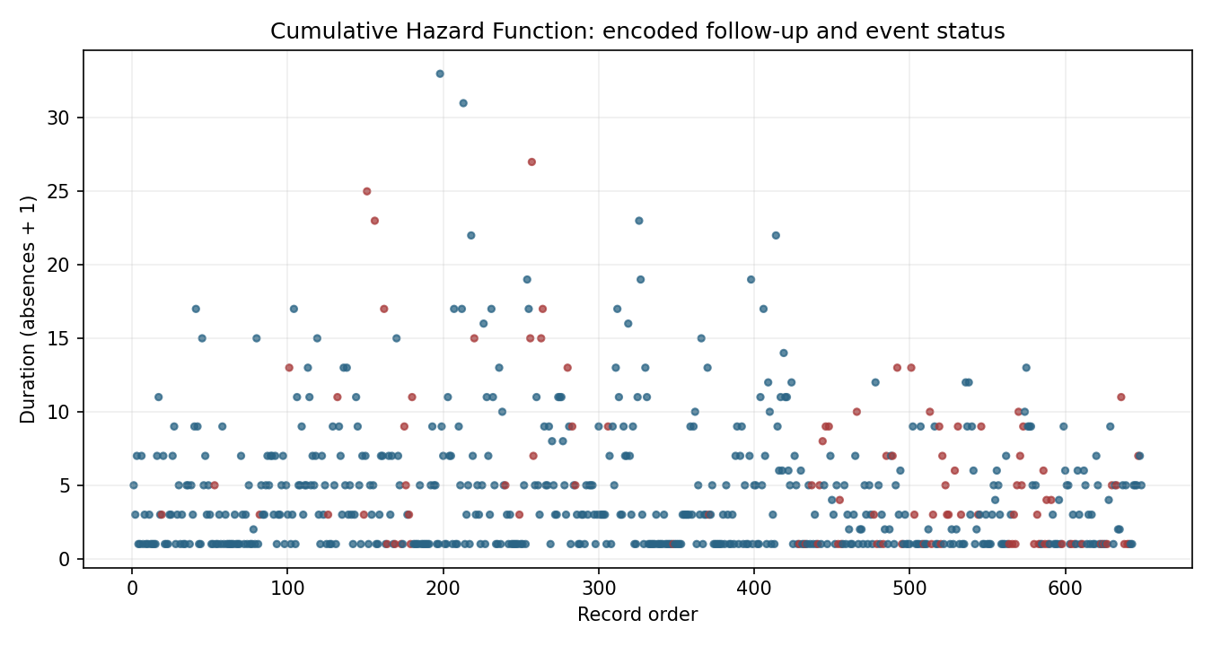
Python chart 1: shows the prepared 1–33 duration distribution, event/censor pattern, and where the survival estimator obtains most of its information. For this topic, the display should be read with the event definition and the fact that the method adds event-to-risk-set increments so accumulated event intensity increases monotonically from zero.
Python chart 2 — Cumulative Hazard Function
Python chart 2: summarizes the principal Cumulative Hazard Function output and the numerical components behind the reported conclusion. The Nelson–Aalen cumulative hazard was 0.312 at time 10 and 1.055 at time 25; the corresponding −ln KM values were 0.320 and 1.131.
Python chart 3 — Cumulative Hazard Function
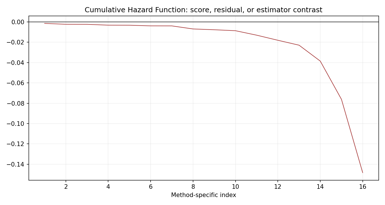
Python chart 3: examines the diagnostic path most relevant to the assumptions of this survival estimator. The review priority is to compare the direct Nelson–Aalen path with negative log Kaplan–Meier values and inspect late jumps; visible structure is a warning rather than decoration.
Python chart 4 — Cumulative Hazard Function
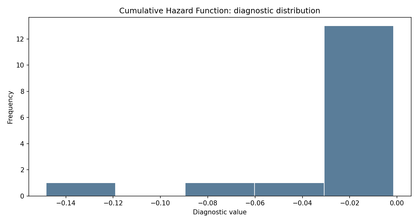
Python chart 4: places uncertainty, residuals, weighted contributions, or fitted discrepancies on a distributional scale. It supports the model or test audit but does not replace the natural-scale result or its confidence interval.
Python chart 5 — Cumulative Hazard Function
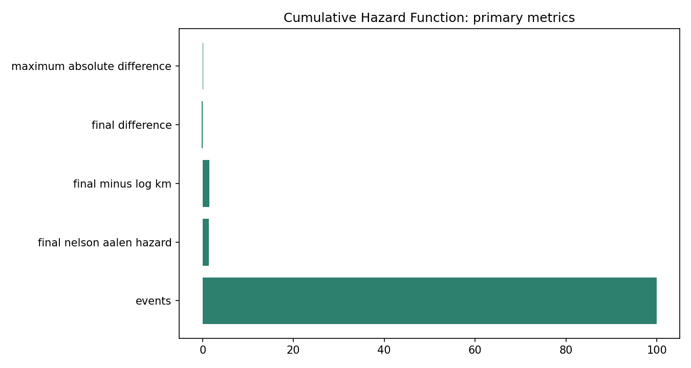
Python chart 5: collects the key verified metrics used in the article, including sample information and the method-specific estimate. Every displayed value must reconcile with dataset.csv and the downloadable Python output.
R chart 1 — Cumulative Hazard Function
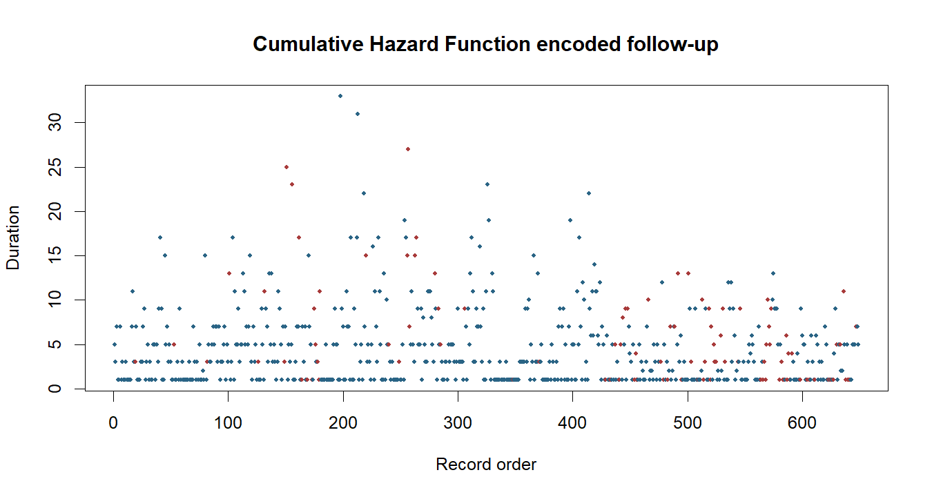
R chart 1 independently reproduces the prepared duration, event, and censoring structure for Cumulative Hazard Function. Read it with the declared event definition before comparing groups or fitted quantities.
R chart 2 — Cumulative Hazard Function
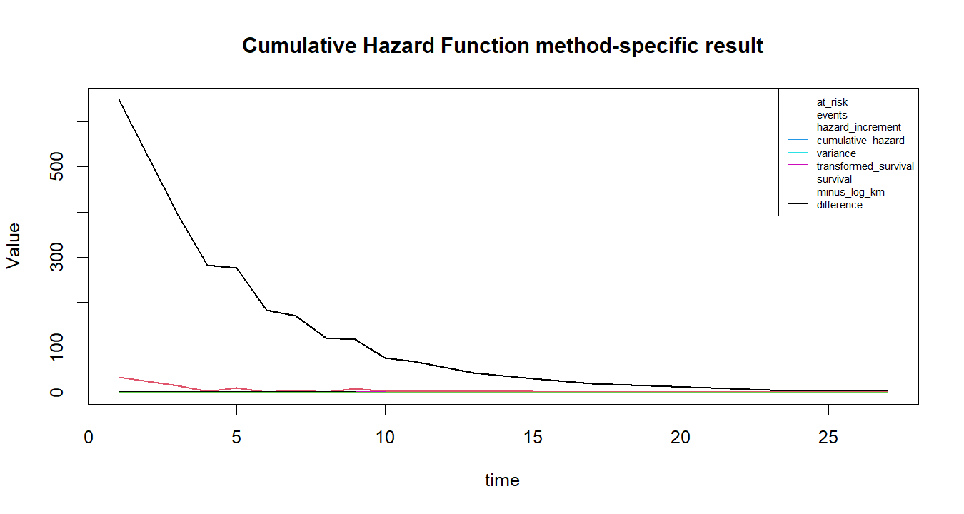
R chart 2 presents the benchmark output using R conventions. Its values should agree with the Python calculation after reference levels, tie handling, weighting, and status coding are aligned.
R chart 3 — Cumulative Hazard Function
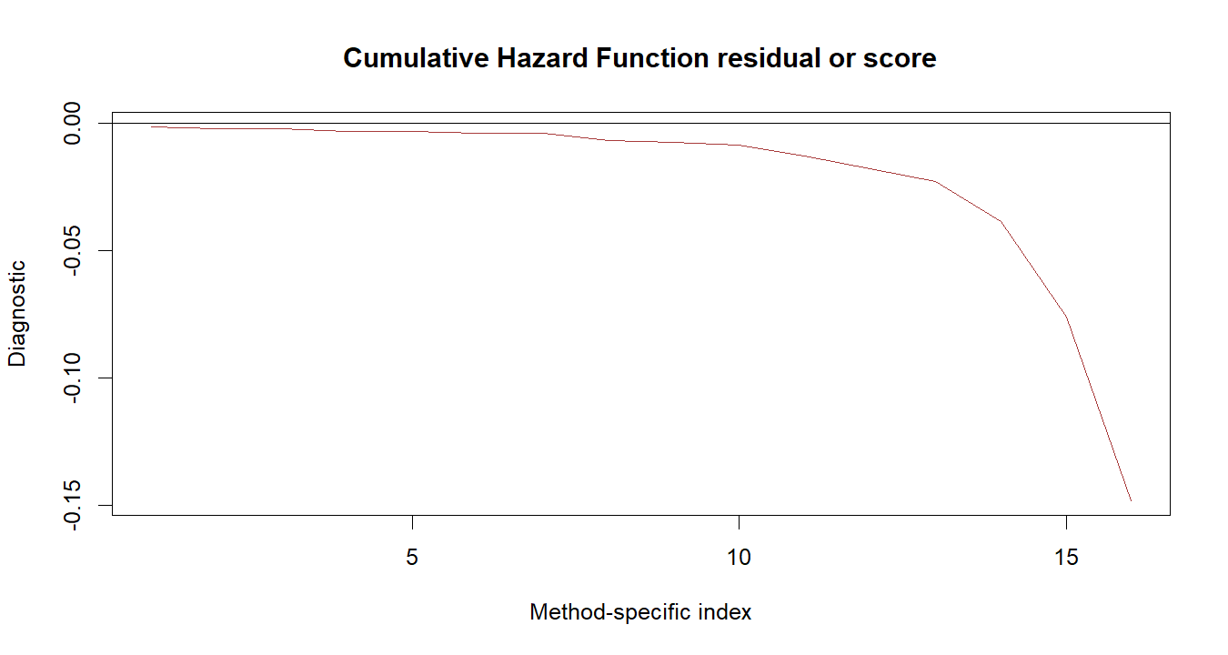
R chart 3 focuses on the diagnostic evidence for Cumulative Hazard Function. Visible departures or sparse-tail behavior should trigger a sensitivity analysis rather than a cosmetic interpretation.
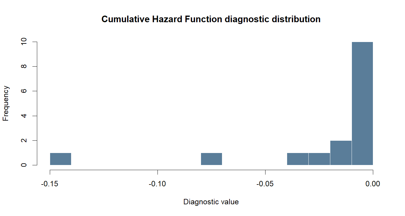
R chart 4 — Cumulative Hazard Function
R chart 4 displays uncertainty or residual structure on the scale used by the R workflow. It supports the numerical audit but does not replace the natural-scale estimate and its limitation.
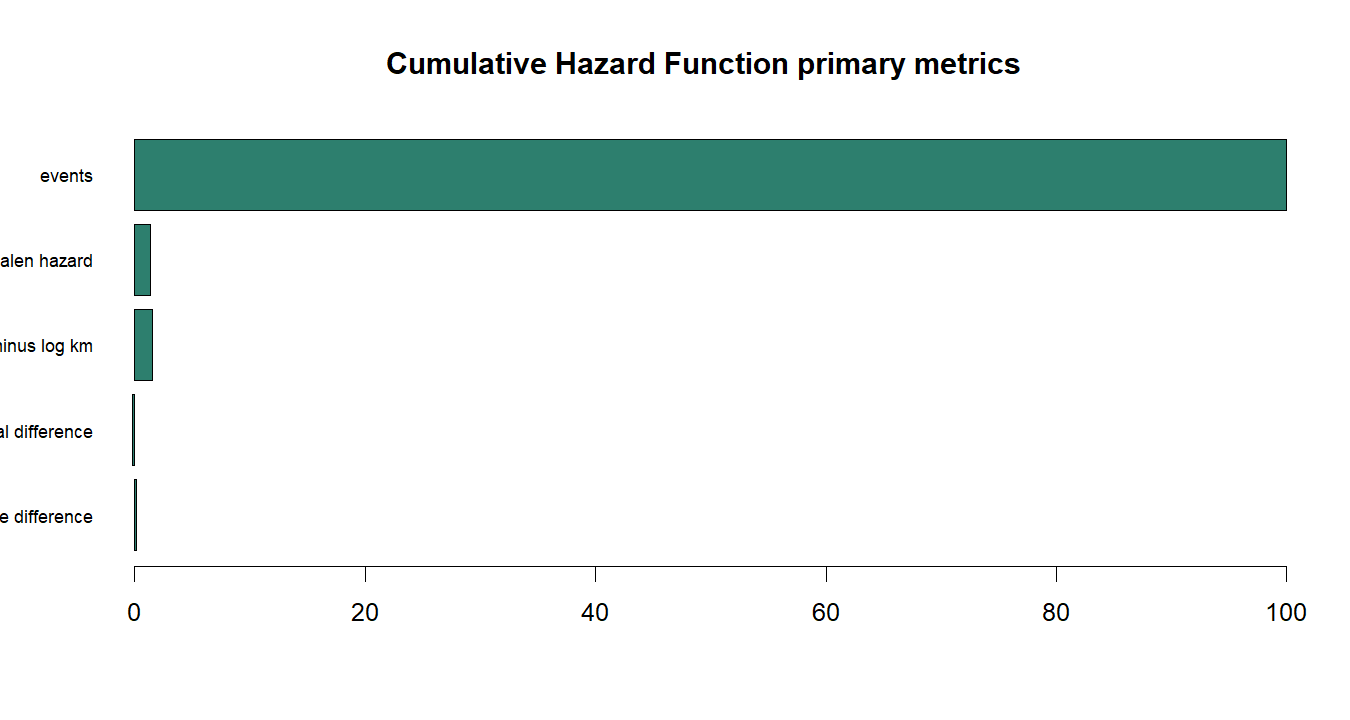
R chart 5 — Cumulative Hazard Function
R chart 5 consolidates the principal metrics used in the R output. Every annotation must reconcile with dataset.csv, the printed result, and the matched downloadable file.
Cumulative Hazard Function diagnostics and sensitivity analysis
Evidence required beyond the primary number
Data diagnostics
Before interpreting the primary result, verify the 649-row count, 100 events, 549 censorings, 1–33 duration range, GP/MS composition, tied times, and missing values. The method-specific review then asks analysts to compare the direct Nelson–Aalen path with negative log Kaplan–Meier values and inspect late jumps.
Method diagnostics
Diagnostics for Cumulative Hazard Function target the failure modes of this procedure rather than offering a generic residual checklist. Late jumps are based on small risk sets and therefore require visible tail qualifications. The specified review is to compare the direct Nelson–Aalen path with negative log Kaplan–Meier values and inspect late jumps; any unresolved problem limits the conclusion before publication.
Sensitivity diagnostics
Compare Cumulative Hazard Function with Kaplan–Meier survival, Nelson–Aalen cumulative hazard, life-table grouped estimates, parametric survival functions. Explain whether the substantive conclusion changes and why.
Full Cumulative Hazard Function publication audit
Method-specific checkpoints for content, data, formulas, results, and assets
1. Research estimand
Research estimand receives an explicit pass, warning, or fail assessment. State the exact population quantity and contrast before examining results. This is necessary because the method adds event-to-risk-set increments so accumulated event intensity increases monotonically from zero, and a different construction would answer a different survival question.
The Nelson–Aalen cumulative hazard is 0.1436 at time 5, 0.3124 at time 10, and 1.0548 at time 25. The result is meaningful only within the constructed endpoint and observed follow-up. The audit should compare the direct Nelson–Aalen path with negative log Kaplan–Meier values and inspect late jumps, then frame direction according to the principle that larger cumulative hazard means more accumulated event intensity, but the scale is not a probability.
2. Time origin
Time origin receives an explicit pass, warning, or fail assessment. Document what time zero represents and reject records measured from a different baseline. This is necessary because the method adds event-to-risk-set increments so accumulated event intensity increases monotonically from zero, and a different construction would answer a different survival question.
The corresponding negative log Kaplan–Meier values are close but not identical because the estimators use different finite-sample constructions. The article should retain this value in a saved table and connect it to its matching chart. Reviewers should also compare the direct Nelson–Aalen path with negative log Kaplan–Meier values and inspect late jumps, because larger cumulative hazard means more accumulated event intensity, but the scale is not a probability.
3. Event and status coding
The reviewer should pause at event and status coding and reproduce the relevant step. Describe every status value in words and verify its frequency before fitting. In this analysis the procedure adds event-to-risk-set increments so accumulated event intensity increases monotonically from zero; that mechanism sets the boundary for correct interpretation.
Every event adds d_i/n_i to the cumulative scale, while censoring changes only later denominators. Any discrepancy across Python, R, SPSS, or Excel must be traced to definitions or defaults. In addition, compare the direct Nelson–Aalen path with negative log Kaplan–Meier values and inspect late jumps; the reader should be told that larger cumulative hazard means more accumulated event intensity, but the scale is not a probability.
4. Censoring definition
This checkpoint asks whether censoring definition has been translated into executable analysis. Explain why a censored observation contributes to earlier risk sets and not later events. The method adds event-to-risk-set increments so accumulated event intensity increases monotonically from zero; therefore a generic survival-analysis explanation is not enough for this post.
The estimate is additive and may exceed one; it must not be described as a probability. This number is retained because it distinguishes the current method from neighboring procedures. The quality-control step is to compare the direct Nelson–Aalen path with negative log Kaplan–Meier values and inspect late jumps; the directional explanation follows the fact that larger cumulative hazard means more accumulated event intensity, but the scale is not a probability.
5. Duration scale
Duration scale defines the checkpoint for this article. Audit the numerical time scale and any recoding used to obtain it. Because the procedure adds event-to-risk-set increments so accumulated event intensity increases monotonically from zero, the reviewer must connect the source rows to that mechanism rather than infer correctness from the software label.
Late jumps are based on small risk sets and therefore require visible tail qualifications. The post links this evidence to the formula and saved output rather than repeating generic advice. A defensible review will compare the direct Nelson–Aalen path with negative log Kaplan–Meier values and inspect late jumps, and it will state clearly that larger cumulative hazard means more accumulated event intensity, but the scale is not a probability.
6. Risk-set or likelihood construction
Treat risk-set or likelihood construction as an analytical decision. Trace the core estimating equation to observable rows and event times. Here the method adds event-to-risk-set increments so accumulated event intensity increases monotonically from zero; a reproducible audit therefore records the relevant inputs, intermediate quantities, and settings before accepting the displayed result.
The cumulative-hazard curve is useful for model diagnostics and transformations, but it does not by itself test group differences. Any discrepancy across Python, R, SPSS, or Excel must be traced to definitions or defaults. In addition, compare the direct Nelson–Aalen path with negative log Kaplan–Meier values and inspect late jumps; the reader should be told that larger cumulative hazard means more accumulated event intensity, but the scale is not a probability.
7. Ties and discretization
Ties and discretization receives an explicit pass, warning, or fail assessment. Declare how simultaneous event times are aggregated or approximated. This is necessary because the method adds event-to-risk-set increments so accumulated event intensity increases monotonically from zero, and a different construction would answer a different survival question.
The Nelson–Aalen cumulative hazard is 0.1436 at time 5, 0.3124 at time 10, and 1.0548 at time 25. Any discrepancy across Python, R, SPSS, or Excel must be traced to definitions or defaults. In addition, compare the direct Nelson–Aalen path with negative log Kaplan–Meier values and inspect late jumps; the reader should be told that larger cumulative hazard means more accumulated event intensity, but the scale is not a probability.
8. Reference coding
Reference coding can invalidate an otherwise polished article. Establish reference coding before assigning better or worse direction. The reason is specific to this procedure: it adds event-to-risk-set increments so accumulated event intensity increases monotonically from zero. The final wording should state any unresolved limitation rather than hide it behind a p-value.
The corresponding negative log Kaplan–Meier values are close but not identical because the estimators use different finite-sample constructions. This is the concrete evidence used for the checkpoint. The sensitivity plan is to compare the direct Nelson–Aalen path with negative log Kaplan–Meier values and inspect late jumps; the narrative must not forget that larger cumulative hazard means more accumulated event intensity, but the scale is not a probability.
9. Missing-data handling
A strong account of missing-data handling names the decision and shows its consequence. Reconcile every omitted row and confirm that exclusions do not change status coding. Since the method adds event-to-risk-set increments so accumulated event intensity increases monotonically from zero, hidden defaults at this point would propagate into every later value.
Every event adds d_i/n_i to the cumulative scale, while censoring changes only later denominators. The numerical record supports a method-specific audit, but it does not remove design limitations. To test robustness, compare the direct Nelson–Aalen path with negative log Kaplan–Meier values and inspect late jumps; when stating direction, note that larger cumulative hazard means more accumulated event intensity, but the scale is not a probability.
10. Dependence and clustering
Treat dependence and clustering as an analytical decision. Assess whether repeated, matched, or nested records require robust or multilevel treatment. Here the method adds event-to-risk-set increments so accumulated event intensity increases monotonically from zero; a reproducible audit therefore records the relevant inputs, intermediate quantities, and settings before accepting the displayed result.
The estimate is additive and may exceed one; it must not be described as a probability. This evidence is read alongside the checkpoint rather than used as a substitute for it. The recommended diagnostic is to compare the direct Nelson–Aalen path with negative log Kaplan–Meier values and inspect late jumps, and the final interpretation should remember that larger cumulative hazard means more accumulated event intensity, but the scale is not a probability.
11. Information and event adequacy
Use information and event adequacy to challenge the draft rather than merely document it. Print the status mapping and reconcile each event total with the CSV. The relevant technical fact is that the estimator adds event-to-risk-set increments so accumulated event intensity increases monotonically from zero, which determines what must be checked in the stored output.
Late jumps are based on small risk sets and therefore require visible tail qualifications. The numerical record supports a method-specific audit, but it does not remove design limitations. To test robustness, compare the direct Nelson–Aalen path with negative log Kaplan–Meier values and inspect late jumps; when stating direction, note that larger cumulative hazard means more accumulated event intensity, but the scale is not a probability.
12. Tail support
Tail support can invalidate an otherwise polished article. Separate stable follow-up from the thin tail before generalizing results. The reason is specific to this procedure: it adds event-to-risk-set increments so accumulated event intensity increases monotonically from zero. The final wording should state any unresolved limitation rather than hide it behind a p-value.
The cumulative-hazard curve is useful for model diagnostics and transformations, but it does not by itself test group differences. Reproducing that figure from the bundled CSV is required before publication. The diagnostic sequence should compare the direct Nelson–Aalen path with negative log Kaplan–Meier values and inspect late jumps, while the substantive statement recognizes that larger cumulative hazard means more accumulated event intensity, but the scale is not a probability.
13. Uncertainty interval
Use uncertainty interval to challenge the draft rather than merely document it. Report sampling uncertainty on the natural scale and reproduce its calculation. The relevant technical fact is that the estimator adds event-to-risk-set increments so accumulated event intensity increases monotonically from zero, which determines what must be checked in the stored output.
For 13. Uncertainty interval, the Cumulative Hazard Function review must record a method-specific publication checkpoint and the evidence required to pass it. This method accumulates event-to-risk-set increments so total event intensity rises monotonically from zero; therefore the editor should compare Nelson–Aalen values with negative log Kaplan–Meier and inspect sparse late risk sets. The bundled example supplies the following numerical anchor: The Nelson–Aalen cumulative hazard was 0.312 at time 10 and 1.055 at time 25; the corresponding −ln KM values were 0.320 and 1.131.
14. Null hypothesis and p-value
At null hypothesis and p-value, the article must move from terminology to evidence. Explain what the p-value conditions on and what it cannot establish. Its defining computation adds event-to-risk-set increments so accumulated event intensity increases monotonically from zero, and the audit should show where the required quantities appear in the CSV or derived table.
The corresponding negative log Kaplan–Meier values are close but not identical because the estimators use different finite-sample constructions. That checkpoint is considered complete only when the same value appears in code, table, and interpretation. The robustness review should compare the direct Nelson–Aalen path with negative log Kaplan–Meier values and inspect late jumps; the direction statement remains governed by the fact that larger cumulative hazard means more accumulated event intensity, but the scale is not a probability.
15. Effect magnitude
The publication test at effect magnitude is practical: could another analyst rebuild the same result from dataset.csv? Translate the numerical output into the method’s own effect scale. That standard matters because this approach adds event-to-risk-set increments so accumulated event intensity increases monotonically from zero.
Every event adds d_i/n_i to the cumulative scale, while censoring changes only later denominators. The result is meaningful only within the constructed endpoint and observed follow-up. The audit should compare the direct Nelson–Aalen path with negative log Kaplan–Meier values and inspect late jumps, then frame direction according to the principle that larger cumulative hazard means more accumulated event intensity, but the scale is not a probability.
16. Software defaults
Treat software defaults as an analytical decision. Record package versions, defaults, factor coding, convergence, and tie settings. Here the method adds event-to-risk-set increments so accumulated event intensity increases monotonically from zero; a reproducible audit therefore records the relevant inputs, intermediate quantities, and settings before accepting the displayed result.
The estimate is additive and may exceed one; it must not be described as a probability. That result becomes publishable only after its risk-set, likelihood, or coding trail is reconciled. A useful next check is to compare the direct Nelson–Aalen path with negative log Kaplan–Meier values and inspect late jumps. Directional language must remain consistent with the rule that larger cumulative hazard means more accumulated event intensity, but the scale is not a probability.
17. Cross-software reconciliation
The reviewer should pause at cross-software reconciliation and reproduce the relevant step. Reconcile output differences by checking definitions before blaming numerical software. In this analysis the procedure adds event-to-risk-set increments so accumulated event intensity increases monotonically from zero; that mechanism sets the boundary for correct interpretation.
Late jumps are based on small risk sets and therefore require visible tail qualifications. The article should retain this value in a saved table and connect it to its matching chart. Reviewers should also compare the direct Nelson–Aalen path with negative log Kaplan–Meier values and inspect late jumps, because larger cumulative hazard means more accumulated event intensity, but the scale is not a probability.
18. Chart-to-table audit
The reviewer should pause at chart-to-table audit and reproduce the relevant step. Reject any image or download whose filename, values, or method label belongs to another post. In this analysis the procedure adds event-to-risk-set increments so accumulated event intensity increases monotonically from zero; that mechanism sets the boundary for correct interpretation.
The cumulative-hazard curve is useful for model diagnostics and transformations, but it does not by itself test group differences. The article should retain this value in a saved table and connect it to its matching chart. Reviewers should also compare the direct Nelson–Aalen path with negative log Kaplan–Meier values and inspect late jumps, because larger cumulative hazard means more accumulated event intensity, but the scale is not a probability.
19. Sensitivity specification
The reviewer should pause at sensitivity specification and reproduce the relevant step. Repeat the analysis under a defensible neighboring specification and explain the comparison. In this analysis the procedure adds event-to-risk-set increments so accumulated event intensity increases monotonically from zero; that mechanism sets the boundary for correct interpretation.
The Nelson–Aalen cumulative hazard is 0.1436 at time 5, 0.3124 at time 10, and 1.0548 at time 25. The article should retain this value in a saved table and connect it to its matching chart. Reviewers should also compare the direct Nelson–Aalen path with negative log Kaplan–Meier values and inspect late jumps, because larger cumulative hazard means more accumulated event intensity, but the scale is not a probability.
20. Scientific limitation
This checkpoint asks whether scientific limitation has been translated into executable analysis. Keep inference inside the observed design, coding, and follow-up window. The method adds event-to-risk-set increments so accumulated event intensity increases monotonically from zero; therefore a generic survival-analysis explanation is not enough for this post.
For 20. Scientific limitation, the Cumulative Hazard Function review must record a method-specific publication checkpoint and the evidence required to pass it. This method accumulates event-to-risk-set increments so total event intensity rises monotonically from zero; therefore the editor should compare Nelson–Aalen values with negative log Kaplan–Meier and inspect sparse late risk sets. The bundled example supplies the following numerical anchor: The Nelson–Aalen cumulative hazard was 0.312 at time 10 and 1.055 at time 25; the corresponding −ln KM values were 0.320 and 1.131.
21. Generalizability boundary
The reviewer should pause at generalizability boundary and reproduce the relevant step. Separate computational correctness from scientific validity and causal interpretation. In this analysis the procedure adds event-to-risk-set increments so accumulated event intensity increases monotonically from zero; that mechanism sets the boundary for correct interpretation.
Every event adds d_i/n_i to the cumulative scale, while censoring changes only later denominators. This evidence is read alongside the checkpoint rather than used as a substitute for it. The recommended diagnostic is to compare the direct Nelson–Aalen path with negative log Kaplan–Meier values and inspect late jumps, and the final interpretation should remember that larger cumulative hazard means more accumulated event intensity, but the scale is not a probability.
22. Reproducible record
Before interpreting the principal estimate, resolve reproducible record. Preserve the CSV, transformation rules, code, output, metadata, and matched URLs. The calculation adds event-to-risk-set increments so accumulated event intensity increases monotonically from zero, so any mismatch in timing, coding, or risk-set construction can change the target quantity even when the program completes normally.
The estimate is additive and may exceed one; it must not be described as a probability. That checkpoint is considered complete only when the same value appears in code, table, and interpretation. The robustness review should compare the direct Nelson–Aalen path with negative log Kaplan–Meier values and inspect late jumps; the direction statement remains governed by the fact that larger cumulative hazard means more accumulated event intensity, but the scale is not a probability.
23. Publication language
Publication language is reviewed separately from statistical significance. Make the published record independently reproducible and free of unsupported wording. For this survival estimator, the core operation adds event-to-risk-set increments so accumulated event intensity increases monotonically from zero; the prose, formula, table, and chart must all describe that same operation.
For 23. Publication language, the Cumulative Hazard Function review must record a method-specific publication checkpoint and the evidence required to pass it. This method accumulates event-to-risk-set increments so total event intensity rises monotonically from zero; therefore the editor should compare Nelson–Aalen values with negative log Kaplan–Meier and inspect sparse late risk sets. The bundled example supplies the following numerical anchor: The Nelson–Aalen cumulative hazard was 0.312 at time 10 and 1.055 at time 25; the corresponding −ln KM values were 0.320 and 1.131.
24. SEO and asset consistency
Before interpreting the principal estimate, resolve seo and asset consistency. Reject any image or download whose filename, values, or method label belongs to another post. The calculation adds event-to-risk-set increments so accumulated event intensity increases monotonically from zero, so any mismatch in timing, coding, or risk-set construction can change the target quantity even when the program completes normally.
The cumulative-hazard curve is useful for model diagnostics and transformations, but it does not by itself test group differences. This evidence is read alongside the checkpoint rather than used as a substitute for it. The recommended diagnostic is to compare the direct Nelson–Aalen path with negative log Kaplan–Meier values and inspect late jumps, and the final interpretation should remember that larger cumulative hazard means more accumulated event intensity, but the scale is not a probability.
25. Estimator identity
Before interpreting the principal estimate, resolve estimator identity. Define the decision operationally and show how it was checked. The calculation adds event-to-risk-set increments so accumulated event intensity increases monotonically from zero, so any mismatch in timing, coding, or risk-set construction can change the target quantity even when the program completes normally.
The Nelson–Aalen cumulative hazard is 0.1436 at time 5, 0.3124 at time 10, and 1.0548 at time 25. This evidence is read alongside the checkpoint rather than used as a substitute for it. The recommended diagnostic is to compare the direct Nelson–Aalen path with negative log Kaplan–Meier values and inspect late jumps, and the final interpretation should remember that larger cumulative hazard means more accumulated event intensity, but the scale is not a probability.
26. Variance construction
A strong account of variance construction names the decision and shows its consequence. Connect the standard error or interval to the estimator actually used. Since the method adds event-to-risk-set increments so accumulated event intensity increases monotonically from zero, hidden defaults at this point would propagate into every later value.
The corresponding negative log Kaplan–Meier values are close but not identical because the estimators use different finite-sample constructions. Any discrepancy across Python, R, SPSS, or Excel must be traced to definitions or defaults. In addition, compare the direct Nelson–Aalen path with negative log Kaplan–Meier values and inspect late jumps; the reader should be told that larger cumulative hazard means more accumulated event intensity, but the scale is not a probability.
27. Median and quantiles
This checkpoint asks whether median and quantiles has been translated into executable analysis. Document the evidence and the consequence of a warning or failure. The method adds event-to-risk-set increments so accumulated event intensity increases monotonically from zero; therefore a generic survival-analysis explanation is not enough for this post.
For 27. Median and quantiles, the Cumulative Hazard Function review must record a method-specific publication checkpoint and the evidence required to pass it. This method accumulates event-to-risk-set increments so total event intensity rises monotonically from zero; therefore the editor should compare Nelson–Aalen values with negative log Kaplan–Meier and inspect sparse late risk sets. The bundled example supplies the following numerical anchor: The Nelson–Aalen cumulative hazard was 0.312 at time 10 and 1.055 at time 25; the corresponding −ln KM values were 0.320 and 1.131.
28. Step placement and continuity
The publication test at step placement and continuity is practical: could another analyst rebuild the same result from dataset.csv? Define the decision operationally and show how it was checked. That standard matters because this approach adds event-to-risk-set increments so accumulated event intensity increases monotonically from zero.
The estimate is additive and may exceed one; it must not be described as a probability. This is the concrete evidence used for the checkpoint. The sensitivity plan is to compare the direct Nelson–Aalen path with negative log Kaplan–Meier values and inspect late jumps; the narrative must not forget that larger cumulative hazard means more accumulated event intensity, but the scale is not a probability.
29. Exact times versus intervals
The reviewer should pause at exact times versus intervals and reproduce the relevant step. Connect this checkpoint to a saved calculation rather than a generic claim. In this analysis the procedure adds event-to-risk-set increments so accumulated event intensity increases monotonically from zero; that mechanism sets the boundary for correct interpretation.
Late jumps are based on small risk sets and therefore require visible tail qualifications. This number is retained because it distinguishes the current method from neighboring procedures. The quality-control step is to compare the direct Nelson–Aalen path with negative log Kaplan–Meier values and inspect late jumps; the directional explanation follows the fact that larger cumulative hazard means more accumulated event intensity, but the scale is not a probability.
30. Censor marks and withdrawals
This checkpoint asks whether censor marks and withdrawals has been translated into executable analysis. Verify that censoring is represented as status information rather than discarded rows. The method adds event-to-risk-set increments so accumulated event intensity increases monotonically from zero; therefore a generic survival-analysis explanation is not enough for this post.
The cumulative-hazard curve is useful for model diagnostics and transformations, but it does not by itself test group differences. That checkpoint is considered complete only when the same value appears in code, table, and interpretation. The robustness review should compare the direct Nelson–Aalen path with negative log Kaplan–Meier values and inspect late jumps; the direction statement remains governed by the fact that larger cumulative hazard means more accumulated event intensity, but the scale is not a probability.
31. Monotonicity and bounds
At monotonicity and bounds, the article must move from terminology to evidence. Define the decision operationally and show how it was checked. Its defining computation adds event-to-risk-set increments so accumulated event intensity increases monotonically from zero, and the audit should show where the required quantities appear in the CSV or derived table.
The Nelson–Aalen cumulative hazard is 0.1436 at time 5, 0.3124 at time 10, and 1.0548 at time 25. This number is retained because it distinguishes the current method from neighboring procedures. The quality-control step is to compare the direct Nelson–Aalen path with negative log Kaplan–Meier values and inspect late jumps; the directional explanation follows the fact that larger cumulative hazard means more accumulated event intensity, but the scale is not a probability.
32. Tail transformation
A strong account of tail transformation names the decision and shows its consequence. Check whether sparse risk sets support the requested estimate or coefficient complexity. Since the method adds event-to-risk-set increments so accumulated event intensity increases monotonically from zero, hidden defaults at this point would propagate into every later value.
The corresponding negative log Kaplan–Meier values are close but not identical because the estimators use different finite-sample constructions. Reproducing that figure from the bundled CSV is required before publication. The diagnostic sequence should compare the direct Nelson–Aalen path with negative log Kaplan–Meier values and inspect late jumps, while the substantive statement recognizes that larger cumulative hazard means more accumulated event intensity, but the scale is not a probability.
33. Estimation versus hypothesis testing
Estimation versus hypothesis testing receives an explicit pass, warning, or fail assessment. Document the evidence and the consequence of a warning or failure. This is necessary because the method adds event-to-risk-set increments so accumulated event intensity increases monotonically from zero, and a different construction would answer a different survival question.
For 33. Estimation versus hypothesis testing, the Cumulative Hazard Function review must record a method-specific publication checkpoint and the evidence required to pass it. This method accumulates event-to-risk-set increments so total event intensity rises monotonically from zero; therefore the editor should compare Nelson–Aalen values with negative log Kaplan–Meier and inspect sparse late risk sets. The bundled example supplies the following numerical anchor: The Nelson–Aalen cumulative hazard was 0.312 at time 10 and 1.055 at time 25; the corresponding −ln KM values were 0.320 and 1.131.
34. Practical time horizons
Use practical time horizons to challenge the draft rather than merely document it. Define the decision operationally and show how it was checked. The relevant technical fact is that the estimator adds event-to-risk-set increments so accumulated event intensity increases monotonically from zero, which determines what must be checked in the stored output.
The estimate is additive and may exceed one; it must not be described as a probability. The article should retain this value in a saved table and connect it to its matching chart. Reviewers should also compare the direct Nelson–Aalen path with negative log Kaplan–Meier values and inspect late jumps, because larger cumulative hazard means more accumulated event intensity, but the scale is not a probability.
Final Cumulative Hazard Function release decision
This draft is released only when its exact formula, event definition, software settings, numerical result, chart captions, download files, and contextual links agree. The central computational mechanism is that it adds event-to-risk-set increments so accumulated event intensity increases monotonically from zero. That statement differentiates the article from the other twenty survival posts and prevents a shared template from substituting for method-specific explanation.
The final robustness record directs the editor to compare the direct Nelson–Aalen path with negative log Kaplan–Meier values and inspect late jumps. The directional interpretation remains: larger cumulative hazard means more accumulated event intensity, but the scale is not a probability. Because the example is built from absences and G3 in a student-performance dataset, publication must keep the teaching-purpose limitation visible and must not recast the endpoint as clinical survival, mortality, equipment failure, or causal evidence.
Cumulative Hazard Function compared with related methods
Choose the method by estimand, not menu proximity
| Related method | Comparison question |
|---|---|
| Kaplan–Meier survival | Kaplan–meier survival estimates event-free probability through conditional product-limit factors. Compare it with the present method by checking the estimand, censor handling, weight or distribution, uncertainty, and practical interpretation; retain Cumulative Hazard Function only when the total hazard accumulated from the time origin through a specified time is the actual target. |
| Nelson–Aalen cumulative hazard | Nelson–aalen cumulative hazard targets accumulated hazard instead of survival probability. Compare it with the present method by checking the estimand, censor handling, weight or distribution, uncertainty, and practical interpretation; retain Cumulative Hazard Function only when the total hazard accumulated from the time origin through a specified time is the actual target. |
| life-table grouped estimates | Life-table grouped estimates summarize interval failure and survival with a withdrawal convention. Compare it with the present method by checking the estimand, censor handling, weight or distribution, uncertainty, and practical interpretation; retain Cumulative Hazard Function only when the total hazard accumulated from the time origin through a specified time is the actual target. |
| parametric survival functions | Parametric survival functions use a specified distribution to smooth and potentially extrapolate the curve. Compare it with the present method by checking the estimand, censor handling, weight or distribution, uncertainty, and practical interpretation; retain Cumulative Hazard Function only when the total hazard accumulated from the time origin through a specified time is the actual target. |
How to report Cumulative Hazard Function
A complete, restrained result statement
Reporting template
“A Cumulative Hazard Function analysis used 649 records from dataset(100).csv. Duration was defined as absences plus one, and the event indicator equaled one when G3 was below 10; 100 events and 549 right-censored observations were available. The Nelson–Aalen cumulative hazard was 0.312 at time 10 and 1.055 at time 25; the corresponding −ln KM values were 0.320 and 1.131. The analysis documented event coding, reference groups, risk sets, ties, assumptions, software settings, diagnostics, matching files, and the educational nature of the prepared survival endpoint.”
Include
Avoid calling hazard a probability, treating censoring as missingness, or converting a nonsignificant result into proof of equality. The final sentence should answer the stated estimand and no broader question.
Avoid
A complete report states the prepared time origin, event and censor codes, sample and event counts, group or predictor reference, exact method, formula, estimate or statistic, uncertainty, and the relevant diagnostics. It then gives this result: The Nelson–Aalen cumulative hazard was 0.312 at time 10 and 1.055 at time 25; the corresponding −ln KM values were 0.320 and 1.131.
Cumulative Hazard Function downloads
Only assets assigned to this topic after filename and extension audit
The download panel contains only URLs whose filenames and extensions match this topic in the source register. The plugin does not infer a missing asset from another post or alter the registered media path.
Cumulative Hazard Function frequently asked questions
Method-specific answers for draft review
What does Cumulative Hazard Function measure?
Cumulative Hazard Function is used for the estimand defined in this article. It accumulates event-to-risk-set increments so total event intensity rises monotonically from zero. The interpretation remains conditional on the stated time origin, event code, censoring rule, group or predictor coding, and any distributional or proportionality assumptions.
When should Cumulative Hazard Function be used?
Use Cumulative Hazard Function when the research objective requires direct accumulation of d_i/n_i increments and comparison with −ln Kaplan–Meier and the assumptions listed in the article are defensible. The method is inappropriate when a different event type, time emphasis, adjustment strategy, or hazard shape is the scientific target.
What data are used in this Cumulative Hazard Function example?
All 100 event times contribute Nelson–Aalen increments, while 549 censored records remain in risk sets until their prepared duration and affect later denominators. All values come from the uploaded 649-row file and the disclosed absences-plus-one/G3 event construction.
What is the main Cumulative Hazard Function result?
The result is summarized by this verified anchor: The Nelson–Aalen cumulative hazard was 0.312 at time 10 and 1.055 at time 25; the corresponding −ln KM values were 0.320 and 1.131. It should be read together with the method-specific assumptions, uncertainty, and the teaching-endpoint limitation rather than as a stand-alone causal conclusion.
How does censoring affect Cumulative Hazard Function?
Censored records contribute to risk sets or likelihood survival terms until their observed duration. Their handling matters because accumulates event-to-risk-set increments so total event intensity rises monotonically from zero; treating censoring as an event or deleting censored rows would change the estimate and usually bias the analysis.
How are ties handled in Cumulative Hazard Function?
The prepared durations are integer-valued, so tied times are common. The article states the exact pooled-event rule, weight, or Efron/Breslow approximation used for Cumulative Hazard Function, and software results should be reconciled only after those defaults match.
Can Cumulative Hazard Function be completed in Python?
Yes. The Python section reconstructs the data fields and exposes the intermediate quantities required for Cumulative Hazard Function. It prints the benchmark result and supports the diagnostic task to compare Nelson–Aalen values with negative log Kaplan–Meier and inspect sparse late risk sets.
Can Cumulative Hazard Function be completed in R?
Yes. The R section uses a method-appropriate survival or competing-risk routine, declares factor references and tie or weighting settings, and provides an independent check of the benchmark result for Cumulative Hazard Function.
Can Cumulative Hazard Function be completed in SPSS?
SPSS is used only where a native procedure matches Cumulative Hazard Function. When no exact native command exists, the post describes SPSS as a data-management, charting, or integration route and does not rename a different test or model.
How does Excel support Cumulative Hazard Function?
Excel supports Cumulative Hazard Function by displaying d_i/n_i increments, their cumulative sum, and comparison with −ln[S(t)] in visible cells. The matching workbook must reproduce selected Python and R benchmark values and retain the exact event, censoring, group, tie, and interval definitions.
What is the largest reporting mistake for Cumulative Hazard Function?
The largest Cumulative Hazard Function reporting error is calling cumulative hazard a probability or expecting it to stay below one. The article also keeps the teaching-endpoint limitation visible so the worked result is not presented as causal or naturally observed survival evidence.
Which internal guides support Cumulative Hazard Function?
Start with Nelson Aalen Estimator because it provides the nearest check on direct accumulation of d_i/n_i increments and comparison with −ln Kaplan–Meier. Use Survival Function, Kaplan Meier Survival Curve, Hazard Ratio to compare weighting, probability scale, model assumptions, or software implementation; each link has a specific methodological role rather than serving as generic navigation.