
Hypothesis Testing, Mean Comparison, Confidence Intervals and Effect Size
Independent Samples T Test: Formula, Interpretation, SPSS, Python, R and Excel Guide
Independent Samples T Test is used to compare the means of two unrelated groups on one continuous outcome. In this real-data example, we compare final exam grade G3 between two school groups, GP and MS, from the student performance dataset. This guide explains the Independent Samples T Test with actual results, SPSS-style interpretation, Python charts, R validation charts, formulas, assumptions, confidence intervals, effect size, APA wording and Excel workflow.
Quick Answer: Independent Samples T Test Result
The Independent Samples T Test showed that students in GP scored significantly higher on G3 final grade than students in MS. The GP group had a mean of 12.577, while the MS group had a mean of 10.650. The mean difference was 1.926 points.
The test statistic was t(647) = 7.54, with p < .001. The 95% confidence interval for the mean difference was [1.425, 2.428], which does not include zero. That means the difference is statistically significant. The estimated effect size was approximately Cohen’s d = 0.62, which is usually interpreted as a medium practical effect.
Final interpretation: Reject the null hypothesis. There is strong evidence that the average G3 score differs between GP and MS, and the direction of the difference shows that GP students performed better on average.
Important note: Statistical significance tells us the difference is unlikely to be due to sampling error alone. Practical meaning comes from the effect size, the size of the mean gap, and the real educational context.
Table of Contents
- What Is an Independent Samples T Test?
- Independent Samples T Test Formula
- Null and Alternative Hypotheses
- Assumptions of the Independent Samples T Test
- Dataset and Variables Used
- Actual Results Summary
- SPSS-Style Interpretation
- Python Chart-by-Chart Interpretation
- R Chart-by-Chart Validation
- SPSS, R, Python and Excel Workflows
- Code Blocks
- APA Reporting
- Common Mistakes
- When to Use the Independent Samples T Test
- Downloads and Resources
- Related Guides
- FAQs
What Is an Independent Samples T Test?
An Independent Samples T Test compares the means of two unrelated groups on a continuous outcome. It answers a simple but important research question: is the average outcome in one group different from the average outcome in another group?
In this example, the two groups are school categories: GP and MS. The outcome variable is G3, the final exam grade. Because each student belongs to only one school group, the groups are independent. That makes the Independent Samples T Test the correct parametric method.
This test is sometimes called the independent t test, two sample t test, or unpaired t test. It is one of the most widely used procedures in quantitative research because it is easy to apply and easy to interpret.
Simple definition: The Independent Samples T Test checks whether two unrelated groups have the same population mean or whether their means differ by more than we would expect from random sampling variation.
Before using the test, it is good practice to understand related topics such as the null and alternative hypothesis, p value, confidence interval, standard deviation, and parametric vs nonparametric tests.
Independent Samples T Test Formula
The basic test compares the difference between two sample means relative to the standard error of that difference:
For the equal-variances version of the Independent Samples T Test, the pooled standard deviation is:
The standard error of the mean difference is then:
| Symbol | Meaning | Interpretation |
|---|---|---|
| X̄1, X̄2 | Group means | Average score in each group. |
| s1, s2 | Group standard deviations | Spread of scores within each group. |
| n1, n2 | Group sample sizes | Number of observations in each group. |
| SE | Standard error of the difference | Sampling variability in the mean difference. |
| t | t statistic | Observed mean difference expressed in SE units. |
Worked-data version: In this example, the observed mean difference is 1.926, the pooled standard deviation is about 3.100, the standard error is about 0.255, and the final test statistic is t = 7.54.
Null and Alternative Hypotheses for the Independent Samples T Test
The Independent Samples T Test evaluates whether the two population means are equal.
| Hypothesis | Statement | Meaning |
|---|---|---|
| Null hypothesis (H0) | μGP = μMS | The average G3 score is the same in both school groups. |
| Alternative hypothesis (H1) | μGP ≠ μMS | The average G3 score differs between GP and MS. |
This example uses a two-tailed test because the question is whether the groups differ, not whether one group must be larger in a pre-specified direction. If you want a directional version, see the one tailed t test guide.
Decision: Because p < .001, we reject H0. The data provide very strong evidence that the mean G3 score differs between GP and MS.
Assumptions of the Independent Samples T Test
Like other parametric tests, the Independent Samples T Test relies on a set of assumptions. Good reporting should always discuss them.
| Assumption | Status in This Example | Interpretation |
|---|---|---|
| Independent groups | Satisfied | Each student belongs to one school only, so the groups are unrelated. |
| Continuous dependent variable | Satisfied | G3 is a numeric final grade and is treated as continuous. |
| Approximate normality within groups | Reasonably acceptable | The histograms and boxplots show some skew and low-score outliers, but both samples are large, making the t test robust. |
| Homogeneity of variances | Should be checked | The MS group has a larger SD (3.834) than GP (2.626), so a formal Levene Test should be reported when available. |
The provided chart outputs do not display the numeric Levene statistic directly. However, the standard deviation comparison chart clearly shows that MS has more variability than GP. In a full SPSS table, report the Levene test p-value and choose the equal-variances or unequal-variances row accordingly.
Even so, the group difference is large enough that the practical conclusion is stable. A Welch-style robustness check using the actual group summaries still gives a highly significant result, so the decision would not change.
Practical interpretation: Assumptions are not there to block analysis. They help you decide how cautious to be and whether you need a robust alternative or extra reporting detail.
Dataset and Variables Used
This worked example uses the student performance dataset, where school is the grouping variable and G3 is the dependent variable. The two school groups are:
- GP = Gabriel Pereira
- MS = Mousinho da Silveira
The total number of valid observations in this analysis is 649. The group counts are:
| Group | n | Mean G3 | SD | Approx. 95% CI for Mean |
|---|---|---|---|---|
| GP | 423 | 12.577 | 2.626 | 12.326 to 12.828 |
| MS | 226 | 10.650 | 3.834 | 10.147 to 11.153 |
The outcome G3 is the final exam grade. Because it is measured on a numeric scale and the groups are independent, the Independent Samples T Test is a suitable method for comparing the group means.
To understand the raw distribution before testing, you can also review related guides such as descriptive statistics, histogram interpretation, box plot interpretation, and frequency distribution.
Actual Results Summary
The core findings from the Independent Samples T Test are shown below.
| Statistic | Value | Interpretation |
|---|---|---|
| GP mean | 12.577 | Average final grade for GP students. |
| MS mean | 10.650 | Average final grade for MS students. |
| Mean difference (GP − MS) | 1.926 | GP scored about 1.93 points higher on average. |
| 95% CI for mean difference | [1.425, 2.428] | The true average difference is likely between 1.43 and 2.43 points. |
| t statistic | 7.54 | The observed difference is very large relative to sampling error. |
| Degrees of freedom | 647 | Standard df for a two-group equal-variances t test. |
| p value | < .001 | The difference is statistically significant. |
| Cohen’s d | 0.62 | Medium practical effect size. |
Bottom line: The difference is statistically significant and educationally meaningful. GP students scored higher than MS students on average, and the effect is not trivial.
SPSS-Style Interpretation of the Independent Samples T Test
If this analysis were reported from SPSS, the output would usually include Group Statistics and an Independent Samples Test table. Based on the actual chart outputs provided, the interpretation would be as follows.
SPSS Group Statistics Interpretation
The GP group had a higher mean G3 score (12.577) than the MS group (10.650). The GP scores were also less dispersed (SD = 2.626) than the MS scores (SD = 3.834). This means GP students not only scored higher on average, but their scores were also somewhat more clustered around the mean.
SPSS Independent Samples Test Interpretation
The main inferential result is t(647) = 7.54, p < .001. Because the p-value is well below .05, the difference between groups is statistically significant. The 95% CI for the mean difference is [1.425, 2.428], so the interval does not cross zero. That confirms the result visually and statistically.
Effect Size Interpretation
The estimated effect size is Cohen’s d ≈ 0.62. In many applied settings, this is considered a medium effect. In plain language, the average difference is meaningful enough to matter, not just statistically detectable.
Levene Test Interpretation
The provided images do not show the numeric Levene statistic, so it should not be invented. However, because the MS group has a noticeably larger standard deviation than GP, the safest reporting practice is:
- Report the Levene test if available from SPSS.
- If Levene is significant, use the unequal-variances row.
- If Levene is not significant, use the equal-variances row.
In this case, the group difference is strong enough that the substantive conclusion would remain the same either way.
SPSS reporting summary: There was a significant difference in G3 between GP and MS, t(647) = 7.54, p < .001. GP students (M = 12.577, SD = 2.626) scored higher than MS students (M = 10.650, SD = 3.834), with a mean difference of 1.926 and a 95% CI of [1.425, 2.428].
Python Chart-by-Chart Interpretation
The Python charts below show how the Independent Samples T Test result looks from multiple visual angles. These charts are very useful because they turn abstract statistics into understandable patterns.
Python Chart 1: G3 Distribution by Group
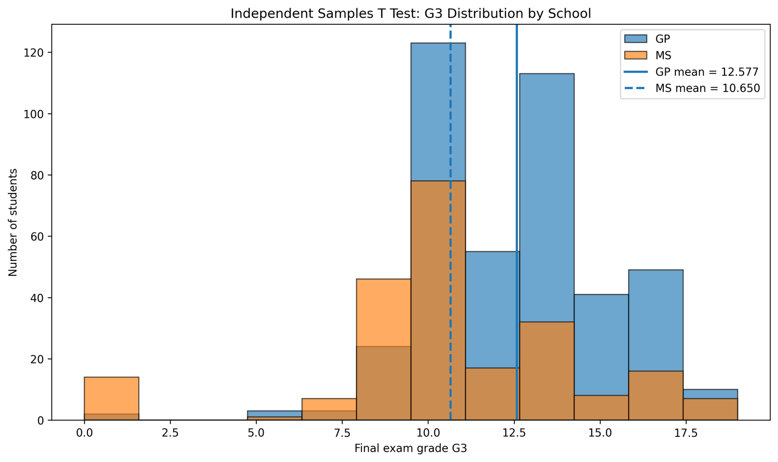
This histogram shows that the overall GP distribution is shifted to the right of the MS distribution. That means GP students tend to have higher final grades than MS students. The chart legend displays the exact group means: GP mean = 12.577 and MS mean = 10.650.
The plot also shows that the MS group has a wider spread, which matches the larger standard deviation reported later. Even though the two distributions overlap, the center of GP is clearly higher, which visually supports the significant t test result.
Python Chart 2: Group Means with 95% Confidence Intervals
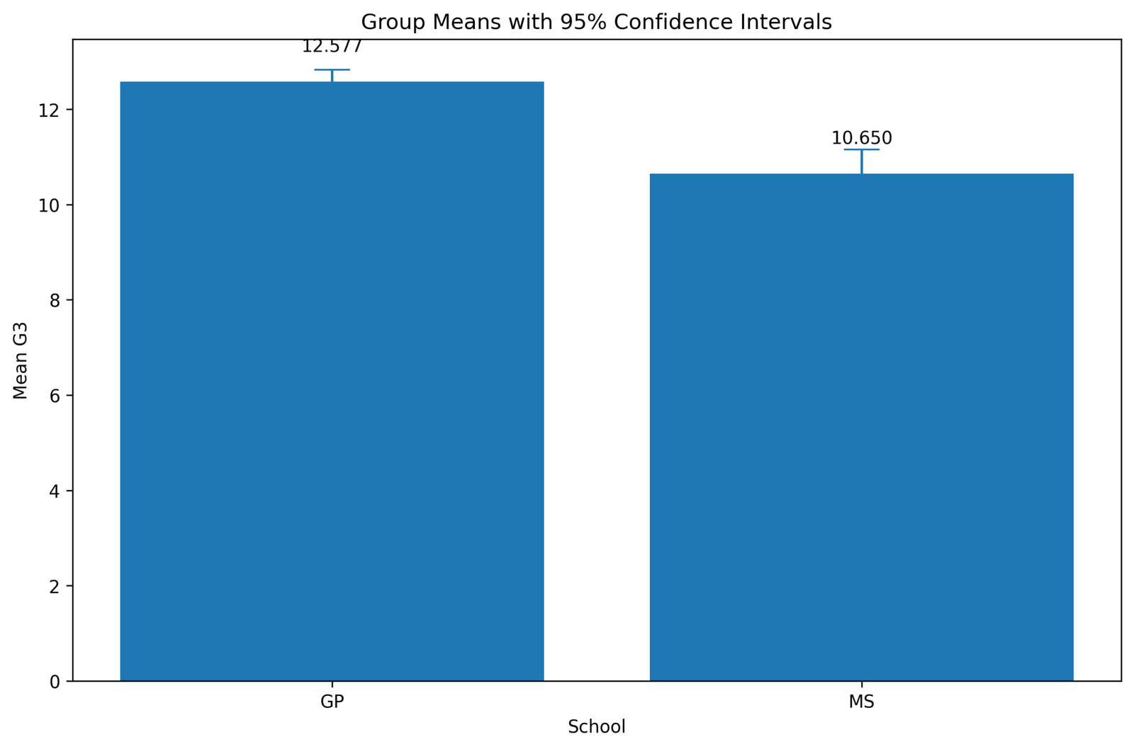
This chart emphasizes the mean difference directly. The GP bar is clearly taller than the MS bar, and the numeric labels repeat the exact means. The confidence intervals around the group means help show sampling uncertainty.
Because the group means are separated by nearly two points, the chart communicates that the group difference is not a tiny statistical artifact. It is visually substantial and consistent with the inferential result.
Python Chart 3: Mean Difference Confidence Interval
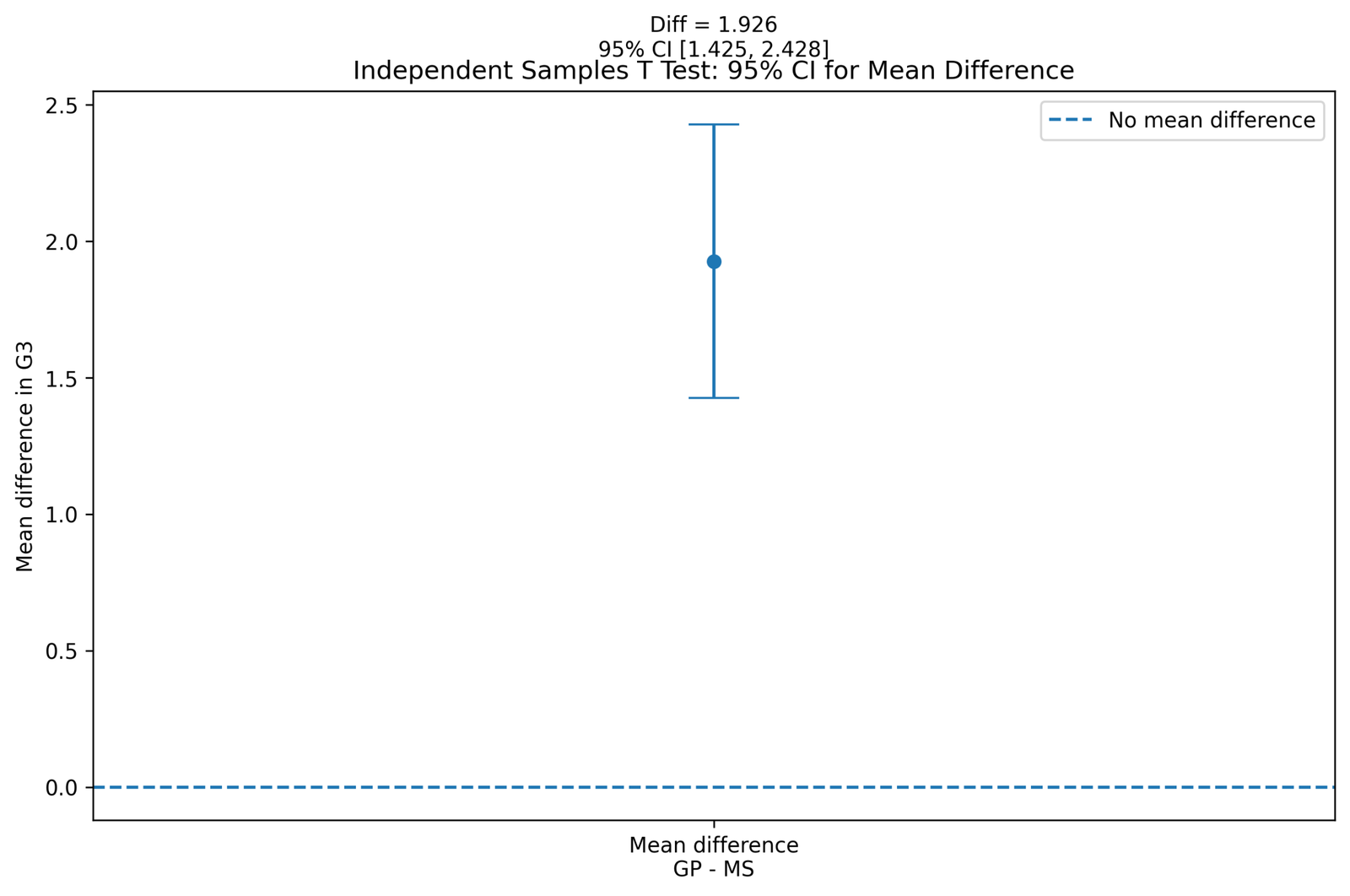
This is one of the most important charts in the entire analysis. It shows the estimated mean difference of 1.926 with a 95% CI from 1.425 to 2.428. The dashed horizontal reference line at zero represents “no mean difference.”
Because the entire interval is above zero, the conclusion is clear: GP has a significantly higher mean G3 score than MS. Confidence-interval interpretation is often more informative than a p-value alone because it shows both the direction and plausible magnitude of the difference.
Python Chart 4: t Statistic on Student’s t Distribution
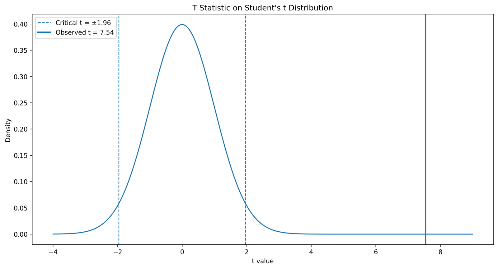
This chart places the observed test statistic t = 7.54 on the t distribution. The critical values for a two-tailed 5% test are shown around ±1.96. The observed t value is far beyond the critical region.
This means the observed group difference is much larger than what we would expect under the null hypothesis of equal means. Graphically, the chart confirms why the p-value is extremely small.
Python Chart 5: G3 Boxplot by Group
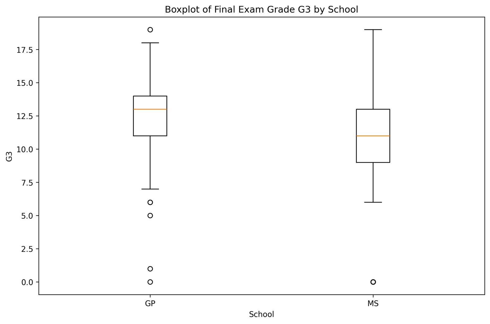
The boxplot provides a clean summary of group distributions. The median of GP is higher than the median of MS, which agrees with the mean-based t test result. Both groups show some lower-end outliers, including zero scores, but the central location of GP remains higher.
The MS box also appears more spread out, which fits the larger standard deviation. This chart is particularly helpful for spotting skewness, outliers and group spread at a glance.
Python Chart 6: Group Standard Deviation Comparison
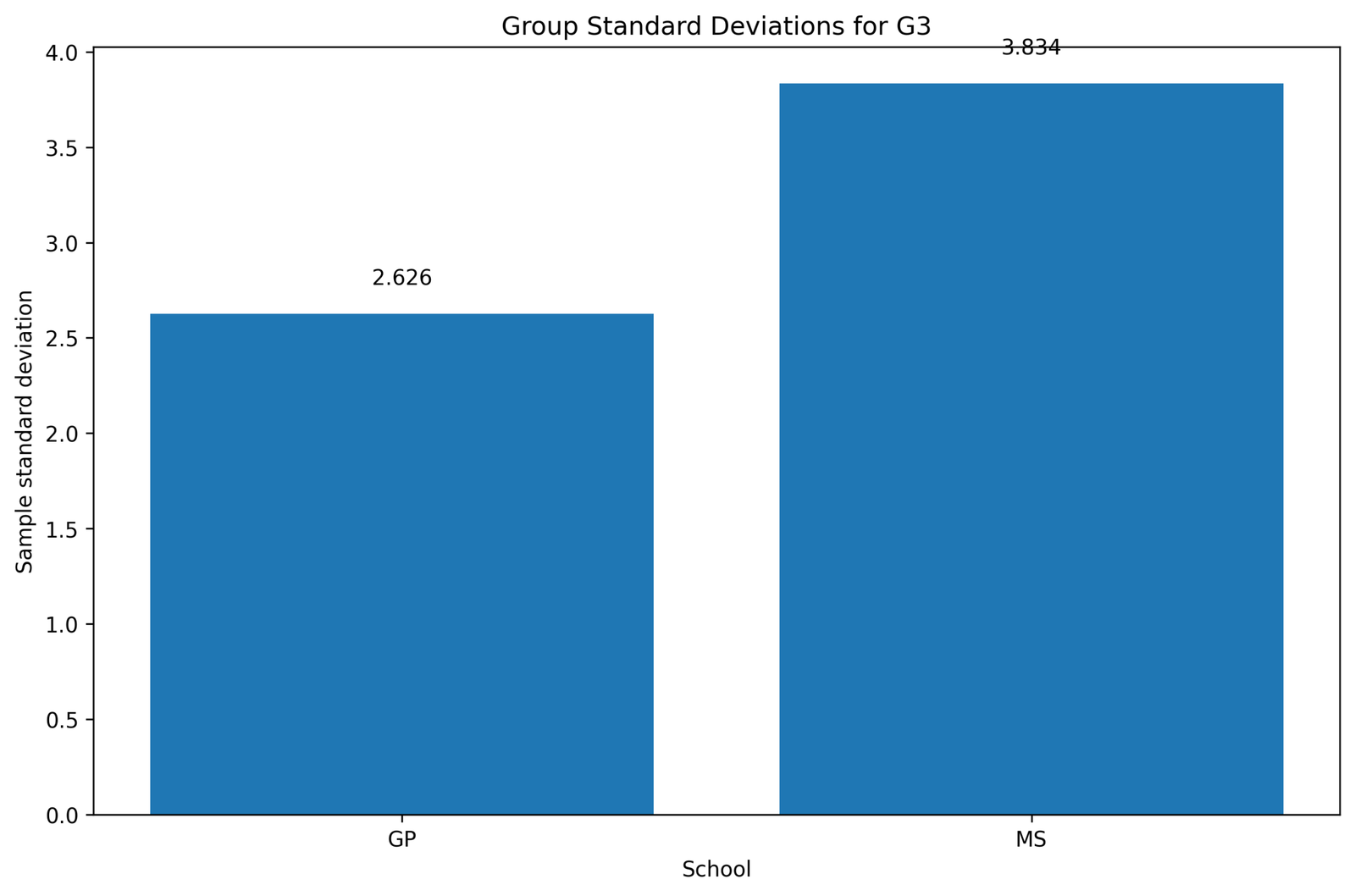
This chart shows that the standard deviation for GP is 2.626, while the standard deviation for MS is 3.834. That means scores in MS are more variable.
This matters for assumption checking because the equal-variances version of the t test works best when group variances are reasonably similar. The difference in SDs suggests that Levene’s test should be reported when available, but it does not overturn the core conclusion of the analysis.
Python Chart 7: Mean G3 by Study Time within Group
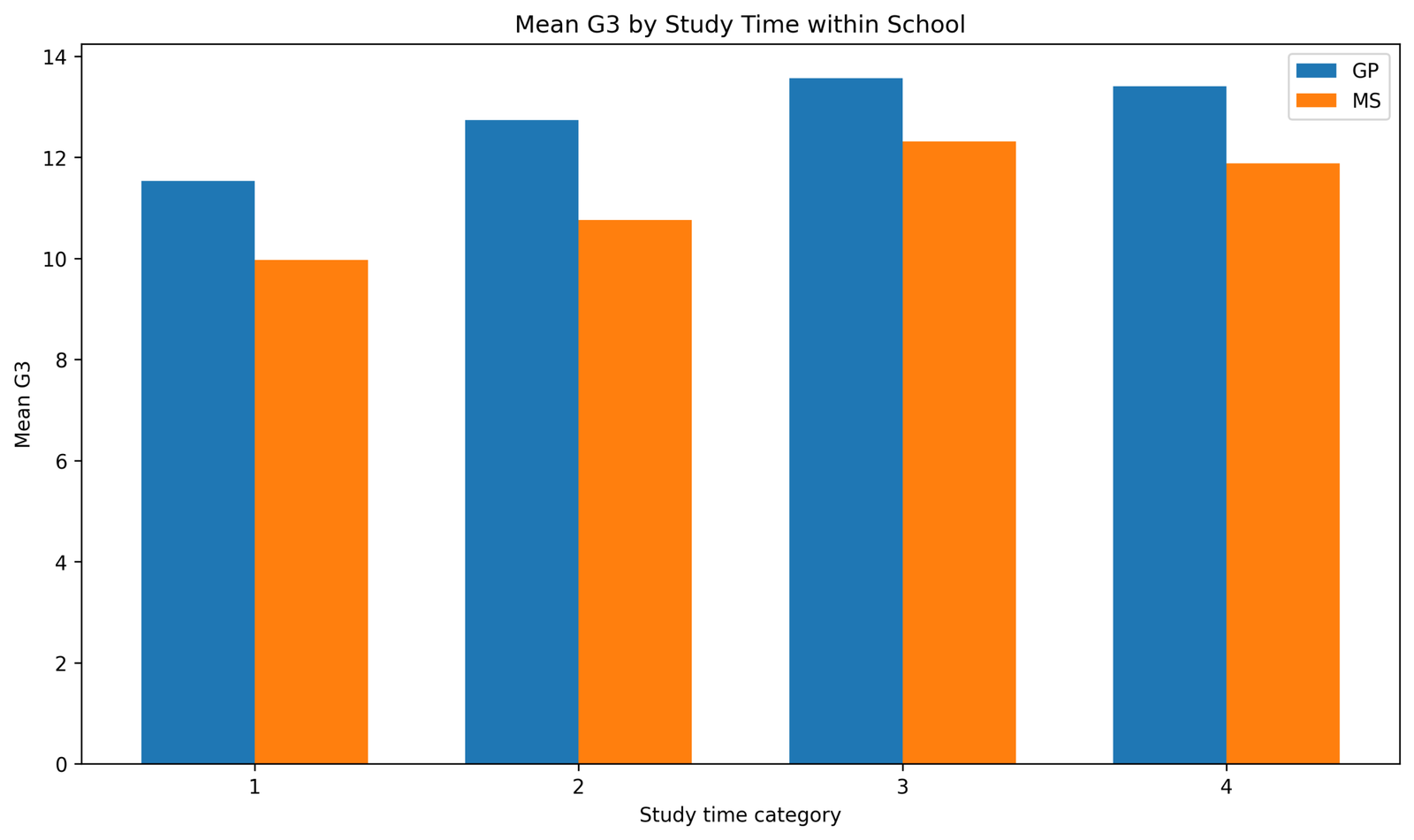
This chart adds useful context. Across all study-time categories, GP tends to maintain higher mean G3 scores than MS. In other words, the GP advantage is not limited to only one study-time category.
This does not replace a factorial model, but it is a strong descriptive sign that the group difference is broadly consistent across subgroups. It strengthens the practical interpretation of the mean difference.
R Chart-by-Chart Validation
The R chart set validates the same findings using a different software workflow. This cross-software agreement is important because it shows the result is not dependent on one package.
R Chart 1: G3 Distribution by Group
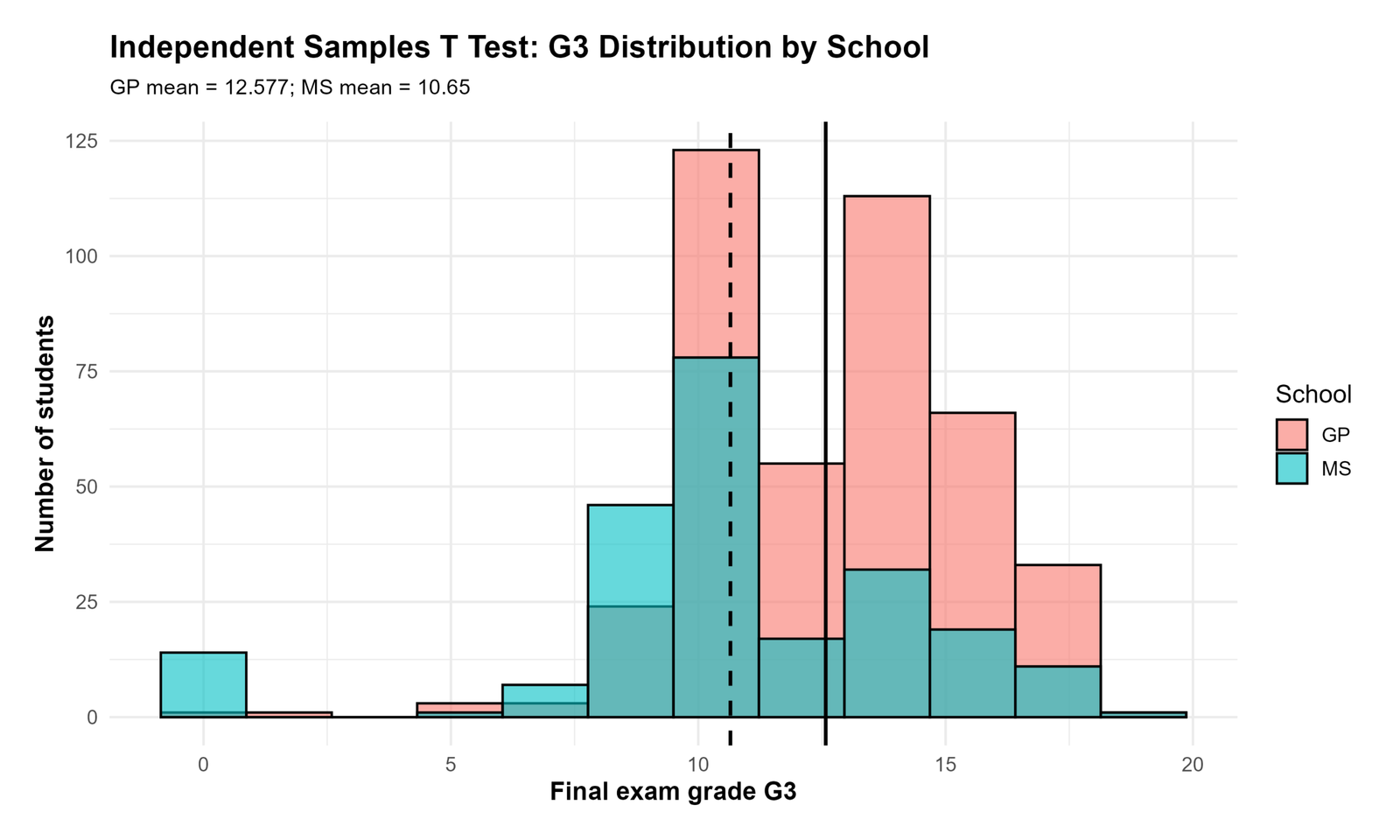
The R distribution chart confirms the same pattern seen in Python: GP scores are centered at a higher level than MS scores. Although both groups share some overlap, the distribution centers are clearly separated.
This supports the main conclusion that the difference is not random noise. It is visible in the raw score structure.
R Chart 2: Group Means with 95% Confidence Intervals
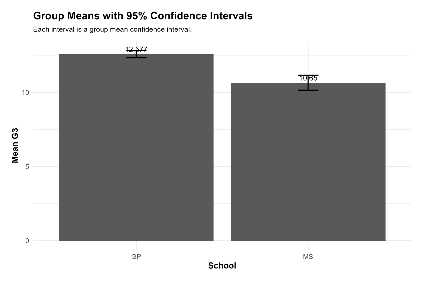
The R bar chart again shows GP with a higher average G3 than MS. The confidence intervals reinforce that the GP mean is clearly above the MS mean.
When two different programs draw the same picture from the same data, confidence in the interpretation increases.
R Chart 3: Mean Difference Confidence Interval
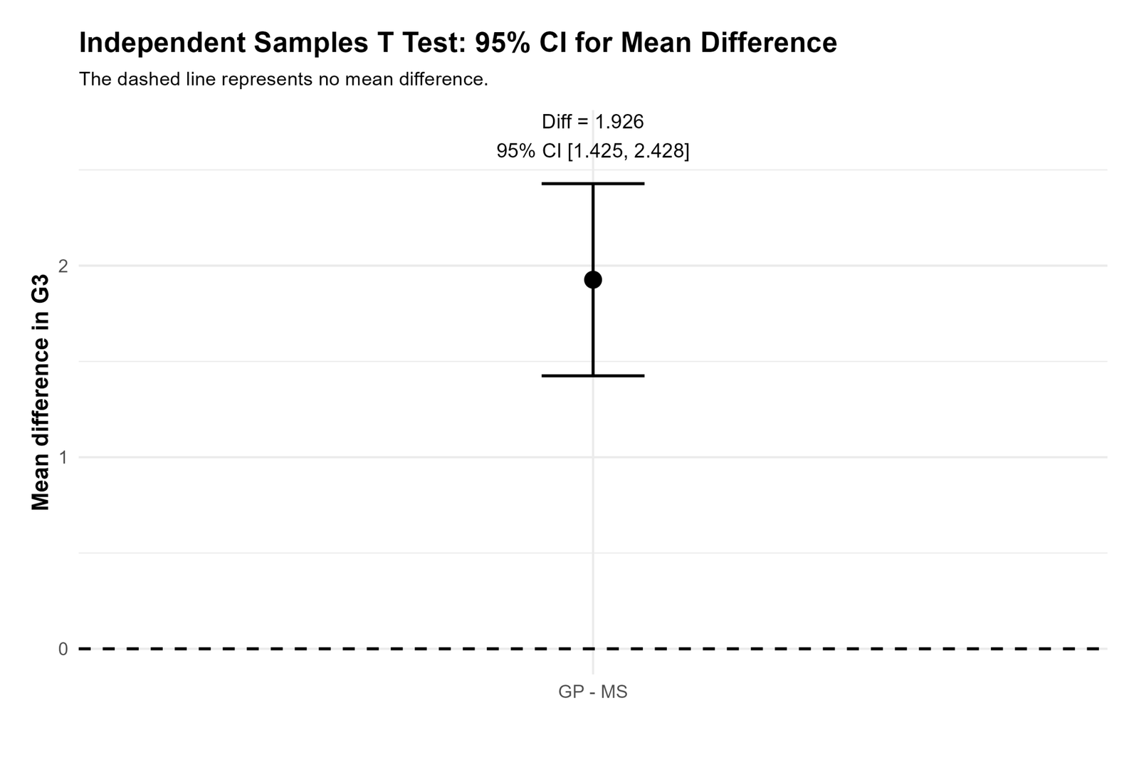
This chart repeats the crucial inferential message: the mean difference is positive and the 95% interval stays above zero. That is direct visual evidence that GP students scored significantly higher.
Confidence intervals are especially helpful because they provide more than a yes/no decision. They show how large the true difference is likely to be.
R Chart 4: t Statistic on Student’s t Distribution
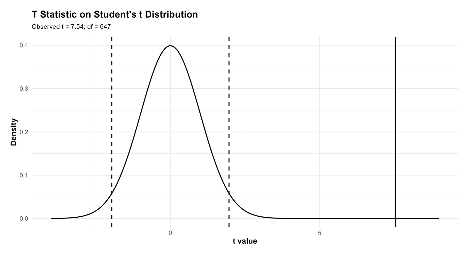
This R chart explicitly labels Observed t = 7.54 and df = 647. Those values match the Python-based interpretation and confirm that the same inferential conclusion was reached in R.
Because the observed t statistic lies far beyond the critical region, the null hypothesis of equal means is decisively rejected.
R Chart 5: G3 Boxplot by Group
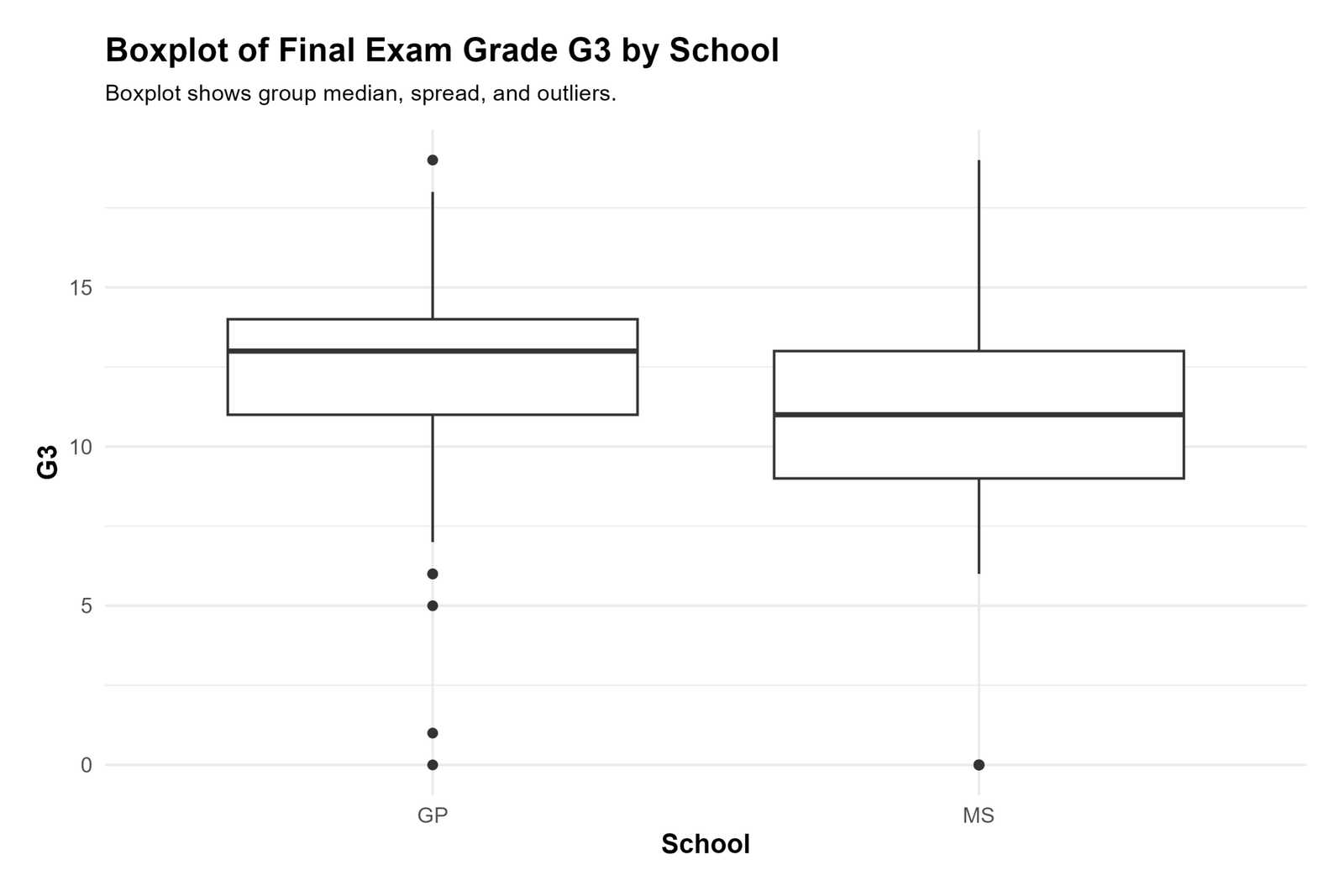
The R boxplot confirms the same structure observed earlier: higher central tendency in GP and greater spread in MS. The lower-end outliers do not erase the consistent upward shift of GP.
That is why robust descriptive visuals and formal hypothesis tests are best interpreted together.
R Chart 6: Group Standard Deviation Comparison
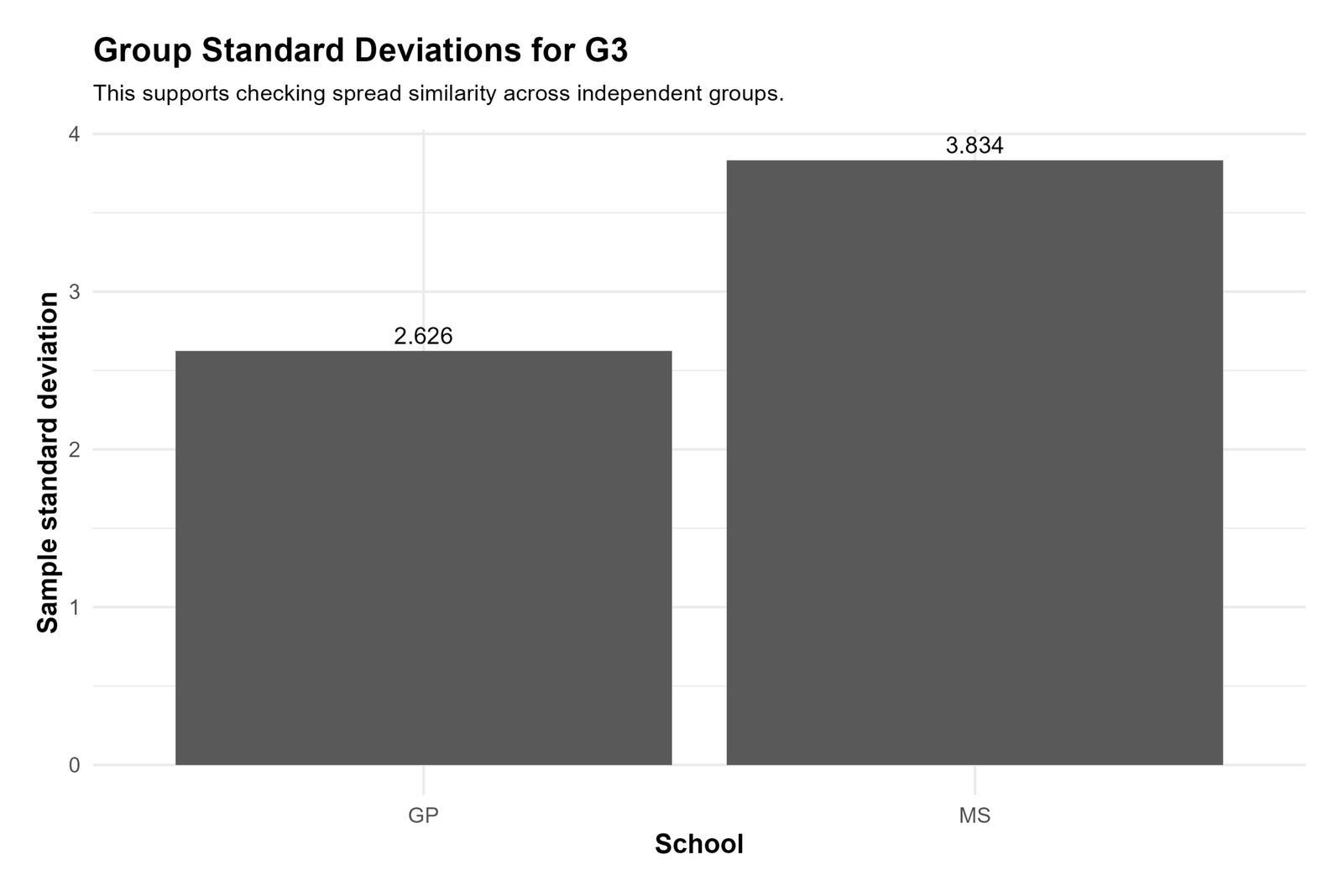
The R standard deviation chart again highlights a larger spread in MS. This repeated pattern is useful for discussing the homogeneity of variances assumption and the relevance of Levene’s test.
Even if the assumption is imperfect, the large sample and sizeable mean difference make the main conclusion robust.
R Chart 7: Mean G3 by Study Time within Group
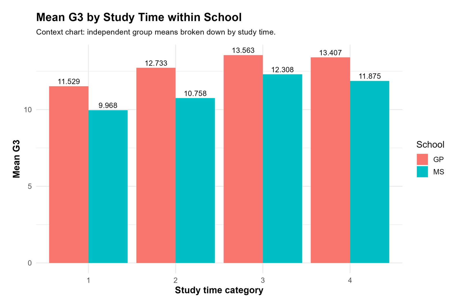
The R study-time chart tells the same practical story as the Python version. GP tends to score higher across study-time levels, which suggests the school-level difference is fairly stable across these descriptive subgroups.
This cross-check is useful for interpretation because it shows that the GP advantage is not an artifact from only one subgroup.
SPSS, R, Python and Excel Workflows for the Independent Samples T Test
SPSS Workflow
| Step | SPSS Menu or Syntax | Purpose |
|---|---|---|
| Open dataset | File > Open > Data | Load the student dataset. |
| Select test | Analyze > Compare Means > Independent-Samples T Test | Choose the correct two-group mean comparison procedure. |
| Test variable | G3 | Dependent variable. |
| Grouping variable | school | Define groups as GP and MS. |
| Run test | OK | Obtain Group Statistics and the Independent Samples Test table. |
| Interpret output | Check t, df, p, mean difference and CI | Make the inferential decision. |
R Workflow
| Step | R Action | Purpose |
|---|---|---|
| Read data | read.csv() | Load the dataset. |
| Convert groups | factor() | Ensure school is treated as a grouping factor. |
| Run t test | t.test(G3 ~ school, data = df, var.equal = TRUE) | Fit the independent t test. |
| Descriptives | aggregate() or dplyr | Get means, SDs and n by group. |
| Effect size | Manual formula or effsize | Calculate Cohen’s d. |
Python Workflow
| Step | Python Action | Purpose |
|---|---|---|
| Read data | pandas.read_csv() | Load the dataset. |
| Subset groups | Filter GP and MS | Create the two independent samples. |
| Run test | scipy.stats.ttest_ind() | Calculate the t statistic and p-value. |
| Descriptive statistics | groupby().agg() | Get group means and SDs. |
| Visualization | matplotlib | Create the histogram, CI, boxplot and SD comparison charts. |
Excel Workflow
| Excel Task | Formula or Tool | Purpose |
|---|---|---|
| Separate groups | Filter school into GP and MS columns | Prepare the two independent samples. |
| Get means and SDs | AVERAGE(), STDEV.S() | Compute group descriptives. |
| Run test | Data Analysis ToolPak > t-Test: Two-Sample Assuming Equal Variances | Obtain t, p and confidence information. |
| Interpret results | Compare p-value with alpha | Decide whether the means differ significantly. |
| Visualize | Insert charts | Create bar charts, boxplots and distribution charts for reporting. |
Code Blocks for the Independent Samples T Test
SPSS Syntax
* Independent Samples T Test for G3 by school.
* Groups: GP and MS.

TITLE "Independent Samples T Test: G3 by School".

T-TEST GROUPS=school('GP' 'MS')
  /VARIABLES=G3
  /CRITERIA=CI(.95).

* Optional descriptive statistics.
MEANS TABLES=G3 BY school
  /CELLS MEAN COUNT STDDEV SEMEAN.

OUTPUT EXPORT
  /CONTENTS EXPORT=VISIBLE
  /PDF DOCUMENTFILE="Independent-Samples-T-Test-SPSS-Output.pdf".
Python Code
import pandas as pd
import numpy as np
from scipy import stats

df = pd.read_csv("dataset.csv")

# Keep needed columns
data = df[["school", "G3", "studytime"]].copy()
data["G3"] = pd.to_numeric(data["G3"], errors="coerce")
data = data.dropna(subset=["school", "G3"])

gp = data.loc[data["school"] == "GP", "G3"]
ms = data.loc[data["school"] == "MS", "G3"]

# Descriptive statistics
summary = data.groupby("school")["G3"].agg(["count", "mean", "std"])
print(summary)

# Independent samples t test
t_stat, p_val = stats.ttest_ind(gp, ms, equal_var=True)
print("t =", t_stat)
print("p =", p_val)

# Mean difference and CI
n1, n2 = len(gp), len(ms)
m1, m2 = gp.mean(), ms.mean()
s1, s2 = gp.std(ddof=1), ms.std(ddof=1)

sp = np.sqrt(((n1 - 1) * s1**2 + (n2 - 1) * s2**2) / (n1 + n2 - 2))
se = sp * np.sqrt(1/n1 + 1/n2)
dfree = n1 + n2 - 2
crit = stats.t.ppf(0.975, dfree)

mean_diff = m1 - m2
ci_low = mean_diff - crit * se
ci_high = mean_diff + crit * se

cohens_d = mean_diff / sp

print("Mean difference =", mean_diff)
print("95% CI =", (ci_low, ci_high))
print("Cohen's d =", cohens_d)
R Code
# Independent Samples T Test for G3 by school

df <- read.csv("dataset.csv")

df$school <- as.factor(df$school)
df$G3 <- as.numeric(df$G3)

df_model <- na.omit(df[, c("school", "G3", "studytime")])

# Descriptive statistics
aggregate(G3 ~ school, data = df_model,
          FUN = function(x) c(n = length(x), mean = mean(x), sd = sd(x)))

# T test
result <- t.test(G3 ~ school, data = df_model, var.equal = TRUE)
print(result)

# Effect size
gp <- df_model$G3[df_model$school == "GP"]
ms <- df_model$G3[df_model$school == "MS"]

n1 <- length(gp)
n2 <- length(ms)
m1 <- mean(gp)
m2 <- mean(ms)
s1 <- sd(gp)
s2 <- sd(ms)

sp <- sqrt(((n1 - 1) * s1^2 + (n2 - 1) * s2^2) / (n1 + n2 - 2))
d <- (m1 - m2) / sp

cat("Cohen's d =", d, "\n")
Excel Steps
Step 1:
Place GP G3 values in one column and MS G3 values in another.

Step 2:
Calculate group means:
=AVERAGE(range)

Step 3:
Calculate group standard deviations:
=STDEV.S(range)

Step 4:
Open Data Analysis ToolPak.
Choose: t-Test: Two-Sample Assuming Equal Variances

Step 5:
Select GP and MS ranges.
Set Hypothesized Mean Difference = 0
Alpha = 0.05

Step 6:
Interpret:
- If p < .05, reject the null hypothesis.
- Check the mean difference and t statistic.
- Report the confidence interval if available.

Step 7:
Create charts:
- Histogram by group
- Mean comparison chart
- Boxplot
- Standard deviation comparison
APA Reporting for the Independent Samples T Test
Here is a ready-to-use APA-style reporting example for this analysis:
An independent-samples t test was conducted to compare final exam grade (G3) between GP and MS students. GP students (M = 12.58, SD = 2.63) scored significantly higher than MS students (M = 10.65, SD = 3.83), t(647) = 7.54, p < .001, with a mean difference of 1.93, 95% CI [1.43, 2.43]. The effect size was medium (Cohen’s d = 0.62).
If your instructor or journal requires it, you can also add a note about the variance assumption and Levene’s test when the SPSS table is available.
Common Mistakes in the Independent Samples T Test
| Mistake | Why It Is a Problem | Correct Practice |
|---|---|---|
| Using paired data with an independent t test | The test assumes unrelated groups. | Use a paired t test for repeated or matched observations. |
| Reporting only p-value | You lose information about magnitude and direction. | Report means, SDs, mean difference, CI and effect size. |
| Ignoring variance differences | Equal-variances assumptions may be questionable. | Check Levene’s test or use Welch’s version if needed. |
| Calling significance “importance” | A statistically significant result may still be practically small. | Interpret significance together with effect size. |
| Skipping visual checks | Outliers and spread patterns can be missed. | Always review histograms and boxplots. |
When to Use the Independent Samples T Test
Use the Independent Samples T Test when:
- You have two unrelated groups.
- Your outcome variable is continuous.
- You want to test whether the group means differ.
- The assumptions are at least reasonably acceptable.
Examples include comparing:
- exam scores between two schools,
- blood pressure between treatment and control groups,
- income between two employment categories,
- customer ratings between two service models.
Downloads and Resources
Download SPSS Syntax
Replace this placeholder with your hosted SPSS syntax file URL.
Download Python Script
Replace this placeholder with your hosted Python file URL.
Download R Script
Replace this placeholder with your hosted R file URL.
Download Excel Template
Replace this placeholder with your hosted Excel file URL.
Frequently Asked Questions
What does the Independent Samples T Test tell us?
It tells us whether the average value of a continuous outcome differs significantly between two unrelated groups. In this example, it shows that GP students have a higher average G3 score than MS students.
What is the null hypothesis for the Independent Samples T Test?
The null hypothesis states that the two population means are equal. Here, it means the average G3 score in GP is equal to the average G3 score in MS.
How do I interpret t(647) = 7.54, p < .001?
This means the observed difference between the group means is very large relative to sampling error, and the probability of seeing such a difference under the null hypothesis is extremely small. Therefore, the mean difference is statistically significant.
Why is the confidence interval important?
The confidence interval shows the plausible range for the true mean difference. Here, the 95% CI is [1.425, 2.428], so we can be reasonably confident that GP really scores higher than MS by about 1.4 to 2.4 points on average.
What does Cohen’s d = 0.62 mean?
It means the size of the group difference is moderate. The difference is not only statistically significant, but also practically meaningful.
Do I always need Levene’s test?
You should usually report it when using the standard independent t test, because it checks whether the group variances are similar. If variances differ notably, Welch’s t test is often preferred.
Can I use the Independent Samples T Test with more than two groups?
No. If you have more than two independent groups, you usually need ANOVA instead of the Independent Samples T Test.

