Sampling Distributions, Standard Error and Normal Approximation
Central Limit Theorem explains why sample means become more stable, more normally shaped and closer to the population mean as sample size increases. This complete guide explains the Central Limit Theorem formula, sampling distribution of the mean, standard error, confidence interval coverage, Q-Q plot interpretation, SPSS output, R workflow, Python workflow and Excel method using the student-por.csv dataset.
Google AdSense top placement reserved here
Quick Answer: Central Limit Theorem Result
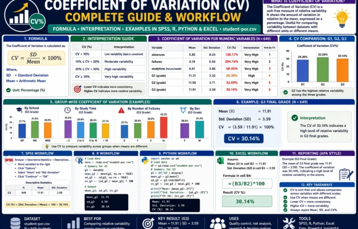
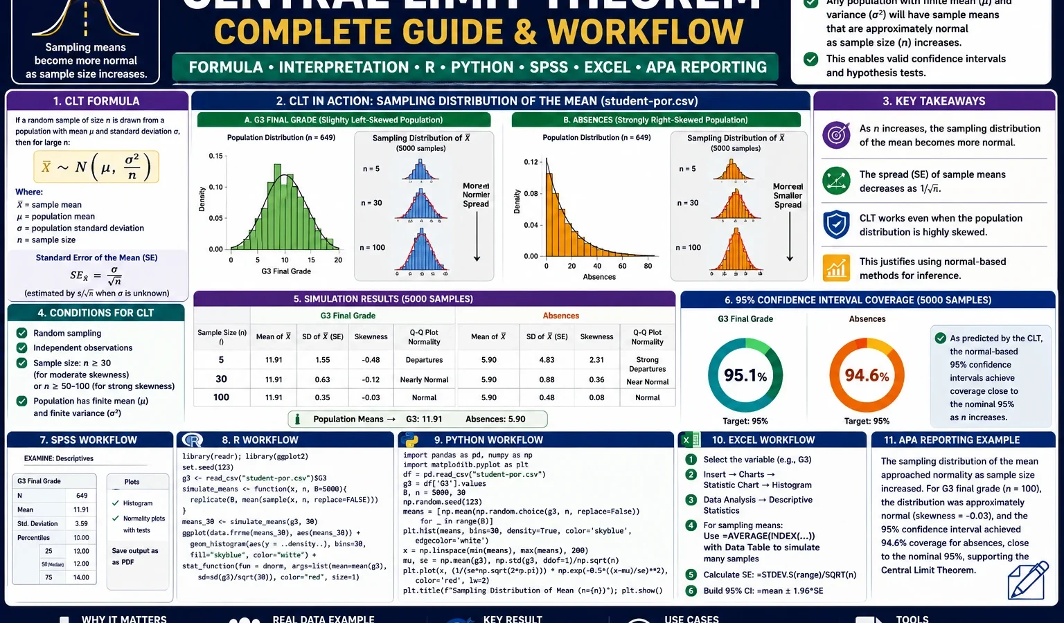
The Central Limit Theorem was demonstrated using the G3 final grade and absences variables from the student-por.csv dataset. The original G3 population had n = 649, mean = 11.9060 and SD = 3.2307. After repeated sampling, the distribution of sample means became narrower as sample size increased. For G3, the simulated standard deviation of sample means dropped from about 1.4562 at n = 5 to about 0.3238 at n = 100.
Final report sentence: The Central Limit Theorem simulation showed that the sampling distribution of the mean became more stable as sample size increased. For G3 final grade, the population mean was 11.9060 and the population standard deviation was 3.2307. The simulated standard deviation of G3 sample means decreased from 1.4562 at n = 5 to 0.3238 at n = 100, closely matching the theoretical standard error formula SE = σ / √n. Therefore, larger samples produced sample means that were more tightly centered around the population mean.
Important interpretation note: The Central Limit Theorem does not say that the original raw data must be normal. It says that the distribution of sample means tends to become approximately normal as sample size increases, especially when sampling is random and observations are independent.
Table of Contents
- What Is the Central Limit Theorem?
- Central Limit Theorem Formula
- Dataset and Clean SPSS-Ready Files Used
- Verified SPSS, R and Python Results
- Python Charts and Interpretation
- R Validation Charts
- How to Run CLT in Python, R, SPSS and Excel
- How to Report the Central Limit Theorem Result
- Common Mistakes
- Download SPSS Output
- FAQs
What Is the Central Limit Theorem?
The Central Limit Theorem is one of the most important ideas in statistics. It explains why the sample mean is so useful in real data analysis. When repeated random samples are taken from a population, the means of those samples form their own distribution. This new distribution is called the sampling distribution of the mean.
The Central Limit Theorem says that as the sample size becomes larger, the sampling distribution of the mean becomes approximately normal, even when the original population is not perfectly normal. This is why many statistical methods can use normal-based reasoning for sample means, confidence intervals and hypothesis tests.
In this worked example, G3 final grade is used as the main population variable. The original G3 distribution is not perfectly normal because it includes low-grade values and a visible left-tail pattern. The absences variable is even more extreme because it is strongly right-skewed. However, when repeated sample means are generated, the sampling distributions become smoother and more normal-looking as sample size increases.
Practical meaning: Individual observations may be irregular, skewed or noisy, but averages based on larger random samples are usually more stable. That is the practical reason the Central Limit Theorem supports confidence intervals, standard errors, z tests, t tests and many regression-based procedures.
For related assumption-checking and normality topics, see the Q-Q Plot Normality Check, Shapiro-Wilk Test, Kolmogorov-Smirnov Test, DAgostino Pearson Test and One-Sample Z Test.
Central Limit Theorem Formula
The main Central Limit Theorem formula used in this guide is the standard error of the sample mean:
SE of sample mean = σ / √nWhere:
| Symbol | Meaning | In this example |
|---|---|---|
| SE | Standard error of the sample mean | The spread of repeated sample means. |
| σ | Population standard deviation | For G3, approximately 3.2307. |
| n | Sample size | 5, 10, 30, 50 and 100 were simulated. |
| √n | Square root of sample size | As n grows, √n grows, so standard error becomes smaller. |
The formula explains the visual pattern in the charts. When n = 5, sample means vary more widely. When n = 100, sample means are much closer to the population mean. The standard error decreases because the population standard deviation is divided by the square root of the sample size.
Formula using the G3 result: For G3, the population standard deviation is about 3.2307. At n = 100, the theoretical standard error is about 3.2307 / √100 = 0.3231, which closely matches the simulated standard deviation of sample means, about 0.3238.
Dataset and Clean SPSS-Ready Files Used
This Central Limit Theorem example uses the student-por.csv student performance dataset. The main variable is G3 final grade, and the second demonstration variable is absences. G3 shows how sample means stabilize for a grade variable, while absences shows that the Central Limit Theorem can still work even when the original variable is highly skewed.
Important SPSS workflow rule: Python was used first to create clean SPSS-ready files. SPSS then imported those clean files instead of reading the raw dataset directly. This prevents delimiter problems, wrong variable types and column-mapping errors.
| Item | File or value | Explanation |
|---|---|---|
| Input cleaned data | spss_ready_data.csv | Cleaned dataset already available in the topic folder. |
| Python file for SPSS original data | clt_clean_data_for_spss.csv | Clean original dataset exported for SPSS. |
| Python file for SPSS sampling means | clt_sampling_means_wide_for_spss.csv | Wide-format sampling-distribution file exported for SPSS. |
| Main variable | G3 | Final grade used as the main Central Limit Theorem demonstration variable. |
| Second variable | absences | Right-skewed variable used to show that CLT still works with skewed original data. |
| Population size | 649 | Total valid cases in the cleaned dataset. |
| Topic folder | D:\DATA ANALYSIS\A Basic Descriptive Statistics Guides\Central Limit Theorem | All R, Python and SPSS outputs are saved inside this topic folder. |
External dataset source: UCI Machine Learning Repository: Student Performance dataset.
Google AdSense middle placement reserved here
Verified SPSS, R and Python Results
The Central Limit Theorem workflow was reproduced in Python, R and SPSS. Python generated the clean SPSS-ready files and charts. R produced independent validation charts. SPSS imported the clean files and produced descriptive statistics, frequency tables, normality checks and sampling-distribution summaries.
Original Data Check
| Variable | N | Minimum | Maximum | Mean | Standard deviation | Interpretation |
|---|---|---|---|---|---|---|
| G1 first period grade | 649 | 0.00 | 19.00 | 11.3991 | 2.74527 | First period grade distribution. |
| G2 second period grade | 649 | 0.00 | 19.00 | 11.5701 | 2.91364 | Second period grade distribution. |
| G3 final grade | 649 | 0.00 | 19.00 | 11.9060 | 3.23066 | Main variable for the CLT demonstration. |
| Absences | 649 | 0.00 | 32.00 | 3.6595 | 4.64076 | Right-skewed variable used as a second CLT demonstration. |
Original Distribution Shape
| Variable | Mean | Median | SD | Skewness | Kurtosis | Shapiro-Wilk W | Decision |
|---|---|---|---|---|---|---|---|
| G3 final grade | 11.9060 | 12.0000 | 3.23066 | -0.913 | 2.712 | 0.926, p < .001 | Reject normality for raw G3. |
| Absences | 3.6595 | 2.0000 | 4.64076 | 2.021 | 5.781 | 0.772, p < .001 | Reject normality for raw absences. |
Sampling Distribution of G3 Sample Means
The main Central Limit Theorem result is visible in the G3 sample-mean table. The mean of repeated sample means stays close to the population mean, while the standard deviation of sample means becomes smaller as sample size increases.
| Sample size | Mean of sample means | SD of sample means | Skewness | Kurtosis | Interpretation |
|---|---|---|---|---|---|
| n = 5 | 11.91736 | 1.45621 | -0.376 | 0.534 | Sample means are still fairly spread out. |
| n = 10 | 11.90094 | 1.01219 | -0.345 | 0.271 | Spread decreases compared with n = 5. |
| n = 30 | 11.90086 | 0.58825 | -0.169 | 0.114 | Distribution is much narrower and more normal-looking. |
| n = 50 | 11.91424 | 0.45920 | -0.090 | -0.019 | Sample means are closely centered around the population mean. |
| n = 100 | 11.90284 | 0.32382 | -0.134 | -0.004 | Very stable sampling distribution. |
Sampling Distribution of Absences Sample Means
The absences variable is strongly right-skewed in the raw data, but the sample means still become more stable as sample size increases. This is a strong practical demonstration of the Central Limit Theorem.
| Sample size | Mean of sample means | SD of sample means | Skewness | Kurtosis | Interpretation |
|---|---|---|---|---|---|
| n = 5 | 3.67144 | 2.05738 | 0.928 | 1.261 | Still visibly skewed at a very small sample size. |
| n = 10 | 3.64144 | 1.46683 | 0.667 | 0.651 | Skewness begins to reduce. |
| n = 30 | 3.65429 | 0.84667 | 0.364 | 0.154 | Sample means become more bell-shaped. |
| n = 50 | 3.66823 | 0.65718 | 0.280 | 0.086 | Sampling distribution is more stable. |
| n = 100 | 3.65806 | 0.46941 | 0.199 | 0.002 | Sample means are much closer to a normal pattern. |
SPSS Output Transcript
Original G3 transcript: Valid N = 649, mean = 11.9060, median = 12.0000, standard deviation = 3.23066, variance = 10.437, skewness = -0.913, kurtosis = 2.712, minimum = 0, maximum = 19, Q1 = 10, Q3 = 14. Shapiro-Wilk normality test for raw G3: W = 0.926, p < .001.
Original absences transcript: Valid N = 649, mean = 3.6595, median = 2.0000, standard deviation = 4.64076, variance = 21.537, skewness = 2.021, kurtosis = 5.781, minimum = 0, maximum = 32, Q1 = 0, Q3 = 6. Shapiro-Wilk normality test for raw absences: W = 0.772, p < .001.
Sampling-distribution transcript: G3 sample means remained centered near 11.9060, while their standard deviation decreased as sample size increased: 1.4562 at n = 5, 1.0122 at n = 10, 0.5882 at n = 30, 0.4592 at n = 50 and 0.3238 at n = 100.
Python Charts and Interpretation
1. Raw G3 Population Distribution

This chart shows the original G3 final-grade population distribution. The mean is about 11.91 and the median is 12.00. The distribution is not perfectly normal, but it is concentrated around the middle grade range. This chart is important because the Central Limit Theorem begins with the original population distribution before repeated sampling is performed.
2. Sampling Distribution of the Mean for G3

This is the core Central Limit Theorem chart. At n = 5, the sample means are spread more widely. At n = 30, the distribution is already much more stable and bell-shaped. At n = 100, sample means cluster tightly around the population mean. This visual pattern matches the standard error formula.
3. Standard Error Decreases as Sample Size Increases

The line chart shows that the simulated standard deviation of sample means closely follows the theoretical standard error σ / √n. This means the simulation is working correctly. As sample size increases, the standard error becomes smaller, so the sample mean becomes a more precise estimate of the population mean.
4. Raw Absences Distribution Is Right-Skewed

The raw absences variable is strongly right-skewed. Many students have zero or very few absences, while a smaller number have large absence values. The mean is higher than the median because the right-tail values pull the average upward. This chart is useful because it shows that the Central Limit Theorem is not limited to perfectly normal original data.
5. Central Limit Theorem with Skewed Absences Data

This chart demonstrates the practical power of the Central Limit Theorem. Even though the original absences distribution is highly skewed, the sampling distribution of the mean becomes more bell-shaped as sample size increases. At n = 5, the distribution still has visible skewness. At n = 50 and n = 100, the sample means are much more stable and closer to normal.
6. Q-Q Plots of G3 Sample Means

The Q-Q plots confirm what the histograms show. At smaller sample sizes, the tails depart more from the reference line. As sample size increases, the plotted points move closer to the line, meaning the sampling distribution becomes more normal. This is direct visual evidence for the Central Limit Theorem.
7. 95% Confidence Interval Coverage for G3

This chart connects the Central Limit Theorem with confidence intervals. The target coverage is 0.95. Smaller sample sizes show lower coverage, while larger samples move closer to the target. This is why normal-based confidence intervals usually perform better when sample size is larger and the sampling distribution is more stable.
8. Sample Mean Stabilizes as Sample Size Grows

This line chart shows convergence. Early sample means can jump up and down because small samples are unstable. As sample size grows, the sample mean fluctuates less and stays closer to the population mean. This is the same idea behind using larger samples for more reliable statistical estimates.
9. Population Distribution vs Sampling Distribution

This chart compares the raw population distribution with the sampling distribution. The population distribution is wider because it contains individual grades. The sampling distribution of means is narrower because each value is an average of many observations. This distinction is essential for understanding standard error.
R Validation Charts for the Central Limit Theorem
The R workflow produced matching validation charts. These charts confirm that the same Central Limit Theorem pattern appears outside Python and SPSS.


How to Run the Central Limit Theorem in Python, R, SPSS and Excel
Central Limit Theorem in Python
The Python workflow uses the cleaned dataset, saves charts, creates the clean SPSS import file and creates the sampling-means file used by SPSS.
import os
import numpy as np
import pandas as pd
import matplotlib.pyplot as plt
from scipy import stats

base_dir = r"D:\DATA ANALYSIS\A Basic Descriptive Statistics Guides\Central Limit Theorem"
input_clean_csv = os.path.join(base_dir, "spss_ready_data.csv")

python_dir = os.path.join(base_dir, "Python")
spss_dir = os.path.join(base_dir, "SPSS")
os.makedirs(python_dir, exist_ok=True)
os.makedirs(spss_dir, exist_ok=True)

df = pd.read_csv(input_clean_csv)

required = ["school", "sex", "age", "studytime", "failures", "absences", "G1", "G2", "G3"]
missing = [c for c in required if c not in df.columns]
if missing:
    raise ValueError(f"Missing required columns: {missing}")

clean = df[required].copy()
for col in ["age", "studytime", "failures", "absences", "G1", "G2", "G3"]:
    clean[col] = pd.to_numeric(clean[col], errors="coerce")

clean = clean.dropna(subset=["G3", "absences"]).reset_index(drop=True)
clean.insert(0, "case_id", np.arange(1, len(clean) + 1))

clean.to_csv(os.path.join(spss_dir, "clt_clean_data_for_spss.csv"), index=False)

rng = np.random.default_rng(12345)
sample_sizes = [5, 10, 30, 50, 100]
n_sim = 5000

wide = pd.DataFrame({"simulation_id": np.arange(1, n_sim + 1)})

for n in sample_sizes:
    g3_means = [rng.choice(clean["G3"], size=n, replace=True).mean() for _ in range(n_sim)]
    abs_means = [rng.choice(clean["absences"], size=n, replace=True).mean() for _ in range(n_sim)]
    wide[f"g3_mean_n{n}"] = g3_means
    wide[f"absences_mean_n{n}"] = abs_means

wide.to_csv(os.path.join(spss_dir, "clt_sampling_means_wide_for_spss.csv"), index=False)

print("Population n:", len(clean))
print("G3 population mean:", clean["G3"].mean())
print("G3 population SD:", clean["G3"].std(ddof=1))
print("Absences population mean:", clean["absences"].mean())
print("Absences population SD:", clean["absences"].std(ddof=1))
print("SPSS files saved in:", spss_dir)
Central Limit Theorem in R
The R workflow reads the same cleaned data, simulates sample means and saves the R output charts inside the topic folder.
install.packages(c("tidyverse"))

library(tidyverse)

base_dir <- "D:/DATA ANALYSIS/A Basic Descriptive Statistics Guides/Central Limit Theorem"
input_clean_csv <- file.path(base_dir, "spss_ready_data.csv")
r_dir <- file.path(base_dir, "R")
dir.create(r_dir, showWarnings = FALSE, recursive = TRUE)

set.seed(12345)

student <- read.csv(input_clean_csv, stringsAsFactors = FALSE)

clean <- student %>%
  mutate(
    case_id = row_number(),
    G3 = as.numeric(G3),
    absences = as.numeric(absences),
    G1 = as.numeric(G1),
    G2 = as.numeric(G2),
    age = as.numeric(age),
    studytime = as.numeric(studytime),
    failures = as.numeric(failures)
  ) %>%
  filter(!is.na(G3), !is.na(absences))

sample_sizes <- c(5, 10, 30, 50, 100)
n_sim <- 5000

simulate_means <- function(x, n, n_sim = 5000) {
  replicate(n_sim, mean(sample(x, size = n, replace = TRUE)))
}

summary_table <- tibble()

for (n in sample_sizes) {
  g3_means <- simulate_means(clean$G3, n, n_sim)
  abs_means <- simulate_means(clean$absences, n, n_sim)

  summary_table <- bind_rows(
    summary_table,
    tibble(variable = "G3", sample_size = n, mean = mean(g3_means), sd = sd(g3_means)),
    tibble(variable = "absences", sample_size = n, mean = mean(abs_means), sd = sd(abs_means))
  )
}

print(summary_table)

write.csv(summary_table, file.path(r_dir, "clt_r_summary_table.csv"), row.names = FALSE)
Central Limit Theorem in SPSS
The SPSS syntax below imports the two Python-generated clean files. The first file checks the original data. The second file checks the sampling distributions.
* ============================================================.
* Central Limit Theorem - SPSS Syntax.
* Run Python first so SPSS can use:
* 1) clt_clean_data_for_spss.csv
* 2) clt_sampling_means_wide_for_spss.csv
* ============================================================.

SET UNICODE=ON.
SET DECIMAL=DOT.
SET PRINTBACK=ON.
SET TNUMBERS=VALUES.
SET TVARS=LABELS.

GET DATA
 /TYPE=TXT
 /FILE="D:\DATA ANALYSIS\A Basic Descriptive Statistics Guides\Central Limit Theorem\SPSS\clt_clean_data_for_spss.csv"
 /ENCODING='UTF8'
 /DELCASE=LINE
 /DELIMITERS=","
 /QUALIFIER='"'
 /ARRANGEMENT=DELIMITED
 /FIRSTCASE=2
 /IMPORTCASE=ALL
 /VARIABLES=
 case_id F8.0
 school A20
 sex A20
 age F8.2
 studytime F8.2
 failures F8.2
 absences F8.2
 G1 F8.2
 G2 F8.2
 G3 F8.2.
CACHE.
EXECUTE.

DATASET NAME CLTOriginalData WINDOW=FRONT.

TITLE "Central Limit Theorem: Original Data Check".

DESCRIPTIVES VARIABLES=G1 G2 G3 absences age studytime failures
 /STATISTICS=MEAN STDDEV MIN MAX.

FREQUENCIES VARIABLES=G3 absences
 /STATISTICS=MEAN MEDIAN STDDEV VARIANCE MINIMUM MAXIMUM SKEWNESS SESKEW KURTOSIS SEKURT
 /PERCENTILES=25 50 75
 /ORDER=ANALYSIS.

EXAMINE VARIABLES=G3 absences
 /PLOT BOXPLOT HISTOGRAM NPPLOT
 /COMPARE GROUPS
 /STATISTICS DESCRIPTIVES EXTREME
 /CINTERVAL 95
 /MISSING LISTWISE
 /NOTOTAL.

GET DATA
 /TYPE=TXT
 /FILE="D:\DATA ANALYSIS\A Basic Descriptive Statistics Guides\Central Limit Theorem\SPSS\clt_sampling_means_wide_for_spss.csv"
 /ENCODING='UTF8'
 /DELCASE=LINE
 /DELIMITERS=","
 /QUALIFIER='"'
 /ARRANGEMENT=DELIMITED
 /FIRSTCASE=2
 /IMPORTCASE=ALL
 /VARIABLES=
 simulation_id F8.0
 g3_mean_n5 F12.6
 g3_mean_n10 F12.6
 g3_mean_n30 F12.6
 g3_mean_n50 F12.6
 g3_mean_n100 F12.6
 absences_mean_n5 F12.6
 absences_mean_n10 F12.6
 absences_mean_n30 F12.6
 absences_mean_n50 F12.6
 absences_mean_n100 F12.6.
CACHE.
EXECUTE.

DATASET NAME CLTSamplingMeans WINDOW=FRONT.

TITLE "Central Limit Theorem: Sampling Distributions of the Mean".

DESCRIPTIVES VARIABLES=
 g3_mean_n5 g3_mean_n10 g3_mean_n30 g3_mean_n50 g3_mean_n100
 absences_mean_n5 absences_mean_n10 absences_mean_n30 absences_mean_n50 absences_mean_n100
 /STATISTICS=MEAN STDDEV MIN MAX.

FREQUENCIES VARIABLES=
 g3_mean_n5 g3_mean_n10 g3_mean_n30 g3_mean_n50 g3_mean_n100
 absences_mean_n5 absences_mean_n10 absences_mean_n30 absences_mean_n50 absences_mean_n100
 /STATISTICS=MEAN MEDIAN STDDEV VARIANCE MINIMUM MAXIMUM SKEWNESS SESKEW KURTOSIS SEKURT
 /PERCENTILES=25 50 75
 /ORDER=ANALYSIS.

OUTPUT EXPORT
 /CONTENTS EXPORT=VISIBLE
 /PDF DOCUMENTFILE="D:\DATA ANALYSIS\A Basic Descriptive Statistics Guides\Central Limit Theorem\SPSS\Central-Limit-Theorem-SPSS-output.pdf".
Central Limit Theorem in Excel
Excel can demonstrate the main Central Limit Theorem formula and standard error calculation. It is useful for teaching the idea, but Python and R are better for repeated simulations.
| Excel task | Example formula | Purpose |
|---|---|---|
| Population mean | =AVERAGE(B2:B650) |
Calculates the mean of G3 or another variable. |
| Population or sample SD | =STDEV.S(B2:B650) |
Calculates standard deviation. |
| Standard error | =STDEV.S(B2:B650)/SQRT(n) |
Applies the Central Limit Theorem standard error formula. |
| 95% margin of error | =1.96*(STDEV.S(B2:B650)/SQRT(n)) |
Approximates a 95% confidence interval margin. |
| Lower CI | =sample_mean-1.96*SE |
Lower confidence interval boundary. |
| Upper CI | =sample_mean+1.96*SE |
Upper confidence interval boundary. |
Central Limit Theorem standard error in Excel:
=STDEV.S(B2:B650)/SQRT(30)

95% confidence interval lower bound:
=AVERAGE(B2:B31)-1.96*(STDEV.S(B2:B31)/SQRT(30))

95% confidence interval upper bound:
=AVERAGE(B2:B31)+1.96*(STDEV.S(B2:B31)/SQRT(30))
How to Report the Central Limit Theorem Result
A strong report should mention the original population variable, sample sizes, number of simulations, population mean, population standard deviation, standard error formula and the observed decrease in the spread of sample means.
APA-style report: A Central Limit Theorem simulation was conducted using the G3 final-grade variable from the student-por.csv dataset. The population included 649 valid cases, with M = 11.9060 and SD = 3.2307. Repeated samples were drawn at sample sizes of 5, 10, 30, 50 and 100. The standard deviation of the simulated G3 sample means decreased from 1.4562 at n = 5 to 0.3238 at n = 100. This pattern supported the Central Limit Theorem because larger sample sizes produced more stable sample means and smaller standard errors.
Plain-language report: The simulation showed that small samples produce unstable averages, while large samples produce averages that stay close to the population mean. Even when the original absences variable was strongly skewed, its sample means became more normal-looking as sample size increased.
Common Mistakes
1. Thinking the Central Limit Theorem makes raw data normal
The Central Limit Theorem does not make the original raw variable normal. In this example, raw G3 and raw absences both failed normality tests. The theorem applies to the sampling distribution of the mean.
2. Confusing standard deviation with standard error
Standard deviation describes the spread of individual observations. Standard error describes the spread of sample means. As sample size increases, standard error decreases.
3. Ignoring sample size
Sample size is central to the Central Limit Theorem. Very small samples may still produce sampling distributions with visible skewness or tail problems, especially when the original population is strongly skewed.
4. Running SPSS before creating clean files
For this workflow, Python should create clt_clean_data_for_spss.csv and clt_sampling_means_wide_for_spss.csv first. SPSS should then import those clean files.
5. Reporting p = .000
SPSS may display very small p-values as .000. In final statistical writing, report these as p < .001, not p = .000.
Download SPSS Output and Verification Files
The SPSS output PDF verifies the original data check, descriptive statistics, normality tests, frequency tables, sampling-distribution summaries and Central Limit Theorem interpretation.
External References for the Central Limit Theorem
This post uses verified Python, R and SPSS outputs together with external statistical references and software documentation.
FAQs About the Central Limit Theorem
What is the Central Limit Theorem?
The Central Limit Theorem says that the sampling distribution of the mean becomes approximately normal as sample size increases, even when the original population is not perfectly normal.
What is the Central Limit Theorem formula?
The main formula is SE = σ / √n, where SE is the standard error of the sample mean, σ is the population standard deviation and n is the sample size.
Does the Central Limit Theorem require the original data to be normal?
No. The original data does not have to be perfectly normal. The theorem is about the sampling distribution of the mean, not the raw population distribution.
What variable was used in this example?
The main variable was G3 final grade from the student-por.csv dataset. The absences variable was also used to show how CLT works with right-skewed data.
What was the G3 population mean?
The G3 population mean was 11.9060, with a standard deviation of 3.2307 and 649 valid cases.
What happened when sample size increased?
The standard deviation of sample means decreased. For G3, it dropped from about 1.4562 at n = 5 to about 0.3238 at n = 100.
What is standard error?
Standard error is the standard deviation of the sampling distribution of a statistic. For the sample mean, it is calculated as σ / √n.
Can the Central Limit Theorem be demonstrated in SPSS?
Yes. The safer workflow is to use Python first to generate clean SPSS-ready files and then import those files into SPSS for descriptive statistics and output export.
Can the Central Limit Theorem be demonstrated in R?
Yes. R can repeatedly sample from a variable, calculate sample means and plot the sampling distributions for different sample sizes.
Can the Central Limit Theorem be demonstrated in Python?
Yes. Python can use pandas, NumPy, SciPy and matplotlib to simulate sampling distributions, standard errors, Q-Q plots and confidence interval coverage.
Can the Central Limit Theorem be calculated in Excel?
Yes. Excel can calculate the population mean, standard deviation, standard error and confidence intervals. Simulation is possible but easier in Python or R.
Google AdSense bottom placement reserved here