
Chi Square Test for Homogeneity: Formula, Example, Calculator, Python, R, SPSS and Excel Guide
The chi square test for homogeneity evaluates whether several independent populations share the same distribution across the categories of one response variable. This complete guide explains the hypotheses, formula, expected counts, assumptions, calculator workflow, residual follow-up, Cramér’s V, AP Statistics interpretation, Python, R, SPSS and Excel procedures, and downloadable reports through a verified analysis of 649 students from two schools.
Chi Square Test for Homogeneity Model Overview
The chi square test for homogeneity is a Pearson chi-square procedure used when independent samples are taken from two or more populations and every observation is classified into exactly one category of the same categorical response variable. It asks whether the population category proportions are equal. The word homogeneity means that the full response distribution is the same across populations, not that every raw count is equal.
Question Answered by the Chi Square Test for Homogeneity
In the worked analysis, the population variable is school, with GP and MS representing two independent school populations. The categorical response is reason, with four categories: course, home, other and reputation. The chi square test for homogeneity asks whether the relative frequencies of these four reasons are the same at GP and MS.
The alternative states that at least one population proportion differs. It does not initially identify which reason or school accounts for the difference. Cell residuals, contributions and row percentages provide that follow-up explanation after the global chi square test for homogeneity is significant.
Verified Worked Result
The observed table contains 423 GP students and 226 MS students. GP counts are 167 course, 115 home, 27 other and 114 reputation. MS counts are 118 course, 34 home, 45 other and 29 reputation. The verified Pearson statistic is χ²(3) = 52.52394157 with p = 2.315976089 × 10⁻¹¹. Cramér’s V is 0.28448299, the minimum expected count is 25.0724 and no expected count is below 5.
Why This Is a Homogeneity Design
The chi square calculation is algebraically the same as a chi square test of independence, but the study design and inferential wording differ. Here, samples are conceptualized as coming from distinct school populations and the analysis compares the distribution of one response across those populations. A test of independence instead begins with one population or one sample and asks whether two categorical variables are associated within that population.
Quick Answer: Chi Square Test for Homogeneity Result
The chi square test for homogeneity strongly rejects the hypothesis that GP and MS have the same distribution of school-choice reasons. Counts, percentages, effect size and diagnostic conditions all support a clear conclusion.
Test Summary
- Procedure: Pearson chi square test for homogeneity
- Populations: GP and MS schools
- Response categories: course, home, other, reputation
- Sample size: 649 complete observations
- Decision: reject H0 at α = .05
Substantive Meaning
- Course: GP 39.48%, MS 52.21%
- Home: GP 27.19%, MS 15.04%
- Other: GP 6.38%, MS 19.91%
- Reputation: GP 26.95%, MS 12.83%
- The distributional difference is practically meaningful, V = 0.284.
Table of Contents
- What is a chi square test for homogeneity?
- Research question, hypotheses and design
- When to use the test
- Formula and manual calculation
- Variables and data dictionary
- Assumptions and conditions
- Complete worked results
- Residuals, contributions and follow-up
- Homogeneity versus independence and goodness of fit
- Calculator and TI-84 workflow
- Seven Python chart interpretations
- Six R chart interpretations
- Python, R, SPSS, Excel and other software
- Expandable software code
- Advanced interpretation
- APA reporting
- Common mistakes
- Practice problems
- AP Statistics study notes
- Reports and Excel download
- Related Salar Cafe guides
- Frequently asked questions
- Conclusion
What Is a Chi Square Test for Homogeneity?
A chi square test for homogeneity is a nonparametric large-sample test for comparing categorical response distributions across independent populations or treatment groups. Each population contributes a sample, and every sampled unit falls into one and only one response category. The test uses the difference between observed counts and the counts expected if all populations shared a common category distribution.
Plain-Language Definition
Suppose separate samples are taken from several schools, regions, age groups or experimental treatments. The same question is asked in every sample, and responses are recorded in the same categories. The chi square test for homogeneity decides whether the response pattern is sufficiently similar to treat the populations as having one common distribution.
Meaning of Homogeneous
Homogeneous does not mean that the populations have the same sample size or the same raw count in every category. It means that the proportions across categories are equal in the populations. If one school has twice as many sampled students as another, its expected counts will also be roughly twice as large under homogeneity, but the expected percentages remain common.
Unit of Analysis
The unit of analysis is one independent observational unit, such as one student. A student must contribute to one school row and one reason column only. Repeated responses from the same student, paired data or clustered sampling require methods that account for dependence.
What the Global Test Does and Does Not Say
A significant chi square test for homogeneity says that the full category distribution is not identical across all populations. It does not automatically prove that every category differs, nor does it identify causation. The analyst must inspect row percentages, adjusted residuals and cell contributions, while considering multiplicity for formal post-hoc comparisons.
Examples of Suitable Research Questions
Nonexamples
- Testing whether one sample follows a prespecified 25%-25%-25%-25% distribution is a goodness-of-fit problem.
- Testing sex and voting preference within one random sample is usually an independence problem.
- Testing before-versus-after binary responses on the same people requires a paired categorical method.
- Comparing means of a quantitative outcome requires a t test, ANOVA or an appropriate regression model.
Research Question, Hypotheses and Data Design
Research Question
Is the distribution of school-choice reasons the same for the GP and MS school populations?
Null and Alternative Hypotheses
| Hypothesis | Statistical statement | Meaning |
|---|---|---|
| Null hypothesis | H0: all four reason proportions are equal across GP and MS | The reason distribution is homogeneous across schools. |
| Alternative hypothesis | HA: at least one corresponding reason proportion differs | The reason distribution is not homogeneous across schools. |
| Decision criterion | Reject H0 when p ≤ α | The evidence against a common population distribution is strong enough at the prespecified level. |
Why the Alternative Is Omnibus
The chi square test for homogeneity is an omnibus test. The alternative does not specify whether course, home, other or reputation will differ, and it does not require all categories to differ. One strong category contrast can produce rejection, although the statistic aggregates evidence across every cell.
Sampling Statement
The chi square test for homogeneity interpretation assumes that the 423 GP observations and 226 MS observations represent independent samples from their respective populations. For a chi square test for homogeneity, the response categories are defined identically in both populations. Under repeated sampling, row sample sizes may be fixed while the category counts vary.
Directional Language
The chi-square statistic is nonnegative, and its reference distribution uses the right tail. However, the substantive alternative is nondirectional: it asks whether distributions differ in any pattern. Calling the procedure a “two-tailed test” is usually misleading. It is better to say that evidence is found in the upper tail of the chi-square reference distribution.
When to Use a Chi Square Test for Homogeneity
Use a Chi Square Test for Homogeneity When
- There are two or more independent populations, samples or randomized groups.
- The response is categorical with the same mutually exclusive categories in every population.
- The objective is to compare full response distributions or several proportions simultaneously.
- Counts, not means or individual quantitative measurements, form the contingency table.
- Expected cell frequencies are sufficiently large for the chi-square approximation.
- Observations are independent within and between samples.
- The population membership or treatment group is known before the categorical response is summarized.
Choose Another Method When
- Only one sample is compared with fixed theoretical probabilities; use goodness of fit.
- The same individuals appear in multiple rows; use a paired or repeated-measures categorical method.
- Expected counts are too small; combine justified categories, use an exact method or model the data.
- There are important covariates or interactions; use multinomial, binary or ordinal regression.
- Sampling is clustered or weighted; use survey-adjusted methods.
- The outcome is quantitative; do not discard information merely to force categories.
- The aim is causal attribution without random assignment or adequate confounding control.
Decision Flow
One sample suggests goodness of fit or independence; separate population samples suggest homogeneity.
Use the test when the common response is categorical and categories are consistent across samples.
Calculate expected counts before trusting the chi-square approximation.
Two Populations Versus More Than Two
The chi square test for homogeneity worked example has two school populations and four response categories, producing a 2 × 4 table. The same chi square test for homogeneity generalizes to three or more populations. For an r × c table, the degrees of freedom are (r − 1)(c − 1).
Random Samples and Randomized Experiments
With random samples from populations, the conclusion concerns population distributions. With randomized assignment to treatment groups, the same table calculation can compare response distributions across treatments and may support a causal interpretation, provided the experiment was well designed and implemented.
Why Not Run Four Separate Proportion Tests?
Running a separate test for each reason inflates the familywise Type I error rate and ignores the fact that the four proportions in a row sum to 1. The chi square test for homogeneity gives one global test of the entire composition. Post-hoc category comparisons are then performed only when justified and with multiplicity control.
Chi Square Test for Homogeneity Formula and Manual Calculation
The chi square test for homogeneity compares each observed count Oij with the expected count Eij implied by the row and column totals under a common category distribution.
Core Pearson Chi-Square Formula
Expected Count Formula
For GP and the course category, the expected count under homogeneity is:
The observed count is 167, so the cell contribution is:
Observed Margins
| Population | Course | Home | Other | Reputation | Row total |
|---|---|---|---|---|---|
| GP | 167 | 115 | 27 | 114 | 423 |
| MS | 118 | 34 | 45 | 29 | 226 |
| Column total | 285 | 149 | 72 | 143 | 649 |
Expected Counts Under Homogeneity
| Population | Course | Home | Other | Reputation |
|---|---|---|---|---|
| GP | 185.7550 | 97.1140 | 46.9276 | 93.2034 |
| MS | 99.2450 | 51.8860 | 25.0724 | 49.7966 |
Cell-by-Cell Contributions
| Population | Course | Home | Other | Reputation | Row contribution |
|---|---|---|---|---|---|
| GP | 1.8936 | 3.2942 | 8.4622 | 4.6404 | 18.2903 |
| MS | 3.5443 | 6.1656 | 15.8385 | 8.6853 | 34.2336 |
| Column contribution | 5.4379 | 9.4598 | 24.3006 | 13.3257 | 52.5239 |
Adding the eight cell contributions gives χ² = 52.52394157.
Degrees of Freedom
P-Value
The p-value is the right-tail probability P(Χ²3 ≥ 52.52394157), equal to approximately 2.315976089 × 10⁻¹¹. This is far below .05, .01 and .001.
Cramér’s V
Because min(r − 1, c − 1) = 1 in a 2 × 4 table, V reduces to √(χ²/n). The value indicates a meaningful, moderate distributional association rather than a negligible difference.
Pearson Residual Formula
Adjusted Residual Formula
Adjusted residuals are especially useful for identifying cells after a significant global test because they account for the fitted margins. In the worked table, the adjusted residuals range from −5.228 to 5.228.
Variables and Data Dictionary
| Variable | Role | Coding | Valid N | Meaning |
|---|---|---|---|---|
| school | Population or grouping variable | GP, MS | 649 | Defines the two independent school populations. |
| reason | Categorical response | course, home, other, reputation | 649 | School-choice reason whose distribution is compared. |
| observation | Unit of analysis | One student per row | 649 | Each student contributes to one and only one cell. |
| count | Analysis input | Frequency in each school × reason cell | 8 cells | Observed contingency-table frequency. |
Population Sample Sizes
| School | Sample size | Share of all observations |
|---|---|---|
| GP | 423 | 65.18% |
| MS | 226 | 34.82% |
| Total | 649 | 100.00% |
Response Totals
| Reason | Total count | Overall percentage |
|---|---|---|
| Course | 285 | 43.91% |
| Home | 149 | 22.96% |
| Other | 72 | 11.09% |
| Reputation | 143 | 22.03% |
Within-School Percentages
| School | Course | Home | Other | Reputation |
|---|---|---|---|---|
| GP | 39.48% | 27.19% | 6.38% | 26.95% |
| MS | 52.21% | 15.04% | 19.91% | 12.83% |
| MS − GP difference | +12.73 points | −12.14 points | +13.53 points | −14.12 points |
Category Coding and Order
The displayed category order is course, home, other and reputation. Changing the order of columns does not change the chi-square statistic, p-value or Cramér’s V. It changes only the visual arrangement of the table and charts. The labels must remain consistent across Python, R, SPSS and Excel.
Missing Data
All 649 source rows have nonmissing values for school and reason. The SPSS case-processing table therefore reports 649 valid cases and 0 missing cases. If data were missing, the analyst should state the exclusion rule and compare complete-case counts with the source sample.
Chi Square Test for Homogeneity Assumptions and Conditions
1. Count Data
A chi square test for homogeneity analysis must use frequencies. Percentages may be displayed for interpretation, but percentages alone should not be entered into the chi-square formula unless they are accompanied by the actual denominators and correctly converted back to counts.
2. Mutually Exclusive and Exhaustive Categories
Every observation belongs to one population row and one response category. The four reason categories should be defined so that a student cannot be counted in two categories and relevant responses are not systematically omitted.
3. Independent Observations
One student should contribute one response. Repeated questionnaires, siblings sampled as clusters or students nested in selected classrooms can create dependence that the ordinary chi square test for homogeneity does not model.
4. Independent Population Samples or Treatment Groups
The GP and MS samples are treated as separate. If the same people were measured under both school conditions, the homogeneity framework would be inappropriate.
5. Expected Count Condition
A common introductory rule is that all expected counts should be at least 5. A broader rule allows up to 20% of expected cells below 5 and none below 1. Here, the minimum expected count is 25.0724 and 0 of 8 cells are below 5, so the approximation is comfortably adequate.
6. Randomization or Representative Sampling
The chi square test for homogeneity statistic can be calculated for any table, but population generalization requires defensible sampling. Random assignment supports treatment comparisons; random sampling supports population inference. Convenience data should be interpreted descriptively and cautiously.
7. Stable Category Definitions Across Populations
The meaning of course, home, other and reputation must be comparable at GP and MS. If respondents understand labels differently, the apparent distributional difference may partly reflect measurement non-equivalence.
8. Appropriate Table Construction
Rows should represent populations and columns should represent the common response categories, or vice versa. Transposing the table does not alter χ², df, p or Cramér’s V, but the hypotheses and percentage direction must remain clear.
Assumption Audit for the Worked Example
| Condition | Evidence | Status |
|---|---|---|
| Categorical count table | Eight integer cell counts from school and reason | Met |
| Independent observations | One student represented once | Assumed by design |
| Expected-count adequacy | Minimum expected = 25.0724; zero below 5 | Met |
| Same response categories | Identical reason coding for GP and MS | Met |
| No structural zero | Every category is possible in both schools | Met |
| Generalizability | Depends on how students were sampled | Must be justified externally |
Complete Chi Square Test for Homogeneity Results
Global discrepancy
2 × 4 table
Right-tail probability
Effect size
Adequacy check
No sparse cells
Primary Result Table
| Test | Statistic | df | P-value | Decision |
|---|---|---|---|---|
| Pearson chi square test for homogeneity | 52.52394157 | 3 | 2.315976089 × 10⁻¹¹ | Reject H0 |
Observed Counts and Row Percentages
| School | Course | Home | Other | Reputation | Total |
|---|---|---|---|---|---|
| GP | 167 (39.48%) | 115 (27.19%) | 27 (6.38%) | 114 (26.95%) | 423 |
| MS | 118 (52.21%) | 34 (15.04%) | 45 (19.91%) | 29 (12.83%) | 226 |
Statistical Interpretation
The chi square test for homogeneity produces overwhelming evidence against a common reason distribution. If GP and MS truly had the same four-category proportions, a discrepancy at least as large as χ² = 52.5239 would occur with probability about 0.0000000000232 under the chi-square approximation. The chi square test for homogeneity null is therefore rejected.
Practical Interpretation
The chi square test for homogeneity result is not merely a consequence of a large sample. Cramér’s V = 0.2845 indicates a meaningful distributional association. The patterns are substantively visible: “other” is 13.53 percentage points higher at MS, reputation is 14.12 points lower at MS, course is 12.73 points higher at MS and home is 12.14 points lower at MS.
Population-Level Conclusion
Provided the samples are representative and observations are independent, the data support the conclusion that school-choice reason distributions differ between the GP and MS populations. The test does not establish that school itself causes the reasons to differ; unmeasured student, family or geographic factors may contribute.
Likelihood-Ratio Comparison
The SPSS output also reports a likelihood-ratio chi square of 52.794 with 3 degrees of freedom and p < .001. Its close agreement with Pearson χ² supports the same global conclusion. Pearson’s statistic remains the primary result because it matches the stated formula and the Python and R reports.
Cell Contributions, Residuals and Follow-Up Interpretation
A significant chi square test for homogeneity is only the beginning of interpretation. The chi square test for homogeneity statistic must be decomposed to determine which cells depart from the common-distribution model and in which direction.
Pearson Residuals
| School | Course | Home | Other | Reputation |
|---|---|---|---|---|
| GP | −1.3761 | +1.8150 | −2.9090 | +2.1542 |
| MS | +1.8826 | −2.4831 | +3.9798 | −2.9471 |
Positive residuals indicate more observations than expected; negative residuals indicate fewer. The largest Pearson residual is +3.9798 for MS–other, followed by −2.9471 for MS–reputation and −2.9090 for GP–other.
Adjusted Residuals
| School | Course | Home | Other | Reputation |
|---|---|---|---|---|
| GP | −3.1138 | +3.5041 | −5.2281 | +4.1342 |
| MS | +3.1138 | −3.5041 | +5.2281 | −4.1342 |
Adjusted residuals behave approximately like standard-normal z scores under the null when regularity conditions are satisfied. Absolute values above about 1.96 identify notable cells before multiplicity correction. All four category contrasts are large in the worked table, with “other” most extreme.
Contribution Percentages
| Cell | Contribution | Share of χ² |
|---|---|---|
| GP–course | 1.8936 | 3.61% |
| MS–course | 3.5443 | 6.75% |
| GP–home | 3.2942 | 6.27% |
| MS–home | 6.1656 | 11.74% |
| GP–other | 8.4622 | 16.11% |
| MS–other | 15.8385 | 30.15% |
| GP–reputation | 4.6404 | 8.83% |
| MS–reputation | 8.6853 | 16.54% |
The two “other” cells contribute 24.3006 of 52.5239, or 46.27% of the entire statistic. The reputation cells contribute 25.37%, home 18.01% and course 10.35%.
Post-Hoc Proportion Contrasts
| Reason | GP proportion | MS proportion | MS − GP | Unadjusted two-proportion z |
|---|---|---|---|---|
| Course | 0.3948 | 0.5221 | +0.1273 | 3.1138 |
| Home | 0.2719 | 0.1504 | −0.1214 | −3.5041 |
| Other | 0.0638 | 0.1991 | +0.1353 | 5.2281 |
| Reputation | 0.2695 | 0.1283 | −0.1412 | −4.1342 |
These category contrasts are descriptive follow-up quantities. When formal post-hoc p-values are reported for multiple categories, apply a multiplicity procedure such as Holm correction. Because category proportions within a row are compositional, the tests are not independent.
Signed Interpretation by Category
- Course: fewer GP and more MS students than expected selected course.
- Home: more GP and fewer MS students than expected selected home.
- Other: far fewer GP and far more MS students than expected selected other.
- Reputation: more GP and fewer MS students than expected selected reputation.
Chi Square Test for Homogeneity Versus Independence, Goodness of Fit and Other Tests
Separate samples or groups; compare one categorical response distribution across populations.
One sample from one population; test association between two categorical variables.
One categorical variable in one sample; compare observed proportions with specified probabilities.
Use exact, logistic, multinomial or survey methods when assumptions or design demand them.
Chi Square Test for Homogeneity Versus Independence
| Feature | Homogeneity | Independence |
|---|---|---|
| Sampling design | Independent samples from two or more populations or treatment groups | One sample from a single population |
| Question | Are response distributions equal across populations? | Are two categorical variables associated? |
| Rows | Population, treatment or sample membership | Levels of one measured variable |
| Columns | Common categorical response | Levels of the other measured variable |
| Expected-count formula | Row total × column total / grand total | Same |
| Pearson statistic | Same contingency-table formula | Same |
| Degrees of freedom | (r − 1)(c − 1) | Same |
| Inferential wording | Distributions are or are not homogeneous | Variables are or are not independent |
For a fixed observed table, the numerical chi-square result is identical whether software labels it homogeneity or independence. The difference lies in how the data were collected and what population statement is justified.
Chi Square Test for Homogeneity Versus Goodness of Fit
| Feature | Homogeneity | Goodness of fit |
|---|---|---|
| Number of samples | Two or more | One |
| Table shape | r × c contingency table | One vector of k counts |
| Expected proportions | Estimated from pooled sample margins | Specified in advance by theory or claim |
| Degrees of freedom | (r − 1)(c − 1) | k − 1 minus estimated parameters |
| Worked question | Do GP and MS share the same reason distribution? | Does one school follow a stated reason distribution? |
Homogeneity Versus Association
The terms association and independence describe the relationship between variables. Homogeneity describes equality of a response distribution across populations. A statistically significant homogeneity test also implies an association between population membership and response category in the pooled table, but the study-design wording should remain primary.
When to Use Fisher or Exact Methods
For small 2 × 2 tables, Fisher’s exact test or an unconditional exact test may be preferred. For larger r × c tables with sparse counts, exact conditional procedures or Monte Carlo p-values may be used. The worked 2 × 4 table has no sparse expected counts, so ordinary Pearson inference is well supported.
When to Use Multinomial Regression
Multinomial logistic regression models category probabilities while adjusting for covariates and can estimate school-specific odds ratios. It is preferable when age, sex, parental education or other predictors must be controlled. The chi square test for homogeneity remains a useful unadjusted descriptive and inferential starting point.
Chi Square Test for Homogeneity Calculator: Step-by-Step Workflow
A chi square test for homogeneity calculator requires a rectangular table of observed counts. For the worked example, enter the two school rows and four reason columns exactly as shown.
Calculator Input Matrix
| Course | Home | Other | Reputation | |
|---|---|---|---|---|
| GP | 167 | 115 | 27 | 114 |
| MS | 118 | 34 | 45 | 29 |
General Calculator Steps
- Enter the observed counts, not row percentages.
- Confirm that GP and MS are separate rows and that all four reason categories appear as columns.
- Select a chi-square contingency-table test.
- Request expected counts, row percentages, residuals and Cramér’s V when available.
- Verify df = 3, χ² ≈ 52.52394 and p ≈ 2.316 × 10⁻¹¹.
- Check that the minimum expected count is approximately 25.0724.
- Interpret the row percentages and residual signs after the global decision.
TI-84 Matrix Workflow
- Press 2nd, x⁻¹ to open MATRIX.
- Edit matrix [A] to dimension 2 × 4.
- Enter row 1 as 167, 115, 27, 114 and row 2 as 118, 34, 45, 29.
- Press STAT, move to TESTS, then choose χ²-Test.
- Set Observed to [A] and Expected to [B].
- Select Calculate.
- The screen should report χ² ≈ 52.5239, p ≈ 2.316E−11 and df = 3.
- Inspect [B] to verify expected counts.
TI-Nspire Workflow
Create a 2 × 4 matrix of observed counts, open Statistics → Stat Tests → Chi-Square Two-Way Test, set the observed matrix and choose an expected matrix destination. The numerical result is the same contingency-table chi-square calculation.
StatCrunch Workflow
Place the four category counts in columns, select Stat → Tables → Contingency → With summary, choose the observed-count columns, request row percentages and expected counts, then calculate. Report the Pearson chi-square row and not only the likelihood-ratio row.
Online Calculator Interpretation
A calculator may label the procedure “chi-square test of independence” even when the research design is homogeneity. The chi square test for homogeneity statistic can still be correct. Write the conclusion according to the sampling design: compare the response distribution across the independently sampled populations.
Python Chi Square Test for Homogeneity Charts
The chi square test for homogeneity Python workflow supplies seven chart stories. Each chart is connected to the same verified 2 × 4 table and should be interpreted with exact values rather than decorative description alone.
Chart 1: Observed CountsPython
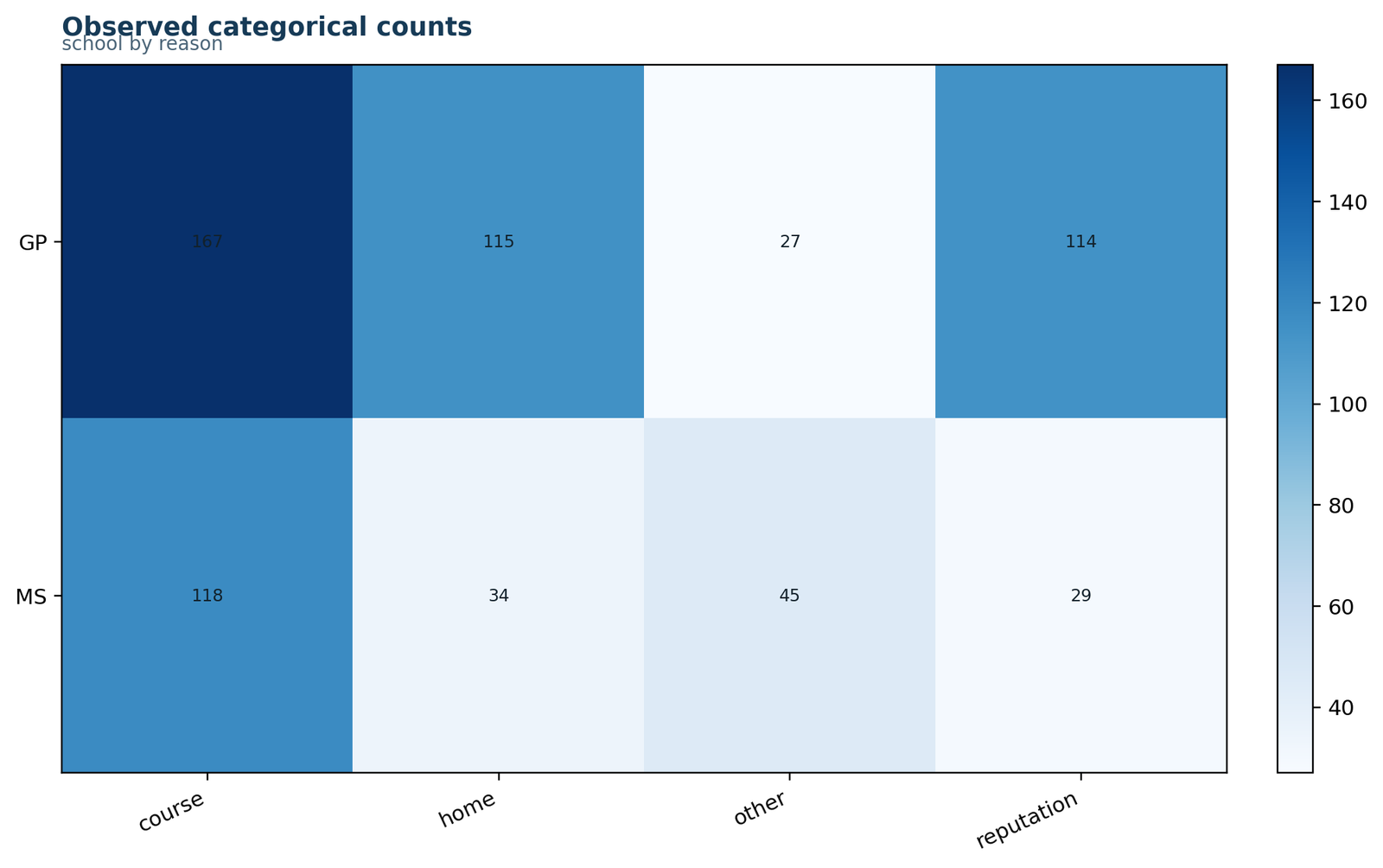
The largest cell is GP–course with 167 observations. GP also has 115 home, 27 other and 114 reputation responses; MS has 118, 34, 45 and 29.
GP total: 423. MS total: 226. Grand total: 649.
Raw counts differ partly because GP has a larger sample. Count comparisons must therefore be standardized through expected counts and within-school percentages.
The heatmap establishes the eight cells from which every expected count, residual and contribution is calculated.
Chart 2: Expected Counts Under HomogeneityPython
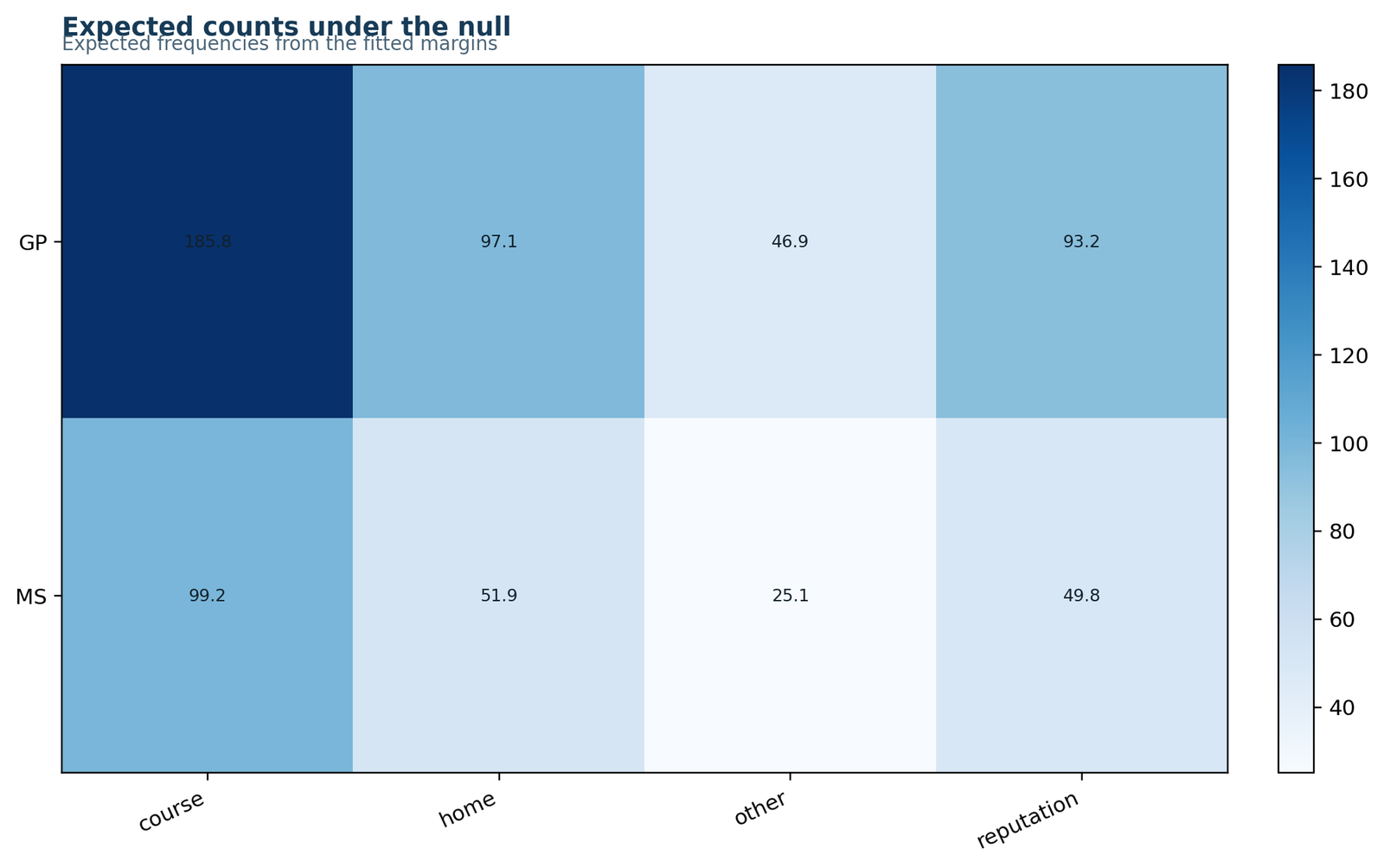
Expected counts preserve the GP and MS sample totals while imposing one common reason distribution. Every expected cell remains well above 5.
GP: 185.755, 97.114, 46.928, 93.203. MS: 99.245, 51.886, 25.072, 49.797.
The expected table is the benchmark for the null hypothesis. Deviations from these values generate the Pearson statistic.
The minimum expected count of 25.072 confirms that sparse-cell concerns do not explain the significant result.
Chart 3: Pearson Residual PatternPython
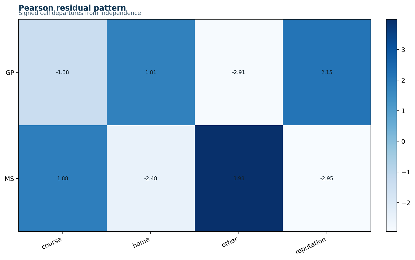
The strongest positive residual is MS–other, while the strongest negative residuals occur for MS–reputation and GP–other.
GP residuals: −1.376, 1.815, −2.909, 2.154. MS residuals: 1.883, −2.483, 3.980, −2.947.
Positive values mean more observations than expected under homogeneity; negative values mean fewer.
Residual signs reveal the direction that the contribution heatmap cannot show because squared contributions are always positive.
Chart 4: Cell Contributions to χ²Python
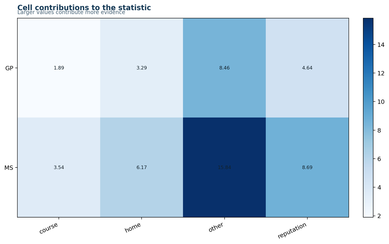
MS–other is the single largest cell contribution, and the paired GP–other cell is also large.
MS–other: 15.8385 or 30.15% of χ². GP–other: 8.4622 or 16.11%. Total: 52.5239.
The “other” category alone contributes 24.3006, nearly half of the global statistic.
Contribution values quantify importance but do not state whether observed counts are above or below expectation.
Chart 5: Within-School Row PercentagesPython
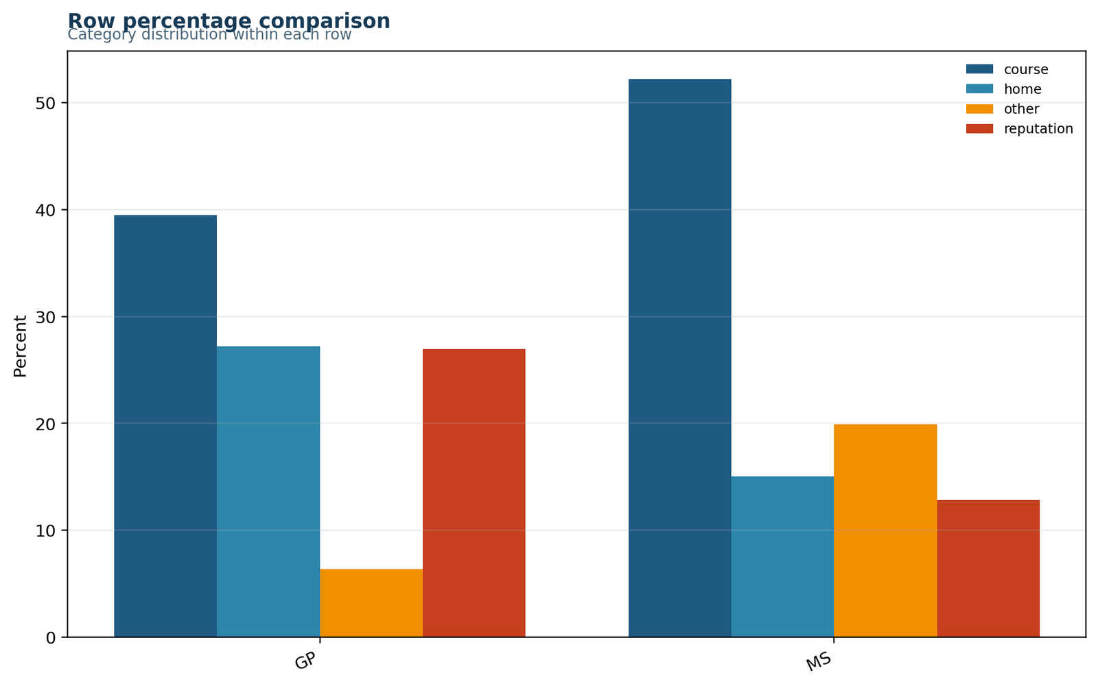
MS has higher percentages for course and other, whereas GP has higher percentages for home and reputation.
GP: 39.48%, 27.19%, 6.38%, 26.95%. MS: 52.21%, 15.04%, 19.91%, 12.83%.
The largest percentage-point contrast is reputation at −14.12 points for MS relative to GP, followed by other at +13.53 points.
Homogeneity is fundamentally a statement about equal percentages, so this chart directly communicates the substantive departure.
Chart 6: Model DiagnosticsPython
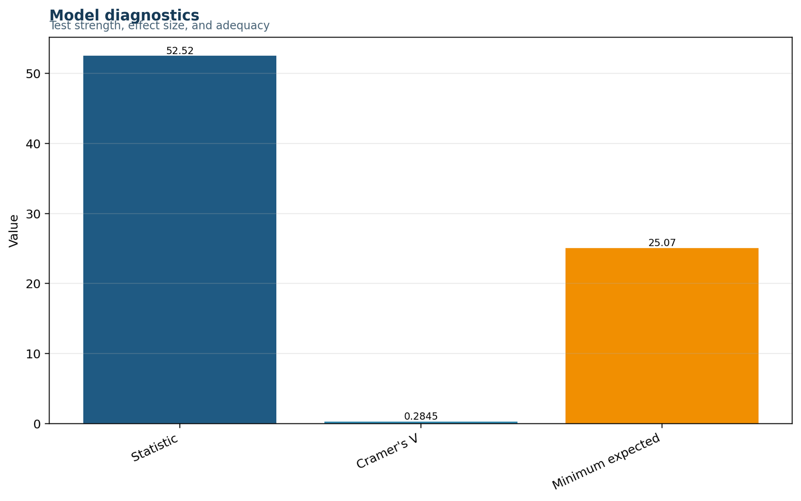
The test statistic is large relative to its three-degree-of-freedom reference distribution, while expected-count adequacy is strong.
χ²: 52.5239. Cramér’s V: 0.2845. Minimum expected: 25.0724.
The chi square test for homogeneity p-value establishes evidence, Cramér’s V describes magnitude and the minimum expected count supports the approximation.
These metrics answer different questions and should not be interpreted on a common numerical scale simply because they appear together.
Chart 7: Population Category ProfilesPython
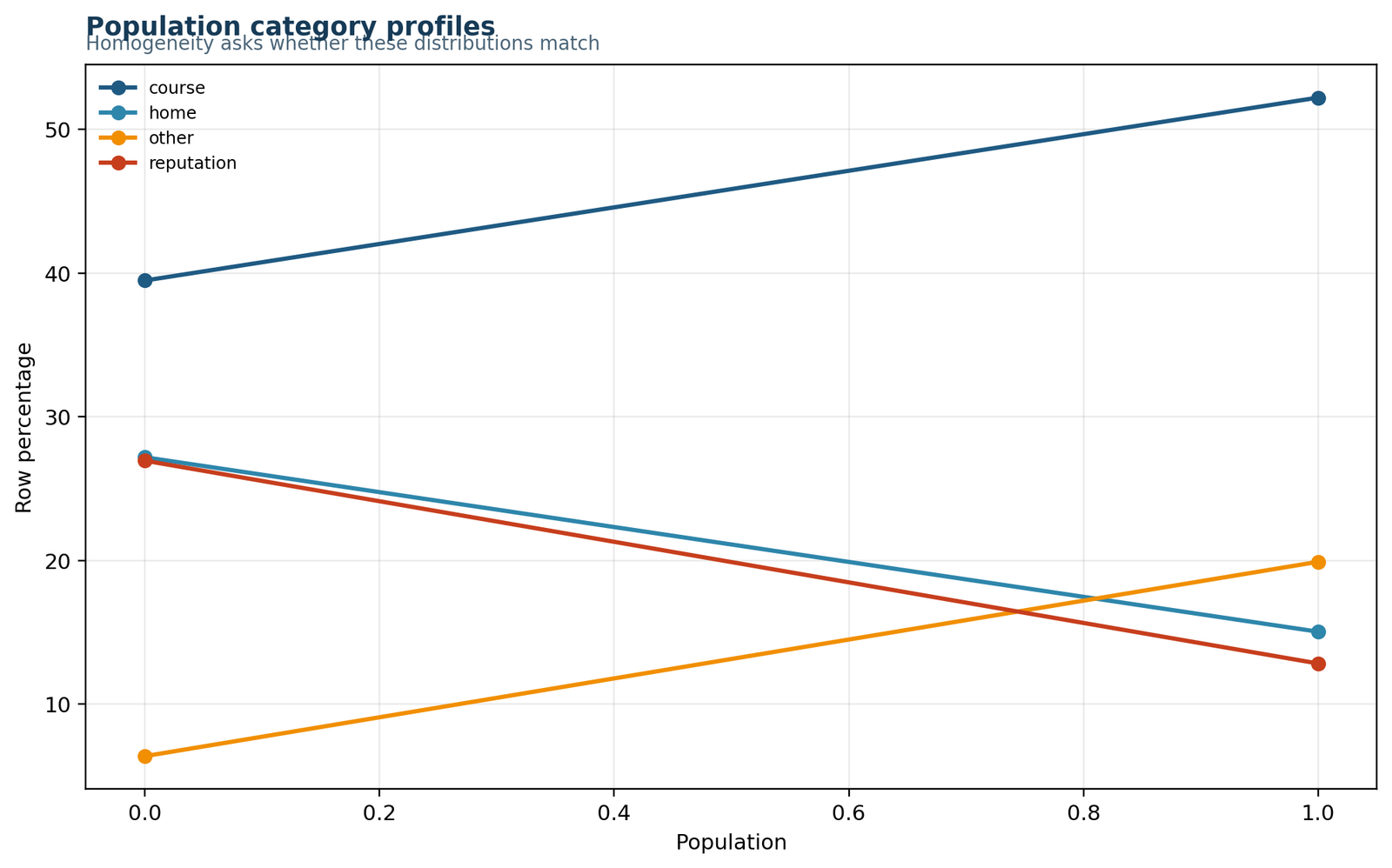
Course rises from 39.48% to 52.21% and other rises from 6.38% to 19.91%; home and reputation fall sharply.
Changes from GP to MS: course +12.73, home −12.14, other +13.53 and reputation −14.12 percentage points.
Parallel or overlapping profiles would support homogeneity. The crossing and separation visible here represent a changed categorical composition.
The profile view makes the omnibus difference understandable without reducing it to one category.
R Chi Square Test for Homogeneity Chart Pairs
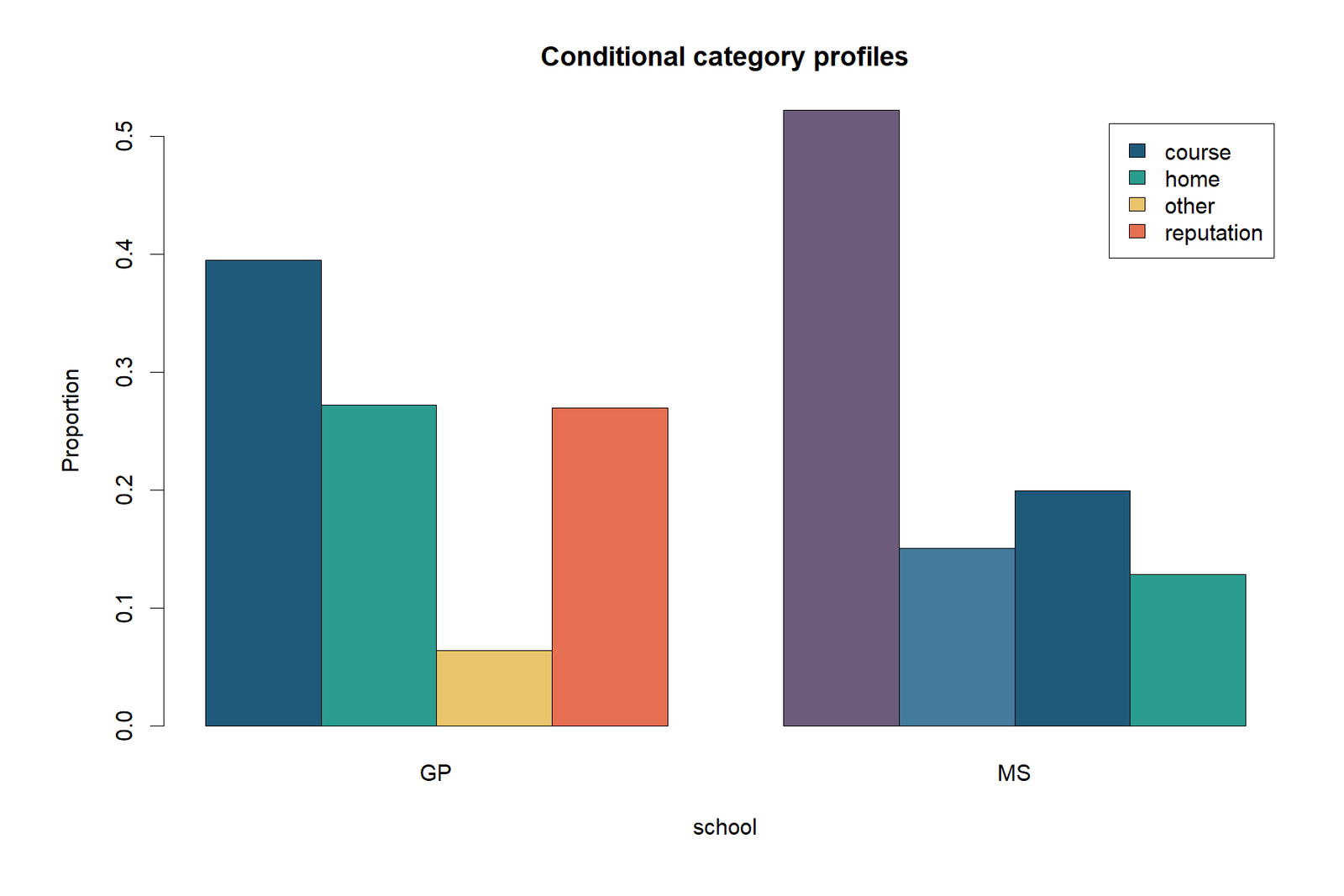
The R report reproduces the observed, expected, residual and contribution information and adds a conditional row-profile chart and a compact result summary. For the chi square test for homogeneity, the first four supplied R image URLs match the corresponding cross-software figures, while the final two are R-specific visual outputs.
Observed Counts
GP contributes 167, 115, 27 and 114 observations; MS contributes 118, 34, 45 and 29. The unequal row totals make raw-count-only interpretation incomplete.
Expected Counts
Under homogeneity, expected GP counts are 185.755, 97.114, 46.928 and 93.203; expected MS counts are 99.245, 51.886, 25.072 and 49.797.
Pearson Residuals
MS–other has residual +3.980, indicating substantially more “other” responses than expected. GP–other is −2.909, showing the complementary deficit.
Cell Contributions
MS–other contributes 15.8385 and GP–other contributes 8.4622. Together they explain 46.27% of χ².
Row Profiles
The GP profile is 0.3948, 0.2719, 0.0638 and 0.2695. The MS profile is 0.5221, 0.1504, 0.1991 and 0.1283. The profiles visibly differ.
Result Summary
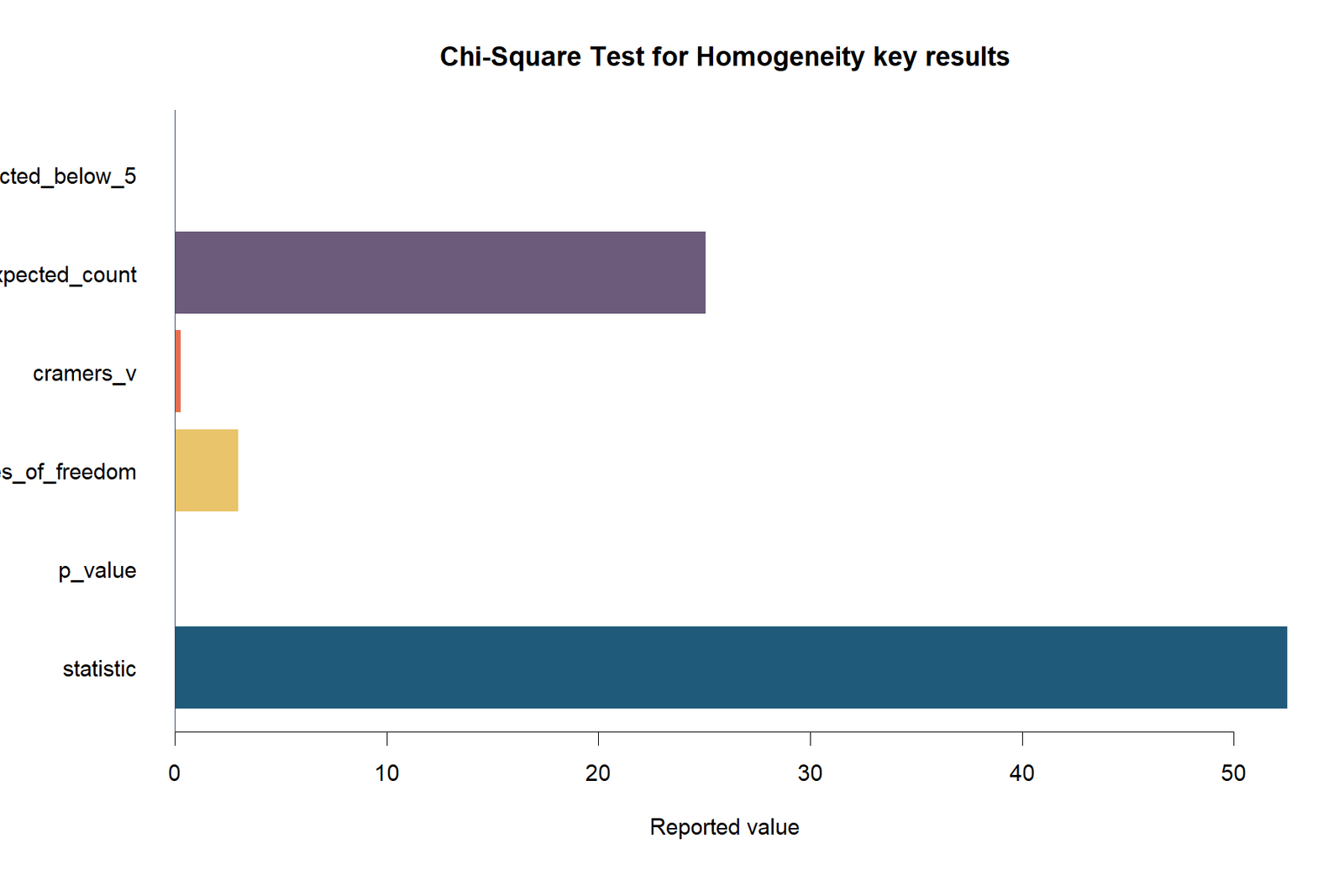
The chi square test for homogeneity summary visual displays χ² = 52.5239, df = 3, Cramér’s V = 0.2845, minimum expected = 25.0724 and zero expected cells below 5.
Chi Square Test for Homogeneity in Python, R, SPSS, Excel and Other Software
Chi Square Test for Homogeneity in Python
Use scipy.stats.chi2_contingency with correction disabled for the ordinary Pearson r × c test. Calculate row percentages, residuals, contributions and Cramér’s V separately.
- Observed matrix shape: 2 × 4
- Continuity correction: not used for this table
- Expected counts returned automatically
- Residuals: (observed − expected)/√expected
- Cramér’s V based on χ², n and minimum dimension
Chi Square Test for Homogeneity in R
Use chisq.test(observed, correct = FALSE). R returns Pearson X-squared, df, p-value, expected counts and Pearson residuals.
- Keep school levels as rows and reasons as columns.
- Use
prop.table(observed, 1)for row profiles. - Square Pearson residuals for cell contributions.
- Calculate Cramér’s V explicitly or with a validated package.
Chi Square Test for Homogeneity in SPSS
SPSS uses CROSSTABS. Request counts, row percentages, expected counts, residuals, standardized residuals, CHISQ and PHI.
- Analyze → Descriptive Statistics → Crosstabs
- Rows: school; Columns: reason
- Statistics: Chi-square, Phi and Cramér’s V
- Cells: observed, expected, row %, residuals
- Report Pearson Chi-Square, not only “Sig. = .000”
Chi Square Test for Homogeneity in Excel
Build an observed table, calculate row and column totals, derive expected counts and use CHISQ.TEST for the p-value. Calculate χ² explicitly by summing cell contributions.
- Expected = row total × column total / grand total
- Contribution = (observed − expected)^2 / expected
- Statistic = sum of contributions
- df = (rows − 1)(columns − 1)
- Cramér’s V = SQRT(statistic/(n×MIN(r−1,c−1)))
Chi Square Test for Homogeneity in Stata
For row-level data, use tabulate school reason, chi2 row expected. Stata reports Pearson chi-square and row percentages. Use additional commands or calculations for Cramér’s V and cell diagnostics.
Chi Square Test for Homogeneity in SAS
Use PROC FREQ with TABLES school*reason / CHISQ EXPECTED DEVIATION CELLCHI2;. Request measures of association when effect size is needed.
Chi Square Test for Homogeneity in Minitab
Use Stat → Tables → Chi-Square Test for Association when observations are summarized, or Cross Tabulation and Chi-Square for row-level data. Interpret the result as homogeneity when samples came from separate populations.
Chi Square Test for Homogeneity in Google Sheets
Use the same observed and expected formulas as Excel. CHISQ.TEST returns the p-value, while the statistic and residual diagnostics should be calculated in supporting cells for transparent reporting.
Cross-Software Agreement
| Output | Python | R | SPSS |
|---|---|---|---|
| Pearson χ² | 52.52394157 | 52.52394157 | 52.524 |
| df | 3 | 3 | 3 |
| P-value | 2.315976089e−11 | 2.315976089e−11 | < .001 |
| Cramér’s V | 0.28448299 | 0.28448299 | 0.284 |
| Minimum expected | 25.07241911 | 25.07241911 | 25.07 |
| Expected below 5 | 0 | 0 | 0 |
Why Rounded SPSS Output Looks Different
SPSS prints the p-value as .000 when it is smaller than .0005 under the displayed precision. The correct report is p < .001, not p = .000. Python and R retain scientific notation and reveal the much smaller underlying value.
Expandable Chi Square Test for Homogeneity Code
Use the expandable panels to copy a transparent implementation. Always verify table orientation, labels and expected counts before interpreting the p-value.
Python code
import numpy as np
from scipy.stats import chi2_contingency

observed = np.array([
    [167, 115, 27, 114],  # GP
    [118,  34, 45,  29],  # MS
])

chi2, p_value, df, expected = chi2_contingency(observed, correction=False)
pearson_residuals = (observed - expected) / np.sqrt(expected)
cell_contributions = (observed - expected) ** 2 / expected
row_percentages = observed / observed.sum(axis=1, keepdims=True) * 100
n = observed.sum()
cramers_v = np.sqrt(chi2 / (n * min(observed.shape[0]-1, observed.shape[1]-1)))

print(chi2, p_value, df)
print(expected)
print(pearson_residuals)
print(cell_contributions)
print(row_percentages)
print(cramers_v)
R code
observed <- matrix(
  c(167, 115, 27, 114,
    118,  34, 45,  29),
  nrow = 2, byrow = TRUE,
  dimnames = list(
    school = c("GP", "MS"),
    reason = c("course", "home", "other", "reputation")
  )
)

fit <- chisq.test(observed, correct = FALSE)
row_profiles <- prop.table(observed, margin = 1)
cell_contributions <- fit$residuals^2
n <- sum(observed)
cramers_v <- sqrt(unname(fit$statistic) /
                  (n * min(nrow(observed)-1, ncol(observed)-1)))

fit$statistic
fit$parameter
fit$p.value
fit$expected
fit$residuals
cell_contributions
row_profiles
cramers_v
SPSS syntax
CROSSTABS
  /TABLES=school_n BY reason_n
  /FORMAT=AVALUE TABLES
  /STATISTICS=CHISQ PHI
  /CELLS=COUNT ROW COLUMN EXPECTED RESID SRESID
  /COUNT ROUND CELL.
Excel formulas
Observed table: B4:E5
Row totals: F4 = SUM(B4:E4), F5 = SUM(B5:E5)
Column totals: B6 = SUM(B4:B5), fill right to E6
Grand total: F6 = SUM(F4:F5)
Expected B10: =$F4*B$6/$F$6
Fill B10:E11
Cell contribution B14: =(B4-B10)^2/B10
Fill B14:E15
Chi-square statistic: =SUM(B14:E15)
Degrees of freedom: =(ROWS(B4:E5)-1)*(COLUMNS(B4:E5)-1)
P-value: =CHISQ.DIST.RT(statistic_cell, df_cell)
Direct p-value check: =CHISQ.TEST(B4:E5,B10:E11)
Cramer's V: =SQRT(statistic_cell/(F6*MIN(ROWS(B4:E5)-1,COLUMNS(B4:E5)-1)))
Expected Code Output
| Quantity | Expected output |
|---|---|
| χ² | 52.52394157003515 |
| df | 3 |
| p | 2.315976089451305e−11 |
| Cramér’s V | 0.2844829916304641 |
| Minimum expected | 25.07241910631741 |
Advanced Chi Square Test for Homogeneity Topics
Effect Size Is Separate from Significance
The chi square test for homogeneity p-value is sensitive to sample size and asks whether the distributions are exactly equal under the null. Cramér’s V measures the strength of association in the observed table. Reporting both prevents a large sample from turning a small discrepancy into an overstated practical claim.
Interpreting Cramér’s V
Rules such as .10 small, .30 medium and .50 large are rough conventions, especially because appropriate benchmarks depend on table dimensions, category prevalence and field context. V = .284 is close to the common medium benchmark and is consistent with the large percentage-point shifts visible in the row profiles.
Adjusted Residual Multiplicity
Eight adjusted residuals are shown, but pairs within each category are algebraically linked in a 2 × c table. For formal follow-up, define a small set of scientifically meaningful contrasts and use Holm, Bonferroni or a model-based simultaneous inference procedure.
Partitioning the Chi-Square Statistic
Categories can sometimes be grouped into planned contrasts, such as course versus non-course or institution-related reasons versus personal reasons. Partitions should be prespecified and statistically independent when separate components are interpreted. Data-driven regrouping can inflate false-positive findings and obscure the original construct.
Structural Zeros
A structural zero is a cell that cannot occur by design. It must not be treated as an ordinary sampling zero. Structural zeros change the model, degrees of freedom and expected-count calculation. The worked table has no structural zeros because every reason category is possible at both schools.
Survey Weights and Complex Samples
If students were selected through stratified or clustered sampling, ordinary Pearson inference may underestimate uncertainty. Survey-adjusted Rao–Scott chi-square tests account for design weights, strata and clusters. Raw weighted counts should not simply be inserted into the ordinary formula without design correction.
Power and Sample Size
Power depends on the total sample size, table dimensions, allocation across populations and the true difference in category profiles. Prospective planning can use Cohen’s w or a specified set of population proportions. A power calculation should reflect the exact r × c design rather than relying on generic “30 per group” rules.
Confidence Intervals for Category Differences
The global chi square test for homogeneity does not produce confidence intervals for individual percentage differences. Analysts can report confidence intervals for prespecified differences in proportions, with multiplicity adjustment when several categories are examined. Simultaneous multinomial confidence regions provide a more comprehensive but more advanced alternative.
Log-Linear Interpretation
The homogeneity null is equivalent to a log-linear model without a school × reason interaction. Rejecting the null indicates that the interaction is needed to reproduce the observed table. This connection becomes useful for multiway tables and hierarchical model comparisons.
Multinomial Regression Interpretation
With reason as a four-category outcome and school as a predictor, multinomial logistic regression tests whether the vector of school coefficients is zero. It also produces category-specific relative risk ratios and can adjust for additional variables. The unadjusted likelihood-ratio test is closely related to the contingency-table analysis.
Sensitivity to Category Definition
Combining or splitting categories changes df, expected counts and effect size. Categories should be defined substantively before analysis. In this dataset, “other” is highly influential; merging it after seeing the result would erase an important pattern and constitute outcome-driven recoding.
Large-Sample Versus Exact Inference
The minimum expected count is 25.07, so asymptotic inference is reliable. Exact or Monte Carlo methods would be computationally possible but unnecessary for resolving sparse-cell uncertainty. They would not change the substantive importance of the row-profile differences.
APA Reporting for a Chi Square Test for Homogeneity
An APA-style report should identify the variables and populations, present the test statistic with degrees of freedom and sample size, report the p-value correctly, include Cramér’s V, and summarize the most important category-profile differences.
Concise APA Result
A chi-square test for homogeneity indicated that the distribution of school-choice reasons differed between GP and MS students, χ²(3, N = 649) = 52.52, p < .001, Cramér’s V = .284.
Expanded APA Result
The school-choice reason distribution differed significantly across the GP and MS school populations, χ²(3, N = 649) = 52.52, p < .001, Cramér’s V = .284. Compared with GP, MS had higher percentages selecting course (52.21% vs. 39.48%) and other (19.91% vs. 6.38%), and lower percentages selecting home (15.04% vs. 27.19%) and reputation (12.83% vs. 26.95%).
APA Method Sentence
A Pearson chi-square test for homogeneity was conducted to compare the distribution of the categorical school-choice reason variable across independently sampled GP and MS student populations.
APA Assumption Sentence
Expected-frequency conditions were satisfied; no expected cell count was below 5, and the minimum expected count was 25.07.
APA Follow-Up Sentence
Cell diagnostics indicated that the “other” category contributed most strongly to the global result, with fewer GP students and more MS students than expected under a common reason distribution.
Fill-in Reporting Templates
Significant Result
Reject H₀
A chi-square test for homogeneity showed that the distribution of response variable differed across populations.
χ²(df, N = N) = statistic, p < threshold, Cramér’s V = effect size.
Nonsignificant Result
Fail to reject H₀
A chi-square test for homogeneity did not provide sufficient evidence that the distribution of response variable differed across populations.
χ²(df, N = N) = statistic, p = p-value, Cramér’s V = effect size.
What Not to Write
- Do not write p = .000; use p < .001.
- Do not say “accept the alternative with 100% confidence.”
- Do not claim every category differs merely because the global test is significant.
- Do not omit population percentages and report only the p-value.
- Do not describe the result as causal unless treatment assignment and design support causality.
Common Chi Square Test for Homogeneity Mistakes
Mistakes in Setup
- Entering percentages instead of counts.
- Mixing category order between populations.
- Counting one person more than once.
- Using the test with paired or repeated responses.
- Choosing homogeneity when there is only one sample and fixed expected probabilities.
- Combining categories only because the first test was inconvenient.
Mistakes in Interpretation
- Saying p < .05 proves the distributions are homogeneous.
- Reporting p = .000 from rounded SPSS output.
- Ignoring Cramér’s V and practical magnitude.
- Using raw counts to compare groups of different sizes.
- Reading cell contributions as signed differences.
- Claiming causation from an observational comparison.
Confusing Homogeneity and Independence
Chi square test for homogeneity and independence calculations are identical, so software may not distinguish them. The cure is to write the sampling design before opening the software. Separate population samples imply a homogeneity question; one sample with two measured categorical variables implies independence.
Using “Two-Tailed” Language
The chi-square reference probability is taken from the upper tail because large discrepancies reject the null. The substantive alternative allows any direction of distributional difference. Say “right-tail chi-square test with a nondirectional alternative,” or simply report the standard chi-square test.
Stopping at the Global P-Value
A chi square test for homogeneity p-value does not tell readers that MS has more course and other responses while GP has more home and reputation responses. Include row percentages and residual diagnostics.
Ignoring Sampling Fractions and Clusters
Students within the same classroom or household may be correlated. A simple table cannot diagnose this. Design-based or multilevel methods may be necessary even when expected counts are large.
Overinterpreting Residual Thresholds
Using |residual| > 1.96 for every cell without multiplicity correction can overstate follow-up evidence. Treat residuals as diagnostic unless a planned inferential procedure is reported.
Chi Square Test for Homogeneity Practice Problems
Practice Problem 1: Test Selection
Independent random samples of adults are taken from four regions. Each person selects one of five preferred news sources. Which test is appropriate?
Answer and reasoning
Use a chi square test for homogeneity because separate regional populations are sampled and the distribution of one five-category response is compared across them.
Practice Problem 2: Hypotheses
Write hypotheses for comparing transport-mode distributions across urban, suburban and rural populations.
Answer and reasoning
H0: the distribution of transport mode is the same in all three populations. HA: at least one population has a different transport-mode distribution.
Practice Problem 3: Expected Count
A row total is 180, a category column total is 75 and the grand total is 500. Find the expected count.
Answer and reasoning
E = 180 × 75 / 500 = 27.
Practice Problem 4: Degrees of Freedom
Four populations are compared across six response categories. Find df.
Answer and reasoning
df = (4 − 1)(6 − 1) = 15.
Practice Problem 5: Residual Sign
An observed count is 42 and its expected count is 30. Is the Pearson residual positive or negative?
Answer and reasoning
Positive, because observed exceeds expected. The residual is (42 − 30)/√30 ≈ 2.191.
Practice Problem 6: Assumption Check
A 3 × 4 table has two expected counts below 5 and one expected count below 1. Is the usual approximation acceptable?
Answer and reasoning
No. For a chi square test for homogeneity, the count below 1 violates common guidance, and 2 of 12 cells below 5 require careful evaluation. Consider justified category combination, exact or Monte Carlo inference, or a suitable model.
Practice Problem 7: Interpretation
A test gives χ²(6) = 14.8, p = .022, V = .12. Write a conclusion.
Answer and reasoning
Reject the equal-distribution null at α = .05. The distributions differ, but V = .12 suggests a relatively small association. Describe population percentages and follow-up cells.
Practice Problem 8: Homogeneity or Independence?
One random sample of 900 voters is classified by education level and candidate preference.
Answer and reasoning
This is naturally a chi square test of independence because two categorical variables are measured in one sample from one population.
Practice Problem 9: Worked Table Check
Which worked cell contributes most to χ²?
Answer and reasoning
MS–other contributes 15.8385, the largest of the eight cells and 30.15% of the total statistic.
Practice Problem 10: APA Reporting
Write the worked result in one sentence.
Answer and reasoning
The distribution of school-choice reasons differed between GP and MS students, χ²(3, N = 649) = 52.52, p < .001, Cramér’s V = .284.
Chi Square Test for Homogeneity AP Statistics Study Notes
AP Statistics Four-Step Structure
- State: identify the populations, categorical response and hypotheses.
- Plan: name a chi square test for homogeneity and check randomization, independence and expected counts.
- Do: calculate expected counts, χ², df and p-value.
- Conclude: make a contextual population statement using the p-value and significance level.
AP Statistics Keywords
| Wording clue | Likely procedure |
|---|---|
| Separate random samples from several populations; compare a response distribution | Chi square test for homogeneity |
| One sample; two categorical variables measured on each person | Chi square test of independence |
| One sample; compare one categorical variable with claimed probabilities | Chi square goodness-of-fit test |
Conditions to Write on an Exam
- Random: samples or assignment were random, or the prompt provides a defensible randomization statement.
- Independent: observations are independent; when sampling without replacement, each sample is less than 10% of its population.
- Large counts: all expected counts are at least 5 under the standard AP condition.
Calculator Evidence to Show
Even when a calculator provides the result, show the hypotheses, expected-count condition, df and contextual conclusion. A screen value without a plan or conclusion does not demonstrate statistical reasoning.
Fast Memory Rule
Homogeneity = same response, different populations. Independence = two variables, one population. Goodness of fit = one variable, one claimed distribution.
Worked AP-Style Conclusion
Because p = 2.316 × 10⁻¹¹ is less than α = .05, reject H0. There is convincing evidence that the distribution of school-choice reasons is not the same for GP and MS students.
Chi Square Test for Homogeneity Downloads
Use the reports to verify software output and the worked spreadsheet to reproduce observed counts, expected counts, contributions, residuals and summary measures.
R PDF ReportVerified R output with the test result and chart sequence.
SPSS PDF OutputCrosstabs, expected counts, standardized residuals, chi-square table, Cramér’s V and chart.
Worked Excel AnalysisFormula-based workbook for the complete chi square test for homogeneity calculation.
Values to Verify After Download
| Item | Verified value |
|---|---|
| Valid rows | 649 |
| Observed table | [[167, 115, 27, 114], [118, 34, 45, 29]] |
| Pearson χ² | 52.52394157003515 |
| df | 3 |
| p-value | 2.315976089451305e−11 |
| Cramér’s V | 0.2844829916304641 |
| Minimum expected | 25.07241910631741 |
| Expected below 5 | 0 |
Frequently Asked Questions
What is a chi square test for homogeneity?
A chi square test for homogeneity compares the distribution of one categorical response across two or more independent populations or groups.
When do you use a chi square test for homogeneity?
Use a chi square test for homogeneity when separate samples or randomized groups are compared using the same categorical response categories and expected counts are adequate.
What is the null hypothesis?
In a chi square test for homogeneity, the response-category proportions are the same in all populations; equivalently, the response distribution is homogeneous across populations.
What is the alternative hypothesis?
For a chi square test for homogeneity, at least one population has a different response distribution. The chi square test for homogeneity alternative does not specify which category differs.
How is the expected count calculated?
In a chi square test for homogeneity, multiply the cell’s row total by its column total and divide by the grand total.
What are the degrees of freedom?
For a chi square test for homogeneity with an r × c table, df = (r − 1)(c − 1). The worked 2 × 4 table has df = 3.
Is a chi square test for homogeneity one-tailed or two-tailed?
A chi square test for homogeneity uses a reference probability in the right tail of the chi-square distribution because only large discrepancies reject the null. The substantive alternative is nondirectional.
What is the difference between homogeneity and independence?
A chi square test for homogeneity compares one response distribution across separately sampled populations. Independence examines association between two categorical variables in one sampled population. The table calculation is the same.
What is the difference between homogeneity and goodness of fit?
A chi square test for homogeneity compares populations using pooled estimated category proportions. Goodness of fit compares one sample with probabilities specified in advance.
What assumptions are required?
A chi square test for homogeneity requires categorical counts, mutually exclusive categories, independent observations, independent samples or groups, comparable response coding, adequate expected counts and a defensible sampling or assignment design.
What if expected counts are below 5?
For a chi square test for homogeneity, consider justified category consolidation, exact or Monte Carlo inference, or a model suited to sparse categorical data. Do not ignore the problem.
How do you interpret a significant result?
For a significant chi square test for homogeneity, conclude that the response distributions are not the same across populations, then inspect percentages, residuals and contributions to describe the pattern.
How do you interpret a nonsignificant result?
State that the data do not provide sufficient evidence of different population distributions. Do not claim the distributions are proven identical.
What is Cramér’s V?
It is an effect-size measure for contingency tables. In the worked example V = 0.2845, indicating a meaningful association.
What cell drives the worked result?
MS–other has the largest contribution, 15.8385, while both “other” cells jointly account for 46.27% of χ².
Can the test prove causation?
Not from observational samples alone. Random assignment and an appropriate experimental design are required for a causal treatment conclusion.
Can I use percentages in the calculator?
Enter counts. Percentages can be interpreted afterward but must not replace frequencies without their denominators.
How do I report SPSS p = .000?
Report p < .001. A p-value is not exactly zero; SPSS has rounded it.
Can the test have more than two populations?
Yes. The method handles any r × c table when assumptions are satisfied.
What result should the worked data produce?
χ²(3) = 52.52394157, p = 2.315976089 × 10⁻¹¹, Cramér’s V = 0.28448299 and minimum expected count = 25.0724.
Conclusion
The chi square test for homogeneity is the correct global procedure when independent population samples or treatment groups are compared on the distribution of one categorical response. Its calculation uses the same Pearson contingency-table formula as a test of independence, but the sampling design changes the inferential statement.
In the verified school example, the reason distributions differ strongly between GP and MS, χ²(3, N = 649) = 52.52, p < .001, Cramér’s V = .284. All expected counts are adequate. MS has higher course and other percentages, while GP has higher home and reputation percentages. The “other” category contributes the largest share of the global discrepancy.
A complete analysis therefore includes more than a calculator p-value. It states the population design, hypotheses and assumptions; reports observed and expected counts; interprets row percentages, residuals and contributions; gives Cramér’s V; and uses correct contextual wording in Python, R, SPSS, Excel or another validated workflow.

