
Regression Residual Analysis: Formulas, Diagnostic Plots, Thresholds and Interpretation
Regression Residual Analysis examines the errors left after a regression model is fitted. This complete worked guide evaluates a five-predictor model for final grade G3 using residual plots, normality checks, heteroscedasticity tests, specification testing, leverage, Cook’s distance, DFFITS, COVRATIO and documented case review in Python, R, SPSS and Excel.
Regression Residual Analysis Model Overview
Regression Residual Analysis is the systematic study of observed-minus-predicted errors after a regression equation has been estimated. The purpose is not merely to calculate a residual column. The purpose is to determine whether the fitted mean structure is credible, whether uncertainty is being estimated under reasonable conditions, whether a small number of observations has disproportionate influence, and whether the final scientific or practical conclusion remains stable when legitimate diagnostic concerns are addressed.
The worked research question is: Does the linear model that predicts final grade G3 from G1, G2, studytime, failures and absences provide an adequate and stable representation of the 649 complete observations? The fitted equation has strong average explanatory power, with R² = 0.850563 and adjusted R² = 0.849401. However, Regression Residual Analysis asks a different question from model fit alone. It examines what the model fails to explain, how those failures are distributed, and whether the reported slopes and intervals are sensitive to functional form, nonconstant variance or influential cases.
What Is Regression Residual Analysis?
For observation i, the raw residual is the observed outcome minus the fitted outcome. A positive residual means the model underpredicted G3; a negative residual means the model overpredicted G3. Residuals are expressed in outcome units, so a raw residual of 2 means the recorded final grade was two points above the fitted value. Standardized and studentized residuals place that error on a scale that accounts for residual spread and, in different ways, leverage.
The fitted value comes from the declared five-predictor equation. Every residual, leverage value and influence statistic in this article is model-specific. Adding a predictor, changing a transformation, removing the intercept or changing the eligible rows changes the fitted values and therefore changes the entire Regression Residual Analysis.
What Question Does Regression Residual Analysis Answer?
Regression Residual Analysis answers whether the residual behavior is compatible with the claims attached to the fitted regression. It evaluates linearity of the conditional mean, constancy of residual variance, approximate distributional behavior for conventional inference, dependence at the relevant observation order, and case influence. It also separates four ideas that are often confused: a response outlier can have a large residual, a high-leverage observation can have an unusual predictor combination, an influential observation can materially change estimates, and an erroneous observation is one contradicted by the source record. These categories overlap, but they are not interchangeable.
When Should Regression Residual Analysis Be Used?
Use it when
- A linear or generalized regression model will be interpreted, reported or used for prediction.
- R², coefficients or p-values look persuasive but the adequacy of the fitted equation has not been checked.
- The outcome may contain unusual values, boundaries, floor effects or ceiling effects.
- Predictor combinations may create high leverage or case influence.
- Conventional standard errors and confidence intervals depend on variance or distribution assumptions.
- A transparent case-review and sensitivity record is required for publication or professional work.
Do not use it as
- An automatic deletion system for every observation beyond a threshold.
- A substitute for choosing the correct regression family and link function.
- Proof of causality, measurement validity or correct data collection.
- A guarantee of independence when the sampling design contains clusters or repeated measurements.
- A reason to transform variables until every plot appears visually perfect.
- A collection of disconnected tests without a documented decision rule.
Why Use It Instead of R² Alone?
R² summarizes the proportion of sample variation in G3 represented by the fitted values. It does not test whether residual variance is constant, whether the functional form is adequate, whether tails are approximately normal, or whether a few observations dominate the coefficients. In this example, R² is approximately 0.85, yet the Ramsey RESET test, Breusch–Pagan test, White test, Shapiro–Wilk test and Jarque–Bera test all identify important conflicts. The model therefore has a useful conditional mean while still requiring cautious inference and specification review.
How the Diagnostic Quantities Work
Here, p is the number of fitted coefficients including the intercept, so p = 6. The article uses transparent screening lines rather than universal pass/fail laws: leverage above 2p/n, Cook’s distance above 4/n, absolute DFFITS above 2√(p/n), externally studentized residual magnitude above 3, and COVRATIO outside 1 ± 3p/n. These thresholds prioritize cases for review; they do not establish invalidity.
How Residuals, Coefficients and Predictions Are Interpreted
A residual describes one observation’s signed error under the fitted equation. A coefficient describes the expected change in fitted G3 associated with a one-unit predictor increase while the other included predictors are held constant. A predicted value is the conditional mean generated by the equation for a specified predictor profile. Influence statistics describe how much the estimated model would change if an observation were omitted. Regression Residual Analysis keeps these scales separate so that a large residual is not mistakenly interpreted as a large coefficient and a high-leverage point is not automatically labeled an outcome outlier.
How Regression Residual Analysis Differs from Related Methods
Regression Residual Analysis is broader than a normality test because it also evaluates form, variance, dependence and influence. It is broader than an outlier check because it distinguishes unusual outcomes from unusual predictor profiles. It differs from robust regression, which changes the estimation rule, and from heteroscedasticity-consistent standard errors, which change the estimated covariance matrix without changing fitted values. It also differs from cross-validation, which evaluates performance on held-out observations. A defensible workflow may use all of these tools, but each answers a different question.
Supported Variables and Model Types
The core logic of Regression Residual Analysis applies to continuous-outcome linear regression and extends, with model-specific residual definitions, to logistic, Poisson, negative binomial, ordinal, survival and multilevel models. The present worked example is ordinary least squares with one continuous outcome and five numeric or ordered predictors. Raw, standardized and studentized residuals are therefore interpreted on the linear-model scale. Deviance and Pearson residuals would be more appropriate for many generalized linear models.
Assumptions and Requirements
Correct outcome and regression family
The equation should match the scale and support of G3. A bounded grade outcome can still be analyzed by OLS for a conditional-mean question, but boundary compression and nonlinearity must be examined rather than ignored.
Fixed model specification during diagnosis
The formula, intercept convention, coding, complete-case rule and row order must remain fixed while residual and influence quantities are compared across software.
Independent observational units
Durbin–Watson cannot replace design knowledge. Repeated students, classroom clusters or temporal ordering require models that represent those dependencies.
Adequate mean structure
Residuals should not retain systematic curvature after the chosen predictors and transformations are included. The significant RESET result makes this requirement a central issue in the worked analysis.
Variance appropriate for the intended inference
Constant variance is required for conventional homoscedastic OLS standard errors. Point estimates remain OLS estimates under heteroscedasticity, but conventional uncertainty can be misleading.
Documented case-review rules
Thresholds must be defined before selective deletion. Valid unusual observations should normally remain in the primary analysis, with sensitivity results reported separately.
Advantages and Limitations
Advantages
- Connects visual patterns to exact tests and case-level values.
- Separates outlier, leverage, influence and data-error concepts.
- Supports transparent sensitivity analysis instead of hidden cleaning.
- Improves reporting of model limitations and uncertainty.
- Can be reproduced across Python, R, SPSS and Excel.
Limitations
- No diagnostic proves that a model is correct.
- Large samples can make small departures statistically significant.
- Thresholds are screening conventions, not scientific constants.
- Plots require judgment and can be affected by scale or overplotting.
- Remedies such as transformations or deletion can create new interpretation problems.
Model-Review and Remedy Logic
The correct sequence is to fit the prespecified equation, verify coding and rows, inspect broad residual patterns, run formal checks, review case-level influence, identify the likely mechanism, and then compare a scientifically justified alternative. Nonlinearity may call for transformations, interactions, polynomial terms or splines. Heteroscedasticity may call for HC3 uncertainty, weighted least squares or an explicit variance model. Clustering may call for multilevel or cluster-robust methods. Influence may call for source verification and sensitivity analysis. The remedy must target the diagnosed mechanism rather than simply make one plot look cleaner.
Current Worked Scenario
The worked Regression Residual Analysis uses 649 complete observations and the formula G3 ~ G1 + G2 + studytime + failures + absences. The model has R² = 0.850563, adjusted R² = 0.849401, RMSE = 1.253722 and F(5, 643) = 731.965860, p = 1.326 × 10−262. Residual independence is not strongly contradicted by Durbin–Watson = 1.857347 for the retained order. However, RESET F = 9.868464, p = 0.001759 indicates possible functional-form error; Breusch–Pagan = 30.129021, p = 1.391 × 10⁻⁵ and White = 66.454172, p = 6.832 × 10⁻⁷ indicate nonconstant variance; and the normality checks identify strong tail departure.
Quick Answer
What the fitted model supports
The five predictors provide a strong description of the conditional mean of G3 in the fitted sample.
- N = 649 complete observations
- R² = 0.850563
- Adjusted R² = 0.849401
- F(5, 643) = 731.965860
- Overall p = 1.326 × 10−262
- RMSE = 1.253722 grade points
What Regression Residual Analysis changes
The diagnostic evidence limits how confidently conventional intervals and tail predictions should be interpreted.
- RESET p = 0.001759
- Breusch–Pagan p = 1.391 × 10⁻⁵
- White p = 6.832 × 10⁻⁷
- 10 externally studentized residual outliers
- 29 Cook’s-distance flags
- 66 distinct cases with at least one screening flag
Table of Contents
- Why this analysis needs Regression Residual Analysis
- How Regression Residual Analysis works
- Variables, coding and data dictionary
- Verified Regression Residual Analysis results
- Ten Python chart stories
- R charts and paired explanations
- Coefficient interpretation
- Predictions and worked residual calculations
- Assumptions and diagnostic decisions
- Python, R, SPSS and Excel workflows
- Expandable software code
- 26 advanced Regression Residual Analysis topics
- APA-style reporting
- Publication checklist
- Downloads and chart resources
- Related Salar Cafe guides
- 16 frequently asked questions
- Regression Residual Analysis conclusion
Why This Analysis Needs Regression Residual Analysis
The five-predictor model is statistically strong enough that a reader could be tempted to stop after the coefficient table. That would miss the central finding of Regression Residual Analysis: the fitted conditional mean is useful, but the remaining errors are not behaving like an uncomplicated homoscedastic Gaussian linear model. Strong negative tail observations affect normality, changing spread affects conventional precision, and possible curvature affects the meaning of a single straight-line slope over the fitted range.
The diagnostic workflow is especially necessary because 66 observations meet at least one screening rule, while the individual flag totals sum to far more than 66. The overlap reveals why counts must be kept at case level. One observation may have high leverage, cross the DFFITS threshold and alter COVRATIO without having an externally studentized residual beyond ±3. Another observation may be a severe response outlier with ordinary leverage. Regression Residual Analysis prevents those cases from being treated as if they represented one problem.
Questions answered here
- Are residuals centered without a systematic curve?
- Does residual spread remain reasonably stable?
- Are tail departures important for conventional inference?
- Which cases have unusual predictor profiles?
- Which cases materially change fitted results?
- What remedy targets the observed diagnostic mechanism?
Questions not answered here
- Whether the predictors cause changes in G3.
- Whether a flagged record is incorrect without source evidence.
- Whether omitted variables are absent from the data-generating process.
- Whether the model will generalize without held-out validation.
- Whether row order represents time, classroom or another dependence structure.
- Whether a transformed model is substantively preferable before interpretation is considered.
How Regression Residual Analysis Works
Confirm the outcome, predictors, coding, intercept, complete-case rule and observation order before calculating diagnostics.
Obtain fitted values, residual scales, leverage, Cook’s distance, DFFITS, COVRATIO and formal specification tests.
Link plots to exact values, inspect source records, choose a mechanism-specific remedy and document sensitivity results.
1. Fit the Declared Equation
The fitted equation produces one predicted G3 value for every complete row. The intercept and five slopes are estimated simultaneously. The resulting residual vector is orthogonal to each included predictor in the ordinary least-squares sample, but that algebraic property does not guarantee normality, constant variance or a correct functional form.
2. Preserve the Residual Sign
Positive values mean underprediction and negative values mean overprediction. The sign is essential. Taking absolute values is useful for magnitude displays such as scale-location plots, but it removes direction and therefore cannot replace the signed residual-versus-fitted graph.
3. Place Errors on Comparable Scales
The deleted estimate s(i) excludes the focal observation when estimating residual spread. This makes the externally studentized residual especially useful for screening severe response outliers. In the worked Regression Residual Analysis, ten cases exceed |tᵢ| > 3 and the maximum absolute value is 7.581732.
4. Measure Leverage and Influence
| Quantity | Primary question | Worked review rule | Flagged cases |
|---|---|---|---|
| Leverage hᵢᵢ | Is the predictor profile unusual? | hᵢᵢ > 2p/n = 0.01848998 | 47 |
| Cook’s distance | Does deletion change the fitted coefficient vector materially? | Dᵢ > 4/n = 0.00616333 | 29 |
| |DFFITS| | Does deletion change the focal fitted value? | |DFFITS| > 2√(p/n) = 0.19230177 | 29 |
| COVRATIO | Does deletion change joint coefficient precision? | Outside 0.97226502 to 1.02773498 | 49 |
| |Externally studentized residual| | Is the observed outcome unusually far from its fitted value? | |tᵢ| > 3 | 10 |
5. Test Model Form and Variance
The Ramsey RESET test adds functions of the fitted values to determine whether the original linear predictor may omit nonlinear structure. The Breusch–Pagan and White tests examine whether residual variance is associated with the fitted design. These tests do not reveal the scientifically correct alternative, so their results must be combined with plots and theory.
6. Consolidate Flags at Case Level
Each threshold creates a Boolean flag. The union across flags contains 66 unique observations. Adding 10 + 47 + 29 + 29 + 49 would be incorrect because many rows cross more than one rule. A case-level matrix should retain the original row identifier, observed outcome, fitted value, raw residual, studentized residual, leverage, influence measures and the specific rules crossed.
7. Select a Mechanism-Specific Response
For the present Regression Residual Analysis, the strongest broad responses are to calculate heteroscedasticity-consistent uncertainty, investigate nonlinear terms supported by subject knowledge, retain valid unusual observations in the primary model, and report a limited sensitivity analysis for the most influential verified cases. Deleting every flagged row would change the target population and could produce an artificially tidy model.
Variables Used, Coding and Data Dictionary
The worked Regression Residual Analysis keeps the same 649 complete rows, variable meanings and coding rules in every software workflow. G3 is the continuous outcome. G1, G2, studytime, failures and absences are entered as additive predictors with an intercept.
| Variable | Model role | Meaning | Coding and interpretation |
|---|---|---|---|
| G3 | Outcome | Final course grade | Continuous observed outcome used to calculate fitted errors; residual = observed G3 − fitted G3. |
| G1 | Predictor | First-period grade | Numeric grade. Its slope is the adjusted expected difference in G3 for a one-point increase. |
| G2 | Predictor | Second-period grade | Numeric grade. It is the dominant adjusted predictor in the fitted equation. |
| studytime | Predictor | Ordered weekly study-time category | Entered as a one-unit numeric step. The coefficient assumes equal linear spacing between category codes. |
| failures | Predictor | Number of prior class failures | Count predictor. A one-unit increase is associated with a lower fitted G3 after adjustment. |
| absences | Predictor | School absence count | Count predictor. The positive adjusted slope is small and should not be interpreted causally. |
Regression Residual Analysis Results
Complete cases used throughout
Six fitted coefficients including intercept
Strong fitted-sample mean representation
R² adjusted for model size
Error magnitude in G3 grade units
Unique observations, not summed flags
Verified Model Fit
| Result | Exact value | Interpretation |
|---|---|---|
| Model formula | G3 ~ G1 + G2 + studytime + failures + absences | All diagnostic quantities refer to this exact additive OLS equation. |
| N | 649 | Complete observations retained in the analysis. |
| R² | 0.8505634419896496 | Approximately 85.06% of fitted-sample G3 variation is represented by the model. |
| Adjusted R² | 0.8494014158775940 | Fit adjusted for the five predictors. |
| F statistic | 731.9658596010541 | The predictor set is jointly associated with G3. |
| Overall model p | 1.3257355956912994 × 10−262 | The null that all five slopes equal zero is rejected. |
| RMSE | 1.2537218471492084 | Typical squared-error scale is about 1.25 grade points. |
Formal Diagnostic Tests
| Diagnostic | Statistic | p-value | Worked interpretation |
|---|---|---|---|
| Ramsey RESET | F = 9.868463808854484 | 0.0017586743578903211 | Potential omitted nonlinear structure or functional-form error. |
| Breusch–Pagan | 30.129020777320218 | 1.391073405033745 × 10⁻⁵ | Residual variance is not adequately described as constant. |
| White test | 66.45417175310052 | 6.831804065114402 × 10⁻⁷ | A broader heteroscedasticity check also rejects constant variance. |
| Shapiro–Wilk | W = 0.7565722065534948 | 7.721862065650793 × 10⁻³⁰ | Residual distribution differs strongly from a normal reference. |
| Jarque–Bera | 10019.316609810166 | Reported as 0 by numerical output | Skewness and/or kurtosis departure is extreme; the value should be described as below machine display precision, not literally impossible. |
| Durbin–Watson | 1.857347495275311 | Not a conventional p-value test here | Near two for the retained order, but design-based independence still requires substantive verification. |
Residual and Influence Screening
| Screen | Threshold | Flag count | Maximum or range | Meaning |
|---|---|---|---|---|
| Externally studentized residual | |tᵢ| > 3 | 10 | Maximum |tᵢ| = 7.581732246108437 | Large outcome error after deletion-based scaling. |
| Leverage | hᵢᵢ > 0.01848998459167951 | 47 | Maximum hᵢᵢ = 0.10328893304355637 | Unusual predictor profile. |
| Cook’s distance | Dᵢ > 0.006163328197226503 | 29 | Maximum Dᵢ = 0.20287792240404778 | Joint coefficient influence. |
| DFFITS | |DFFITS| > 0.19230176593926282 | 29 | Maximum |DFFITS| = 1.1507368236586064 | Influence on the focal fitted value. |
| COVRATIO | Outside 0.9722650231124808–1.0277349768875192 | 49 | Both lower and upper departures occur | Influence on joint coefficient precision. |
| Any diagnostic flag | Union of all rules | 66 | Overlapping categories | Distinct observations requiring prioritized review. |
Quick Report Downloads
These are the confirmed Regression Residual Analysis resources supplied with the worked post.
Ten Python Regression Residual Analysis Chart Stories
Each Python figure is interpreted through the same four-part structure: visible pattern, exact key values, statistical interpretation and why the evidence matters for the next modeling decision. All charts use the same 649-row, five-predictor equation.
Python Chart 1: Residuals Versus Fitted Values
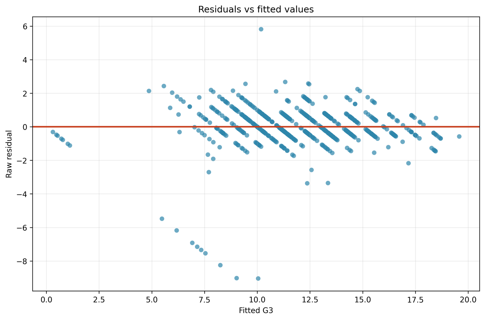
The point cloud is centered around the zero line, but the spread and local pattern are not fully uniform across fitted values. Integer-valued grades create visible bands, while extreme negative errors extend farther from zero than most positive errors.
The graph contains all 649 residuals from the model with R² = 0.850563 and RMSE = 1.253722. RESET is F = 9.868464, p = 0.001759; Breusch–Pagan and White p-values are 1.391 × 10⁻⁵ and 6.832 × 10⁻⁷.
Residual centering alone is not enough. The formal tests indicate that both the conditional-mean form and variance structure deserve review. Horizontal grade bands are expected for an integer outcome, but systematic curvature or changing envelope width is diagnostic.
This is the broadest first figure in Regression Residual Analysis. It directs the analyst toward nonlinear terms, robust uncertainty and closer inspection of the cases producing the largest negative residuals.
Python Chart 2: Normal Q–Q Plot
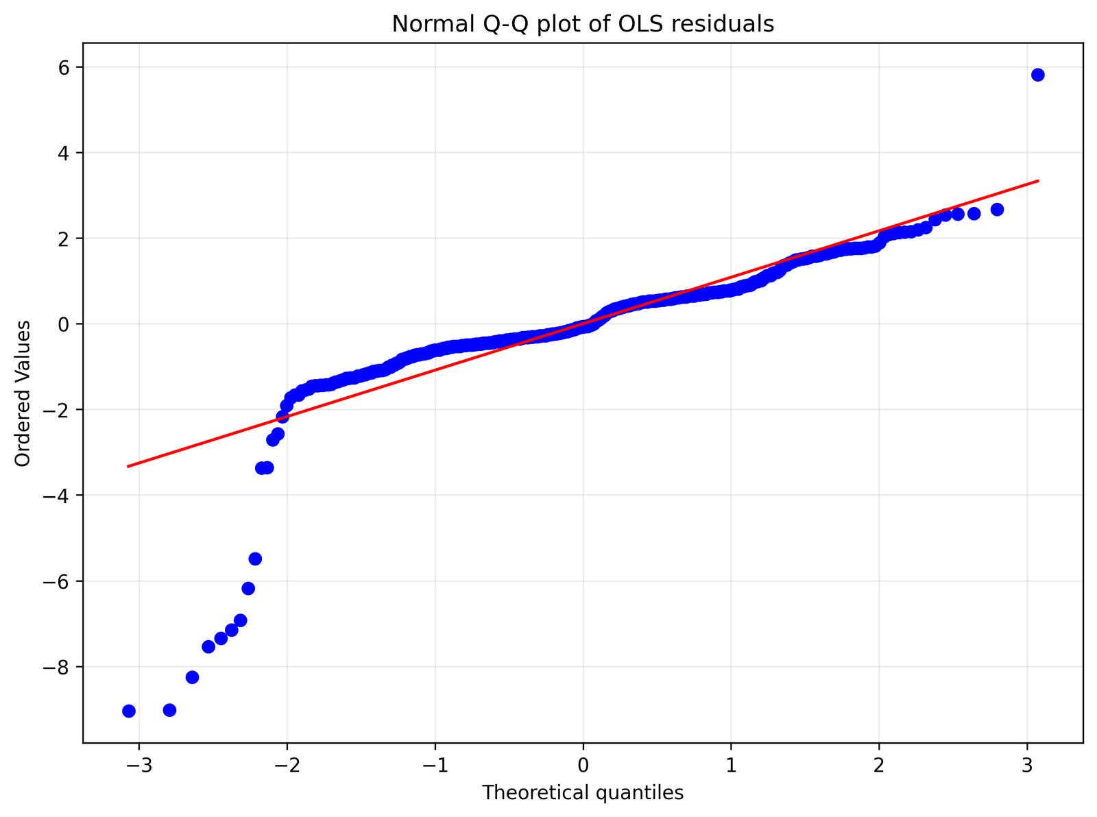
The central portion follows the reference line more closely than the tails. The most pronounced departure occurs in the lower tail, where several observations are much more negative than a normal residual model would predict.
Shapiro–Wilk is W = 0.756572 with p = 7.722 × 10⁻³⁰. Jarque–Bera is 10019.316610, with the p-value displayed as zero by the numerical output. The maximum absolute externally studentized residual is 7.581732.
The tail pattern is not a trivial cosmetic departure. It affects conventional small-sample reference assumptions and prediction intervals, even though OLS fitted values and slopes remain algebraically computable.
Regression Residual Analysis should respond by reporting the departure, checking source records for extreme cases, and considering HC3, bootstrap or other robust inference rather than deleting observations to force a straight Q–Q line.
Python Chart 3: Residual Histogram
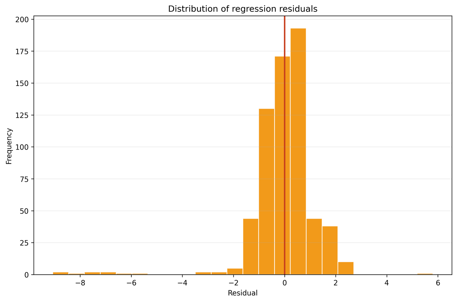
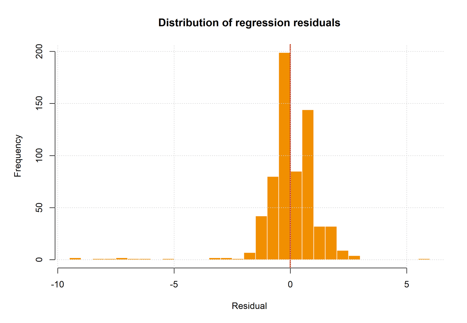
Most residuals are concentrated around zero, while a comparatively sparse but long negative tail creates strong asymmetry and excess tail weight. The center can look compact even when a few observations dominate formal normality tests.
The fitted model has RMSE = 1.253722. Ten observations exceed |externally studentized residual| > 3, and the largest absolute externally studentized residual is 7.581732.
The histogram explains why average error can remain modest while residual normality fails sharply. A small set of severe misses can coexist with accurate predictions for the majority of observations.
The figure matters for reporting prediction uncertainty and for deciding whether a robust or bounded-outcome approach should be compared. Bin width should not be used to hide the tail.
Python Chart 4: Scale–Location Plot
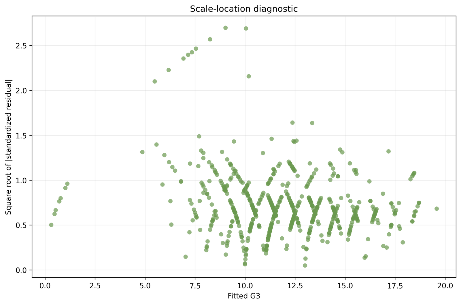
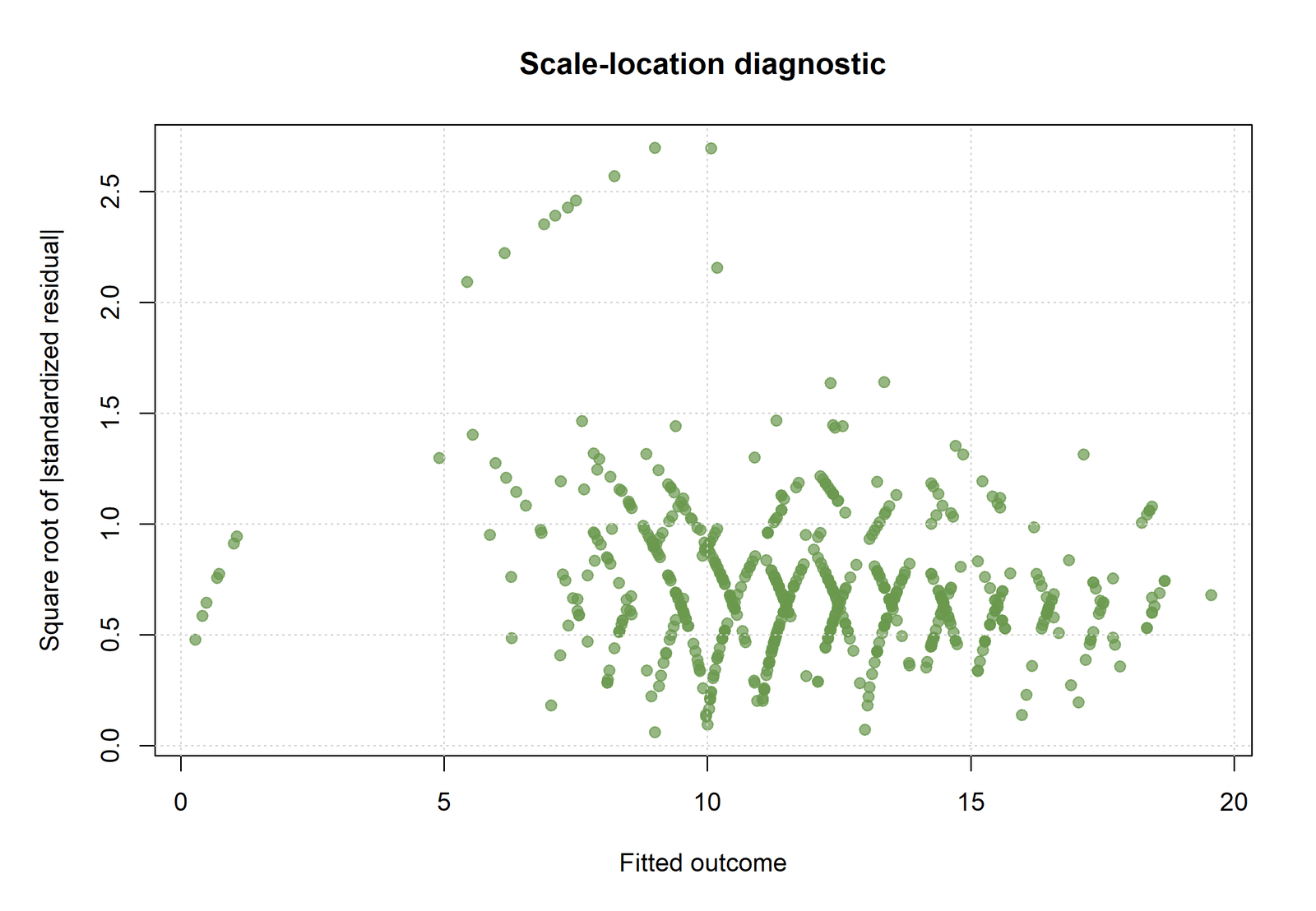
The vertical spread changes across the fitted-value range rather than forming a completely flat band. Because positive and negative signs are removed, changes in error magnitude are easier to see than in the ordinary residual plot.
Breusch–Pagan is 30.129021, p = 1.391 × 10⁻⁵. White is 66.454172, p = 6.832 × 10⁻⁷. Both tests independently flag nonconstant variance.
The conventional OLS coefficient estimates describe the fitted linear mean, but standard errors calculated under homoscedasticity may not reflect the observed variance pattern.
This Regression Residual Analysis result supports reporting HC3 or another justified robust covariance estimate and comparing whether substantive conclusions change. A variance remedy should be documented separately from a mean-structure remedy.
Python Chart 5: Studentized Residuals Versus Leverage
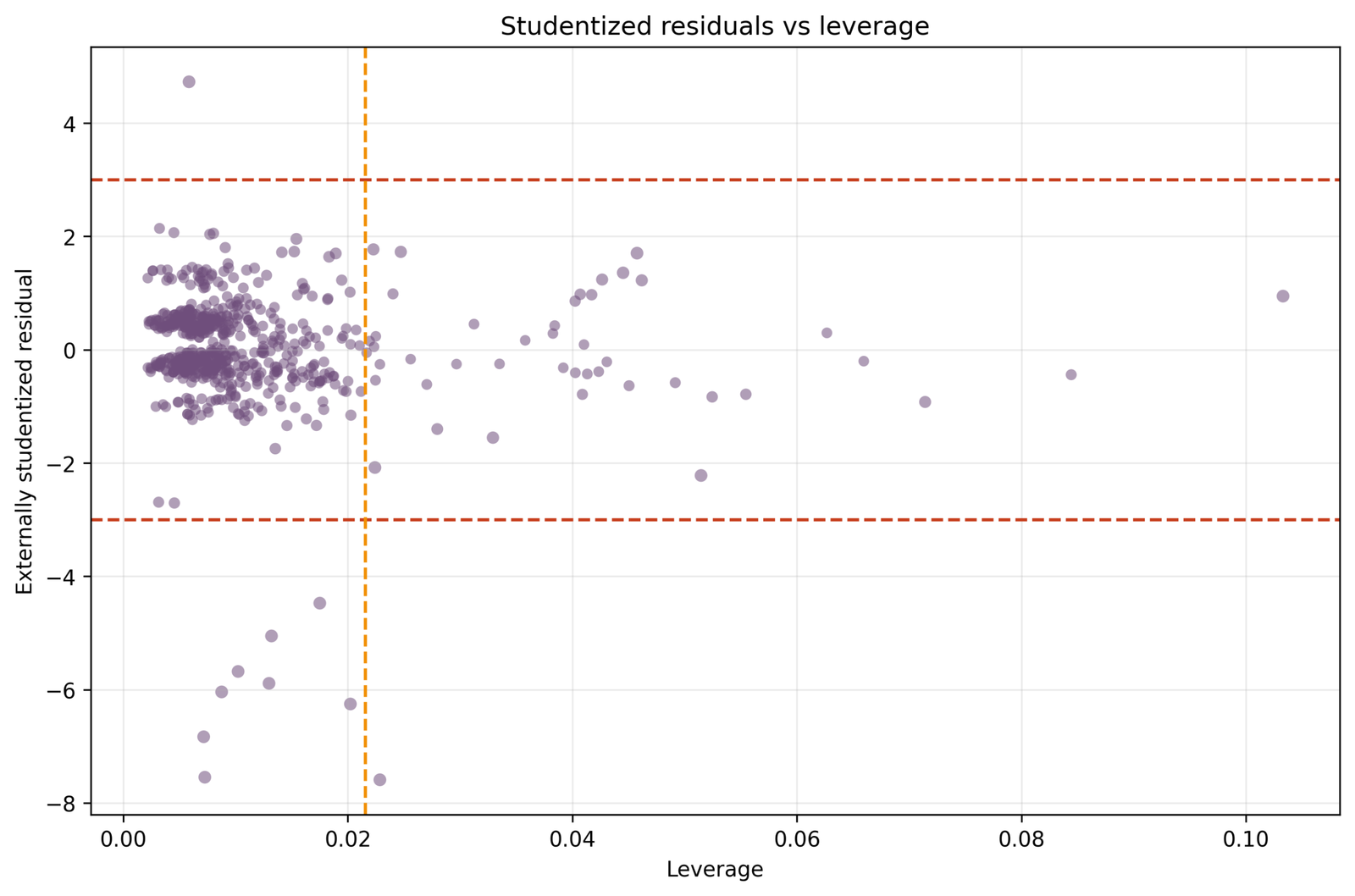
Most observations occupy the low-leverage central area, but several cases extend horizontally because their predictor profiles are unusual. Severe vertical departures identify response outliers; cases that are both horizontally and vertically unusual deserve the highest review priority.
The leverage review line is 0.01848998; 47 cases exceed it and the maximum leverage is 0.10328893. Ten cases exceed |deleted studentized residual| > 3. Case 1 has leverage 0.10328893 but deleted residual 0.947972.
High leverage is not the same as a large residual. Case 1 illustrates that a record can be unusual in predictor space and influence precision without being a response outlier.
Regression Residual Analysis uses this chart to separate mechanisms. Check coding and source values for high-leverage cases, then examine whether their deletion changes estimates before making any eligibility decision.
Python Chart 6: Cook’s Distance by Case
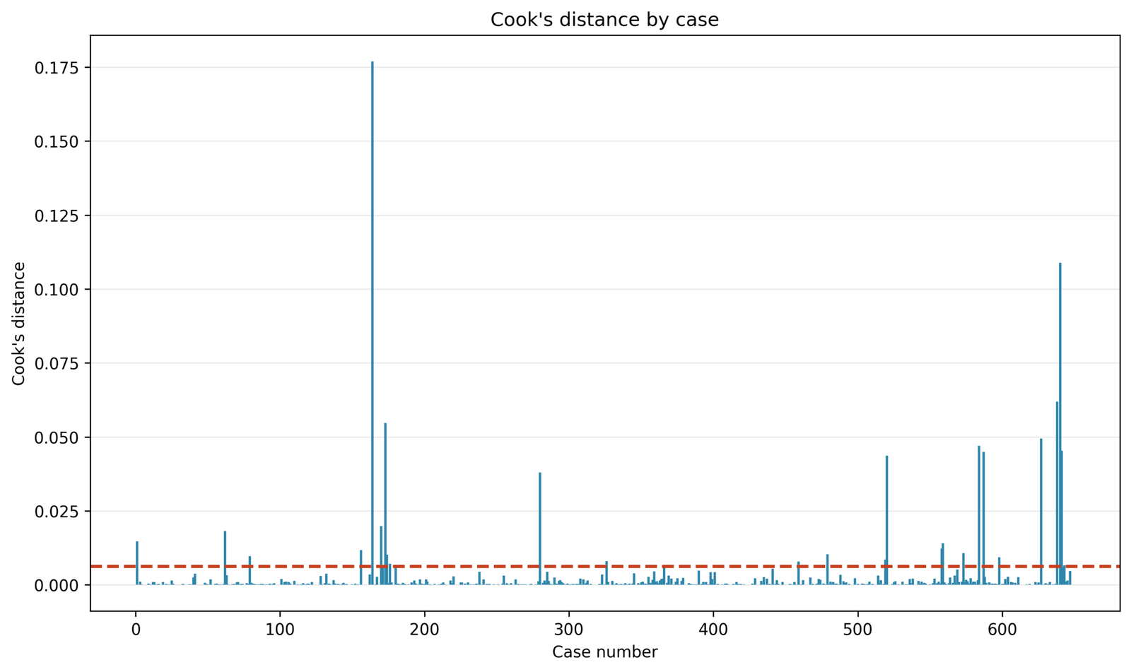
Most values are near zero, while a smaller group rises above the review line. The tallest value is visibly larger than the routine cases, but it remains a diagnostic priority rather than proof of invalid data.
The review line is 4/n = 0.00616333. Exactly 29 observations exceed it, and the maximum Cook’s distance is 0.20287792.
Cook’s distance combines residual magnitude and leverage to summarize joint coefficient influence. Two cases can have similar Cook’s distance for different combinations of outcome surprise and predictor rarity.
The figure matters because the coefficient table should be tested for sensitivity to the most influential verified cases. The primary model should remain intact unless a source or eligibility rule justifies exclusion.
Python Chart 7: Observed Versus Predicted G3
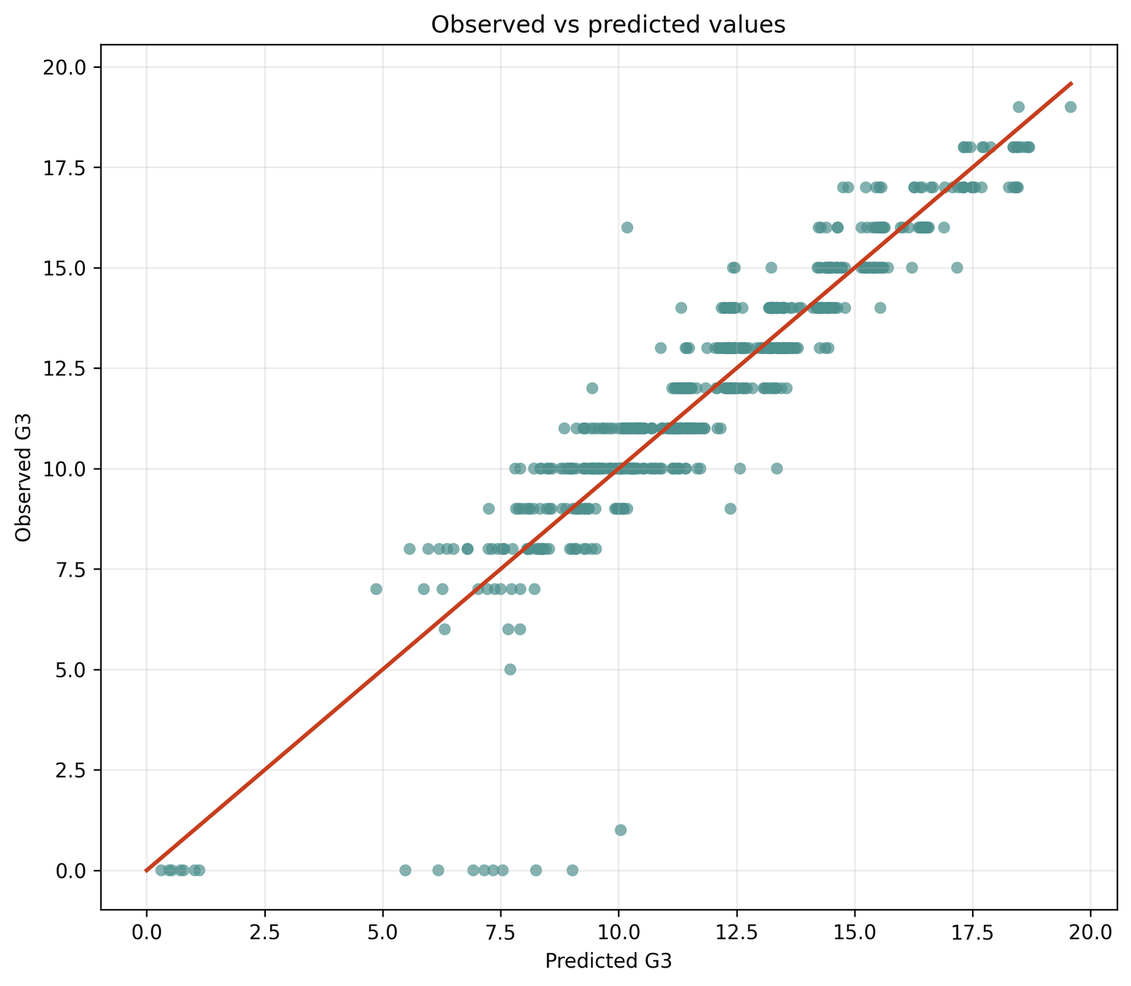
Most observations follow the increasing reference direction, especially through the dense middle range. Extreme low outcomes are harder for the linear mean to represent and contribute to the negative residual tail.
The fitted model explains 85.0563% of sample G3 variation, with adjusted R² = 0.849401 and RMSE = 1.253722. The overall model test is F(5,643) = 731.965860.
Strong calibration in the center can coexist with poor representation of boundary or exceptional outcomes. The plot supports the usefulness of the fitted mean but does not override the residual and variance conflicts.
Regression Residual Analysis places this figure beside residual plots so readers can see both the model’s practical strength and its tail limitations. External validation is still required before future-performance claims.
Python Chart 8: Standardized Residuals by Case
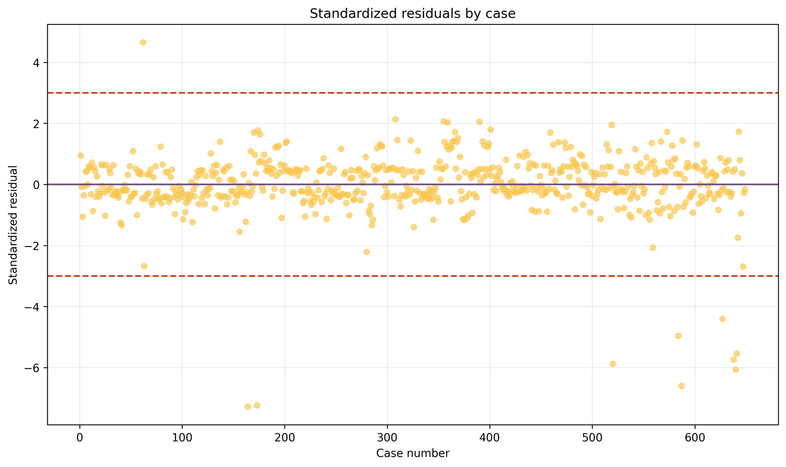
Most cases fluctuate near zero, but isolated negative spikes and a smaller number of positive spikes stand out. The sequence does not show an obvious smooth cycle, although row-order interpretation depends on how records were arranged.
Ten observations exceed the external-studentization rule of |tᵢ| > 3. Durbin–Watson is 1.857347, a value reasonably near two for the retained order.
The chart makes individual extreme errors visible and can reveal clustering in the ordering variable. It cannot establish independence unless the row sequence represents a meaningful temporal or spatial order.
This figure matters for tracing plotted spikes back to original records. Regression Residual Analysis should preserve row identifiers so every extreme point can be verified rather than guessed from its visual position.
Python Chart 9: Leverage Versus Absolute DFFITS
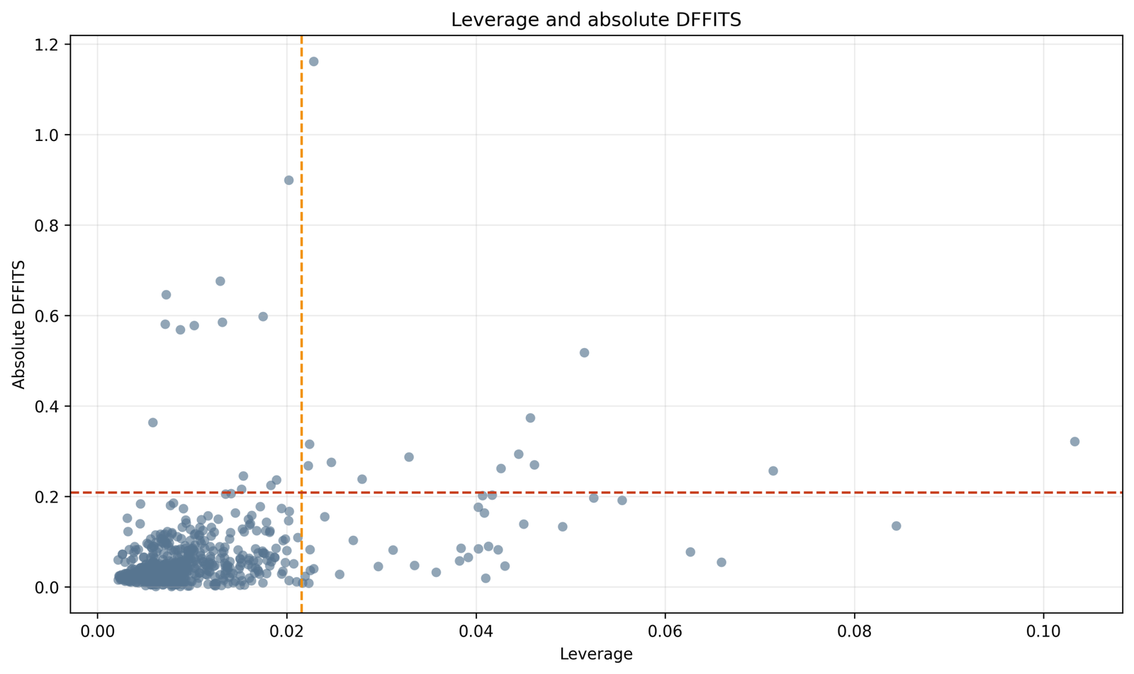
The majority of observations lie below both screening references. A smaller group combines high leverage with elevated absolute DFFITS, while some cases cross only one criterion.
The leverage threshold is 0.01848998. The absolute DFFITS threshold is 0.19230177. There are 47 leverage flags and 29 DFFITS flags; the maximum absolute DFFITS is 1.15073682.
Leverage describes potential to influence, whereas DFFITS records realized change in the focal fitted value under case deletion. A high-leverage point with a small residual may have modest DFFITS.
Regression Residual Analysis uses the joint display to prioritize multi-criterion cases for source review and sensitivity analysis. The two axes should not be collapsed into a single label such as “bad point.”
Python Chart 10: Coefficient Confidence Intervals
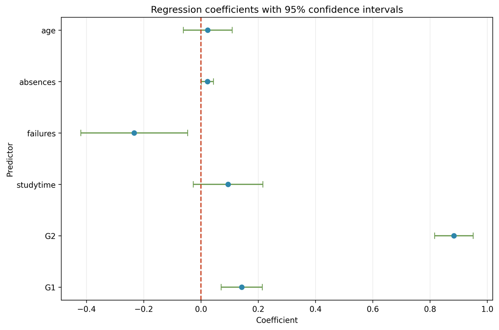
G2 has by far the largest positive adjusted slope and a narrow interval that does not cross zero. G1 is also positive. Failures is negative. Studytime crosses zero, while absences has a small positive interval under conventional OLS uncertainty.
G2: B = 0.885709, 95% CI [0.819088, 0.952329]. G1: B = 0.139457, 95% CI [0.0683, 0.2106]. Failures: B = −0.218290, 95% CI [−0.396711, −0.039870].
These are conditional associations from the declared model, not causal effects. Because both variance tests reject homoscedasticity, the conventional intervals should be compared with HC3 or another justified robust interval.
The chart connects Regression Residual Analysis back to substantive reporting. Diagnostics matter because they can change the uncertainty attached to the slopes even when point estimates and signs remain similar.
R Regression Residual Analysis Charts and Explanations
The R figures provide a same-topic visual cross-check using the identical outcome, predictor set and complete-case rule. They are displayed in paired rows, with one explanation box corresponding directly to each graph. Small numerical differences are acceptable only when residual definitions or plotting conventions are explicitly different.
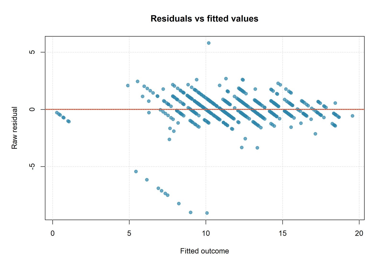
R Chart 1: Residuals Versus Fitted
Pattern: residuals remain broadly centered but do not form a perfectly uniform random band. Key values: R² = 0.850563, RESET p = 0.001759 and both variance-test p-values are below 0.001. Interpretation: the fitted mean is informative, yet curvature and changing variance remain plausible. Why it matters: inspect theory-supported nonlinear terms and robust uncertainty rather than using R² as an assumption check.
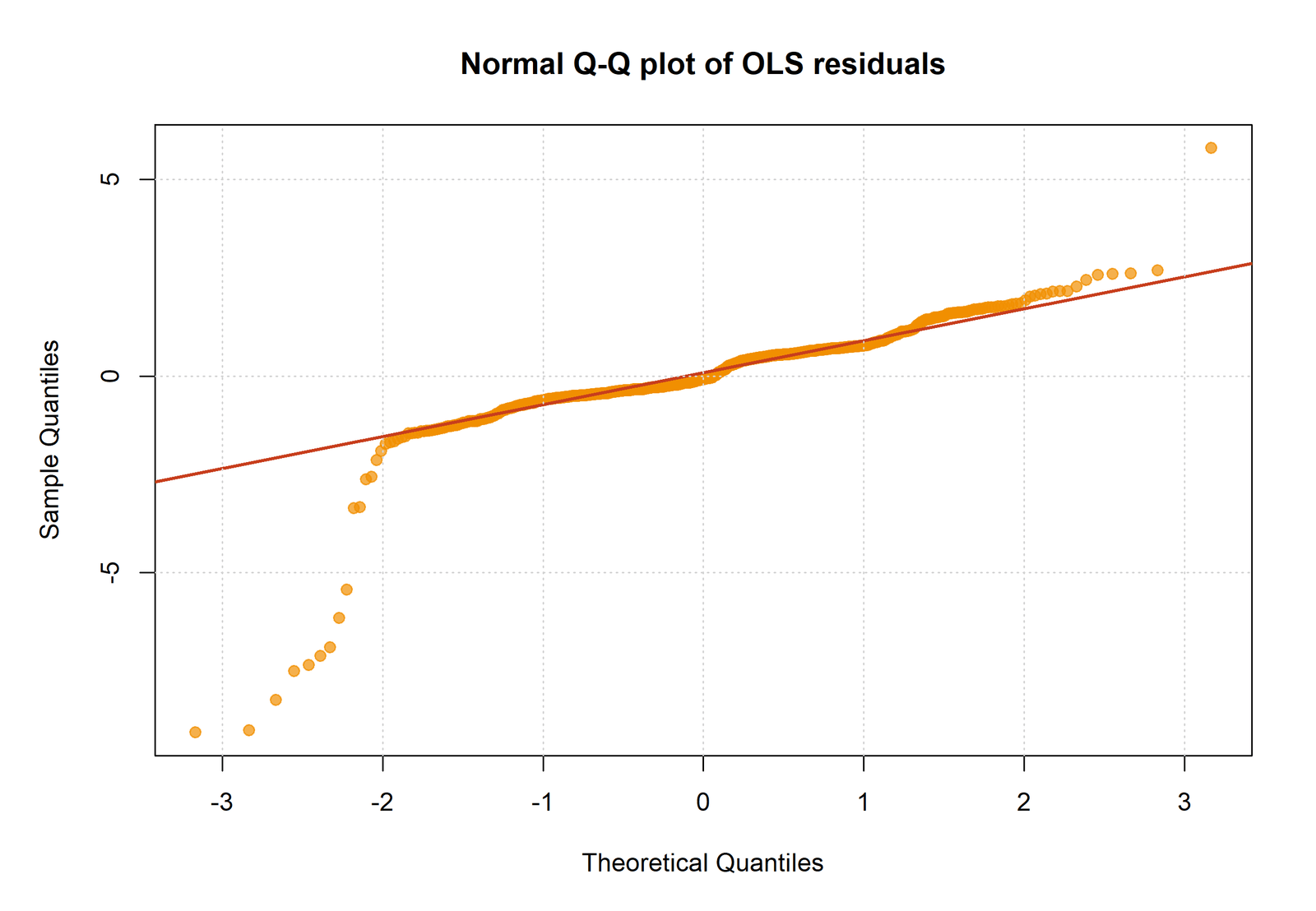
R Chart 2: Normal Q–Q Plot
Pattern: central points align better than the tails, with the strongest departure in the negative tail. Key values: Shapiro–Wilk W = 0.756572, p = 7.722 × 10⁻³⁰, and maximum |deleted residual| = 7.581732. Interpretation: normal-reference tail behavior is not supported. Why it matters: conventional tail-sensitive inference and individual prediction intervals require caution.
R Chart 3: Residual Histogram
Pattern: a compact central mass is accompanied by a long negative tail. Key values: RMSE = 1.253722, ten external-studentization flags and Jarque–Bera = 10019.316610. Interpretation: most observations are fitted reasonably, but a small tail contributes disproportionate non-normality. Why it matters: investigate the tail without redefining the sample around the model.
R Chart 4: Scale–Location Plot
Pattern: residual magnitude changes across fitted values instead of remaining flat. Key values: Breusch–Pagan = 30.129021, p = 1.391 × 10⁻⁵; White = 66.454172, p = 6.832 × 10⁻⁷. Interpretation: homoscedastic OLS uncertainty is not well supported. Why it matters: compare HC3 or another justified variance strategy before final interval reporting.
Regression Residual Analysis Coefficient Interpretation
The coefficient table defines the equation being diagnosed. Regression Residual Analysis does not replace coefficient interpretation; it determines how cautiously the conventional standard errors, confidence intervals and model form should be reported. Each slope is conditional on the other four included predictors and should not be treated as a causal effect.
| Term | B | SE | t | p | 95% conventional CI | Worked interpretation |
|---|---|---|---|---|---|---|
| Intercept | −0.155190 | 0.258626 | −0.6001 | 0.5487 | [−0.6630, 0.3527] | Expected G3 at zero on every predictor; this profile may have limited substantive meaning. |
| G1 | 0.139457 | 0.036227 | 3.8495 | 0.000130 | [0.0683, 0.2106] | A one-point higher G1 is associated with 0.139 higher fitted G3 when the other predictors are held constant. |
| G2 | 0.885709 | 0.033927 | 26.1066 | 5.438 × 10−103 | [0.8191, 0.9523] | G2 is the dominant positive adjusted predictor in the equation. |
| studytime | 0.096699 | 0.061810 | 1.5645 | 0.1182 | [−0.0247, 0.2181] | The linear one-code increase is not conventionally significant in this specification. |
| failures | −0.218290 | 0.090861 | −2.4025 | 0.0166 | [−0.3967, −0.0399] | Each additional prior failure is associated with a lower fitted G3 after adjustment. |
| absences | 0.023367 | 0.010794 | 2.1648 | 0.0308 | [0.0022, 0.0446] | The fitted association is small and positive; it should not be interpreted as a beneficial causal effect of absence. |
How the Diagnostics Affect Coefficient Reporting
The point estimates above are the OLS solution for the stated equation. Heteroscedasticity does not automatically bias those slopes under the standard exogeneity condition, but it can make homoscedastic standard errors and confidence intervals inappropriate. The significant RESET result also suggests that a coefficient may be averaging a relationship that changes across the predictor range. Therefore, a final report should compare conventional and HC3 uncertainty and should test any nonlinear specification selected from theory rather than from uncontrolled trial and error.
Predictions, Effects and Worked Residual Calculations
A fitted value is the conditional mean predicted by the five-predictor equation. Regression Residual Analysis begins only after that fitted value is calculated consistently. The worked case below demonstrates why prediction, residual, leverage and influence must be reported as separate quantities.
Worked Prediction for Case 1
| Term | Input | Coefficient | Contribution |
|---|---|---|---|
| Intercept | 1 | −0.155190 | −0.155190 |
| G1 | 0 | 0.139457 | 0.000000 |
| G2 | 11 | 0.885709 | 9.742799 |
| studytime | 2 | 0.096699 | 0.193398 |
| failures | 0 | −0.218290 | 0.000000 |
| absences | 4 | 0.023367 | 0.093468 |
| Predicted G3 | approximately 9.87447 | ||
The positive residual means the model underpredicted Case 1 by approximately 1.13 grade points. Its externally studentized residual is 0.947972, so it is not a residual outlier under the |t| > 3 rule. Its leverage is 0.103289, far above the 0.018490 review line, and its DFFITS is 0.321733. The case is therefore important because of its unusual predictor profile and influence, not because its observed G3 is extraordinarily far from the fitted value.
Prediction Versus Diagnostic Meaning
Prediction quantities
- Observed G3: the recorded outcome.
- Predicted G3: the fitted conditional mean.
- Raw residual: signed difference in grade points.
- RMSE: aggregate error scale across all cases.
Diagnostic quantities
- Studentized residual: case error relative to estimated spread.
- Leverage: rarity of the predictor combination.
- Cook’s distance: joint coefficient influence.
- DFFITS and COVRATIO: fitted-value and precision influence.
Regression Residual Analysis Assumptions and Diagnostic Decisions
The purpose of this section is to convert diagnostic evidence into explicit decisions. No single statistic can certify a model. Regression Residual Analysis is strongest when the graphical pattern, numerical test, case-level values and proposed remedy all point to the same mechanism.
| Diagnostic requirement | Worked evidence | Status | Defensible response |
|---|---|---|---|
| Linear conditional mean | RESET F = 9.868464, p = 0.001759; residual plot requires review | Potential issue | Investigate theory-supported nonlinear terms, interactions or splines and validate the alternative. |
| Constant residual variance | Breusch–Pagan p = 1.391 × 10⁻⁵; White p = 6.832 × 10⁻⁷ | Not supported | Report HC3 or another justified robust covariance; consider weighted or explicit variance modeling where appropriate. |
| Normal-reference residual tails | Shapiro–Wilk p = 7.722 × 10⁻³⁰; Jarque–Bera extremely large; Q–Q tail departure | Not supported | Use robust or resampling inference and avoid overconfident individual prediction intervals. |
| Approximate sequence independence | Durbin–Watson = 1.857347 | Reasonably near two for current order | Verify whether row order is meaningful and whether clustering or repeated observations exist. |
| No severe response outliers | 10 cases with |deleted residual| > 3; maximum = 7.581732 | Review required | Verify source records and retain valid observations in the primary analysis. |
| No influential design cases | 47 leverage, 29 Cook, 29 DFFITS and 49 COVRATIO flags | Review required | Prioritize multi-criterion cases and report documented sensitivity refits. |
Linearity and Functional Form
The RESET result rejects the simple claim that the five linear predictor terms completely capture the mean structure. This does not identify which variable needs transformation. Partial-residual plots, substantive theory and cross-validated comparison should guide whether to add polynomial, spline or interaction terms. A model should not be expanded until the p-value becomes nonsignificant by repeated searching.
Homoscedasticity
Both variance tests reject constant residual variance. The agreement is stronger evidence than either test alone, but the tests still do not select a remedy. HC3 uncertainty is often a reasonable first sensitivity analysis because it leaves the OLS mean equation unchanged. Weighted least squares is more demanding because weights must represent a defensible variance structure.
Residual Distribution
Residual normality is not required to calculate OLS slopes, and the central limit theorem can make coefficient inference relatively stable in large samples. However, the combination of extreme studentized residuals, a visibly abnormal tail and very strong normality-test results means that the issue should not be dismissed as sample-size sensitivity. Tail predictions and conventional prediction intervals require particular caution.
Independence
Durbin–Watson near two is reassuring only for first-order correlation in the retained order. If students are nested within classrooms or schools, or if records are repeated over time, a clustered or multilevel structure may remain even when Durbin–Watson appears acceptable. Study design takes priority over a single residual statistic.
Influence and Data Integrity
Sixty-six distinct observations cross at least one screening rule. A valid observation can be influential because it represents a rare but real predictor combination. The correct response is to compare the original record with the source, verify coding, and examine whether the central conclusions change in a clearly labeled sensitivity model. Deletion is justified by data quality or eligibility evidence, not by influence alone.
Regression Residual Analysis in Python, R, SPSS and Excel
Python
Use statsmodels OLS and its influence object to obtain fitted values, residual scales, leverage, Cook’s distance, DFFITS and COVRATIO. Use statsmodels diagnostic functions for RESET, Breusch–Pagan, White, Jarque–Bera and Durbin–Watson.
- Preserve an explicit case identifier.
- Export one case-level diagnostic table.
- State every threshold formula.
- Plot the exact residual vector used by the tests.
R
Fit the same equation with lm(). Use rstudent(), hatvalues(), cooks.distance(), dffits() and covratio(), together with appropriate diagnostic packages for formal checks.
- Confirm factor and numeric coding.
- Retain the intercept.
- Use identical complete rows.
- Document any residual-definition differences.
SPSS
Use REGRESSION to fit G3 on the five predictors and save predicted values, residuals, standardized or studentized residuals, leverage and Cook’s distance where available. Preserve the output viewer and case-level saved variables.
- Verify case order after import.
- Do not overwrite raw variables.
- Label saved diagnostic columns.
- Cross-check coefficient and model tables.
Excel
Use the supplied coefficients to calculate fitted values and raw residuals, then audit threshold formulas and Boolean flags. Excel is especially useful for transparent case-by-case review when the statistical quantities have already been generated correctly.
- Lock coefficient cells.
- Use full-precision calculations.
- Keep one row per original case.
- Separate data-error notes from statistical flags.
Code: Expand Only the Software You Need
Python Regression Residual Analysis code
import numpy as np
import pandas as pd
import statsmodels.api as sm
from statsmodels.stats.diagnostic import (
    linear_reset, het_breuschpagan, het_white
)
from statsmodels.stats.stattools import durbin_watson, jarque_bera
from scipy.stats import shapiro

predictors = ["G1", "G2", "studytime", "failures", "absences"]
work = data[["G3", *predictors]].dropna().copy()

X = sm.add_constant(work[predictors], has_constant="add")
fit = sm.OLS(work["G3"], X).fit()
infl = fit.get_influence()
frame = infl.summary_frame()

audit = work.reset_index(names="source_index")
audit["fitted"] = fit.fittedvalues.to_numpy()
audit["residual"] = fit.resid.to_numpy()
audit["studentized_deleted"] = infl.resid_studentized_external
audit["leverage"] = infl.hat_matrix_diag
audit["cooks_d"] = infl.cooks_distance[0]
audit["dffits"] = infl.dffits[0]
audit["covratio"] = infl.cov_ratio

n = len(audit)
p = X.shape[1]
audit["flag_studentized"] = audit["studentized_deleted"].abs() > 3
audit["flag_leverage"] = audit["leverage"] > 2 * p / n
audit["flag_cook"] = audit["cooks_d"] > 4 / n
audit["flag_dffits"] = audit["dffits"].abs() > 2 * np.sqrt(p / n)
audit["flag_covratio"] = (
    (audit["covratio"] < 1 - 3 * p / n) |
    (audit["covratio"] > 1 + 3 * p / n)
)
flag_cols = [c for c in audit if c.startswith("flag_")]
audit["flag_any"] = audit[flag_cols].any(axis=1)

reset = linear_reset(fit, power=2, use_f=True)
bp = het_breuschpagan(fit.resid, fit.model.exog)
white = het_white(fit.resid, fit.model.exog)
dw = durbin_watson(fit.resid)
jb = jarque_bera(fit.resid)
sw = shapiro(fit.resid)
Keep preprocessing and case identifiers explicit. The exact field names returned by an influence summary may differ by statsmodels version, so verify each column before publication.
R Regression Residual Analysis code
vars <- c("G3", "G1", "G2", "studytime", "failures", "absences")
work <- na.omit(data[vars])
fit <- lm(G3 ~ G1 + G2 + studytime + failures + absences, data = work)

n <- nrow(work)
p <- length(coef(fit))

audit <- transform(
  work,
  fitted = fitted(fit),
  residual = resid(fit),
  studentized_deleted = rstudent(fit),
  leverage = hatvalues(fit),
  cooks_d = cooks.distance(fit),
  dffits = dffits(fit),
  covratio = covratio(fit)
)

audit$flag_studentized <- abs(audit$studentized_deleted) > 3
audit$flag_leverage <- audit$leverage > 2 * p / n
audit$flag_cook <- audit$cooks_d > 4 / n
audit$flag_dffits <- abs(audit$dffits) > 2 * sqrt(p / n)
audit$flag_covratio <- audit$covratio < (1 - 3*p/n) |
                       audit$covratio > (1 + 3*p/n)

plot(fit, which = 1)
qqnorm(resid(fit)); qqline(resid(fit))
hist(resid(fit), main = "Residual histogram", xlab = "Residual")
Additional packages can provide RESET and heteroscedasticity tests. Record package versions and do not assume that identically named residuals are calculated with identical small-sample conventions.
SPSS Regression Residual Analysis syntax
REGRESSION
  /DEPENDENT G3
  /METHOD=ENTER G1 G2 studytime failures absences
  /STATISTICS COEFF OUTS R ANOVA CI(95)
  /RESIDUALS DURBIN HISTOGRAM(ZRESID) NORMPROB(ZRESID)
  /CASEWISE PLOT(ZRESID) OUTLIERS(3)
  /SAVE PRED RESID ZRESID SRESID LEVER COOK.
Saved-variable names can vary. Inspect the active dataset after execution, retain the original case identifier and export the output viewer as the audit record.
Excel formulas for fitted values and flags
Predicted G3:
=$B$2+$B$3*[@G1]+$B$4*[@G2]+$B$5*[@studytime]
+$B$6*[@failures]+$B$7*[@absences]

Raw residual:
=[@G3]-[@[Predicted G3]]

Studentized flag:
=ABS([@[Deleted Studentized Residual]])>3

Leverage flag:
=[@Leverage]>(2*6/649)

Cook flag:
=[@[Cook Distance]]>(4/649)

DFFITS flag:
=ABS([@DFFITS])>(2*SQRT(6/649))

COVRATIO flag:
=OR([@COVRATIO]<(1-3*6/649),[@COVRATIO]>(1+3*6/649))

Any flag:
=OR([@[Studentized Flag]],[@[Leverage Flag]],[@[Cook Flag]],
    [@[DFFITS Flag]],[@[COVRATIO Flag]])
Use full-precision diagnostic values in hidden or calculation columns and format the visible cells separately. Rounding before applying thresholds can change borderline flags.
26 Advanced Regression Residual Analysis Topics
These expandable panels extend the worked analysis from basic residual interpretation to robust inference, model revision, validation and reproducible case review. Open only the topics needed for the current reporting decision.
1. Regression Residual Analysis: Raw Residuals and Sign Direction
A raw residual is observed G3 minus fitted G3. Positive values indicate underprediction and negative values indicate overprediction. The residual retains the outcome unit, making it easy to explain but difficult to compare across observations with different leverage.
In an OLS model with an intercept, residuals sum to approximately zero and are orthogonal to the included predictor columns. Those algebraic facts do not prove that the residual pattern is random or that the model is correctly specified.
Caution: Do not call a negative residual a negative outcome effect; it is simply an overprediction under the fitted equation.
2. Regression Residual Analysis: Internally Standardized Versus Externally Studentized Residuals
Internally standardized residuals use the model’s overall residual spread, including the focal case. Externally studentized residuals estimate the spread after deleting that case. The deleted version can reveal a severe outlier that partially masks itself by inflating the full-sample error estimate.
The worked Regression Residual Analysis uses |externally studentized residual| > 3 as a review rule. Ten cases cross it, and the maximum absolute value is 7.581732.
Caution: A threshold crossing requests verification; it does not establish fabrication, miscoding or exclusion eligibility.
3. Regression Residual Analysis: The Hat Matrix and Leverage
The hat matrix H maps observed outcomes to fitted values. Its diagonal hᵢᵢ measures how far a predictor profile lies from the center of the design space. Leverage depends on X, not on the observed G3 value.
With p = 6 fitted coefficients and n = 649, the worked review line is 2p/n = 0.01848998. Forty-seven observations exceed it, and the maximum is 0.10328893.
Caution: Leverage is not an error measure. A perfectly recorded case can have high leverage because it represents a rare but valid predictor profile.
4. Regression Residual Analysis: Cook’s Distance
Cook’s distance summarizes the joint effect of deleting one case on the fitted coefficient vector. It increases when residual magnitude, leverage or both are substantial. The conventional 4/n line equals 0.00616333 in this analysis.
Twenty-nine cases exceed the line and the maximum Cook’s distance is 0.20287792. The line is intentionally sensitive in a large sample and should be treated as a screen.
Caution: Do not delete all observations above 4/n. That practice can remove a legitimate part of the population and manufacture apparent assumption compliance.
5. Regression Residual Analysis: DFFITS
DFFITS measures the standardized change in an observation’s fitted value when that observation is deleted. It therefore focuses on prediction at the focal design point rather than the complete coefficient vector.
The worked threshold is 2√(p/n) = 0.19230177. Twenty-nine cases exceed it and the maximum absolute DFFITS is 1.15073682.
Caution: DFFITS and Cook’s distance are related but not interchangeable; report the quantity that matches the influence question.
6. Regression Residual Analysis: DFBETAS for Individual Slopes
DFBETAS quantify how much each coefficient changes, in standard-error units, when a case is omitted. They answer which specific slope is sensitive, whereas Cook’s distance summarizes joint influence.
A case can have moderate Cook’s distance yet strongly affect one coefficient if its predictor profile aligns with that term. DFBETAS are especially valuable when the research conclusion focuses on G2, failures or another named predictor.
Caution: Because no verified DFBETAS table was supplied in the attached results, do not invent case counts or maxima for this measure.
7. Regression Residual Analysis: COVRATIO
COVRATIO compares the determinant of the coefficient covariance matrix with and without a case. Values below one can indicate reduced precision after deletion; values above one can indicate increased precision, depending on the design and residual contribution.
The worked interval is 0.97226502 to 1.02773498, and 49 cases lie outside it. This is the largest individual flag count in the supplied analysis.
Caution: A COVRATIO flag does not necessarily imply a large change in prediction or coefficient direction.
8. Regression Residual Analysis: PRESS Residuals and Leave-One-Out Prediction
A PRESS residual predicts each observation from a model fitted without that observation. It is closely related to leverage-adjusted residuals and provides a leave-one-out view of prediction error. PRESS can reveal optimistic fitted-sample performance that ordinary residuals conceal.
The current article reports fitted RMSE and case-deletion diagnostics but does not claim a verified PRESS statistic. A future prediction-focused extension should calculate PRESS or nested cross-validation without changing the primary diagnostic findings.
Caution: Do not describe R² = 0.850563 as future predictive accuracy.
9. Regression Residual Analysis: Residuals Versus Fitted Values
This graph is the broad first check for curvature, changing spread and unusual errors. A smooth curve around zero suggests missing nonlinear mean structure. A funnel suggests heteroscedasticity. Integer-valued outcomes can produce bands without automatically violating the model.
In the worked analysis, the plot is interpreted with RESET p = 0.001759 and two highly significant variance tests.
Caution: Do not fit a complicated curve solely because a smoother is not perfectly horizontal in a large sample.
10. Regression Residual Analysis: Normal Q–Q Plot and Residual Histogram
The Q–Q plot emphasizes quantile departure, while the histogram emphasizes overall shape. They are complementary because a histogram can hide tail behavior through bin choice and a Q–Q plot can make the center appear satisfactory while extremes depart sharply.
Shapiro–Wilk W = 0.756572 and Jarque–Bera = 10019.316610 agree with the strong lower-tail pattern.
Caution: Normality tests become highly sensitive as n grows; interpret effect size, tail severity and inferential purpose, not p-values alone.
11. Regression Residual Analysis: Scale–Location Plot
The scale–location graph usually plots √|standardized residual| against fitted values. Removing the residual sign prevents positive and negative errors from canceling visually and makes variance trends easier to detect.
The worked plot is supported by Breusch–Pagan p = 1.391 × 10⁻⁵ and White p = 6.832 × 10⁻⁷.
Caution: A scale-location trend identifies a variance problem; it does not estimate correct weights by itself.
12. Regression Residual Analysis: Ramsey RESET Specification Test
RESET adds powers or functions of the fitted values to test whether the original linear predictor may omit nonlinear structure. The worked F statistic is 9.868464 with p = 0.001759.
A significant result indicates misspecification risk but does not identify the omitted variable, interaction or transformation. It can also react to heteroscedasticity or other departures.
Caution: Do not add arbitrary polynomial terms until RESET becomes nonsignificant.
13. Regression Residual Analysis: Breusch–Pagan Test
The Breusch–Pagan test examines whether squared residual variation is associated with the supplied design. The statistic is 30.129021 with p = 1.391 × 10⁻⁵, providing evidence against constant variance.
The test is most interpretable when the auxiliary variance relationship is plausibly linear in the predictors.
Caution: A significant Breusch–Pagan test does not mean the OLS point estimates should automatically be discarded.
14. Regression Residual Analysis: White Test
The White test allows a broader auxiliary variance pattern, often including squares and cross-products of regressors. The worked statistic is 66.454172 with p = 6.832 × 10⁻⁷.
Agreement with Breusch–Pagan strengthens the conclusion that residual variance is not constant, although the White test can consume many degrees of freedom in smaller datasets.
Caution: Do not infer the exact variance function from the White test alone.
15. Regression Residual Analysis: Durbin–Watson and Observation Order
Durbin–Watson = 1.857347 is reasonably close to two for the retained row order. It primarily targets first-order residual autocorrelation and is meaningful only when adjacent rows represent a relevant sequence.
Cross-sectional educational data may be clustered by school or classroom even when arbitrary file order produces an acceptable Durbin–Watson value.
Caution: Do not write that independence is proven because Durbin–Watson is near two.
16. Regression Residual Analysis: Bounded Outcomes, Floor Effects and Ceiling Effects
G3 has a bounded practical range, while a linear model can predict any real number. Near a lower or upper boundary, residual variance can compress and the conditional mean can become nonlinear. A cluster of zero grades can create a pronounced negative tail when predictor histories imply higher expected performance.
Caution: Do not choose a new model solely to remove difficult observations; the alternative must match the outcome scale and estimand.
17. Regression Residual Analysis: Heteroscedasticity-Consistent Standard Errors
HC0 through HC3 covariance estimators leave OLS coefficients and fitted values unchanged but adjust coefficient uncertainty for nonconstant variance. HC3 gives stronger leverage correction and is often preferred for finite-sample sensitivity reporting.
The attached results establish heteroscedasticity but do not provide verified HC3 intervals, so this article recommends the comparison without inventing numerical robust results.
Caution: Robust standard errors do not repair nonlinearity, omitted variables, clustering or extreme prediction error.
18. Regression Residual Analysis: Weighted Least Squares
Weighted least squares changes the estimation criterion so observations with larger modeled variance receive less weight. It can improve efficiency when a defensible variance function is known or estimated reliably.
Unlike robust covariance, WLS changes coefficients, fitted values and residuals. A complete Regression Residual Analysis must therefore be rerun for the weighted model.
Caution: Data-dependent weights can overfit the same residual pattern they are intended to correct.
19. Regression Residual Analysis: Transformations, Polynomials, Interactions and Splines
The significant RESET result motivates a structured search for mean-form improvements. Transformations may linearize a relationship; polynomial terms represent smooth curvature; interactions allow one predictor’s association to vary with another; splines provide flexible local shape.
Caution: Repeatedly testing many forms until diagnostics look favorable inflates researcher degrees of freedom.
20. Regression Residual Analysis: Robust Regression
Robust regression changes the loss function so extreme residuals have less influence. It can reveal whether the central coefficient pattern persists when tail observations receive reduced weight.
Robust regression estimates a different fitted solution from OLS and should be presented as a sensitivity or alternative estimand, not as a hidden cleanup step.
Caution: Downweighting a valid rare subgroup can conceal meaningful heterogeneity.
21. Regression Residual Analysis: Clustered and Multilevel Residual Structure
Observations nested within classrooms, schools, families or repeated students can share unmodeled variation. Ordinary residual plots may look acceptable while standard errors remain too small because independence is violated at the cluster level.
Caution: Durbin–Watson does not diagnose arbitrary cluster dependence.
22. Regression Residual Analysis: Large Samples, Multiple Tests and Practical Importance
With 649 observations, small departures can become statistically detectable. At the same time, the very large Jarque–Bera value, ten extreme studentized residuals and agreement between two heteroscedasticity tests indicate that the current concerns are not based on one marginal p-value.
Caution: Do not treat every p < .05 as requiring a different model, and do not dismiss every significant result as mere sample-size sensitivity.
23. Regression Residual Analysis: Case Deletion and Sensitivity Analysis
A sensitivity analysis asks whether conclusions change under a documented alternative, such as correcting a confirmed data error or temporarily omitting a small set of the most influential verified observations. It is not a license to select the cleanest result.
The primary model in this article retains all 649 complete cases. The 66 flagged observations form a review list, not a deletion list.
Caution: Never remove all flagged cases as a single automatic batch.
24. Regression Residual Analysis: Cross-Validation and External Validation
Residual diagnostics evaluate the fitted model on the analyzed sample. Cross-validation and external validation evaluate performance on observations not used to estimate the same coefficients. A model can have attractive residual plots yet generalize poorly, or have imperfect residual normality while predicting well.
Caution: Do not use the current fitted R² or RMSE as evidence of out-of-sample performance.
25. Regression Residual Analysis: Python, R, SPSS and Excel Reconciliation
Software can differ in definitions of standardized residuals, deleted residuals, leverage-adjusted scales, case indexing and small-sample test formulas. Agreement requires matching the equation, rows, intercept, precision and definitions.
Caution: Do not average conflicting outputs or assume one program is correct because it is more familiar.
26. Regression Residual Analysis: Audit Trail and Reproducible Reporting
A publishable Regression Residual Analysis should preserve the raw-data identifier, analysis formula, missing-data rule, software version, coefficient table, case-level diagnostic ledger, threshold formulas, plots, formal tests and every sensitivity decision. This record protects against selective interpretation and makes future correction possible.
Caution: Do not overwrite the original output with a revised model or cleaned dataset.
APA-Style Reporting for Regression Residual Analysis
A multiple linear regression predicted G3 from G1, G2, studytime, failures and absences using 649 complete observations. The model was statistically significant, F(5, 643) = 731.97, p < .001, and explained 85.06% of the fitted-sample variance in G3, R2 = .851, adjusted R2 = .849, RMSE = 1.254. G2 was the strongest positive adjusted predictor, B = 0.886, 95% CI [0.819, 0.952], p < .001; G1 was also positive, B = 0.139, 95% CI [0.068, 0.211], p < .001; and failures was negative, B = −0.218, 95% CI [−0.397, −0.040], p = .017.
Regression Residual Analysis identified possible functional-form error, RESET F = 9.87, p = .002, and heteroscedasticity by both Breusch–Pagan, statistic = 30.13, p < .001, and White, statistic = 66.45, p < .001, tests. Residual normality was not supported, Shapiro–Wilk W = .757, p < .001, and ten observations exceeded |externally studentized residual| > 3. Forty-seven observations crossed the leverage screen, 29 crossed Cook’s-distance and DFFITS screens, 49 crossed the COVRATIO band, and 66 unique observations met at least one review criterion. These observations were treated as diagnostic review cases rather than automatically excluded. Robust uncertainty, theory-guided functional-form assessment and documented sensitivity analysis were recommended.
Regression Residual Analysis Publication Checklist
Model and data
- State the exact formula and intercept convention.
- Name G3 as the outcome and all five predictors.
- Report N = 649 and the complete-case rule.
- Preserve a stable case identifier.
- Report R², adjusted R², F, p and RMSE.
- Provide the complete coefficient table with units.
- Distinguish fitted-sample and validation performance.
- Describe study design and possible clustering.
Diagnostics and decisions
- Define raw residual sign.
- Identify standardized versus externally studentized residuals.
- Show the formula for every screening threshold.
- Report flag counts and the 66-case union correctly.
- Link each chart to exact numerical evidence.
- Do not label flags as invalid data.
- Report robust or sensitivity analyses separately.
- Archive the original full-data result.
Downloads and Regression Residual Analysis Chart Resources
SPSS Regression Residual Analysis OutputSaved SPSS model and residual diagnostic evidence.
Worked Excel Residual WorkbookFitted values, residuals, thresholds, case flags and auditable formulas.
Python Diagnostic Chart StoriesJump to all ten figures with exact Pattern, Key Values, Interpretation and Why It Matters explanations.
Paired R Diagnostic ChartsOpen the four R visuals and their corresponding explanation boxes.
Software Code PanelsOpen the Python, R, SPSS and Excel implementation examples.
Direct Internal Chart Files
Frequently Asked Questions About Regression Residual Analysis
1. What is Regression Residual Analysis?
Regression Residual Analysis is the structured examination of observed-minus-predicted errors, residual assumptions and case influence after a regression model is fitted. It connects plots, formal tests and case-level evidence to a documented modeling decision.
2. What is the formula for a raw residual?
The raw residual for case i is eᵢ = yᵢ − ŷᵢ. In this post, yᵢ is observed G3 and ŷᵢ is the value predicted from G1, G2, studytime, failures and absences.
3. What does a positive or negative residual mean?
A positive residual means observed G3 is above the fitted value, so the model underpredicted that case. A negative residual means the fitted value is above observed G3, so the model overpredicted it.
4. What is the difference between standardized and studentized residuals?
Both scale residuals by estimated spread and leverage. An externally studentized residual uses an error estimate calculated with the focal case deleted, which makes it particularly useful for detecting observations that mask their own extremeness.
5. Does |studentized residual| greater than 3 prove bad data?
No. It is a screening convention. The ten flagged observations require source verification and substantive review, but they remain valid unless an eligibility or data-quality rule shows otherwise.
6. What is leverage in Regression Residual Analysis?
Leverage measures how unusual a case’s predictor combination is. It depends on the design matrix rather than the observed outcome. The worked line is 0.01848998, 47 cases exceed it and the maximum is 0.10328893.
7. What does Cook’s distance measure?
Cook’s distance combines residual size and leverage to summarize how deleting a case affects the fitted coefficient vector. Twenty-nine cases exceed 4/n = 0.00616333 in the worked model.
8. What does DFFITS measure?
DFFITS measures the standardized change in a case’s fitted value when that case is omitted. The worked absolute threshold is 0.19230177, with 29 cases flagged and a maximum absolute value of 1.15073682.
9. What does COVRATIO measure?
COVRATIO describes how deleting a case changes the determinant of the coefficient covariance matrix. Forty-nine observations fall outside the worked band from 0.97226502 to 1.02773498.
10. Why are there 66 unique flags when the category counts total more?
The flag categories overlap. One observation can exceed leverage, Cook’s distance, DFFITS and COVRATIO rules simultaneously. Sixty-six is the union of distinct cases with at least one flag.
11. Must residuals be perfectly normal?
No. Perfect normality is not required to compute OLS coefficients. Normal-reference behavior matters more for conventional small-sample inference and prediction intervals. The severe tail evidence here still warrants robust or resampling checks.
12. Why use both Breusch–Pagan and White tests?
They examine nonconstant variance under different auxiliary structures. Both reject homoscedasticity in this model, strengthening the warning, but neither identifies the correct variance remedy by itself.
13. Does Durbin–Watson = 1.857347 prove independence?
No. It is reasonably close to two for the retained order, but independence depends on data collection, clustering and meaningful sequence. Classroom, school or repeated-measure dependence requires design-specific methods.
14. Do robust standard errors fix the model?
No. HC3 or another robust covariance can improve uncertainty estimates under heteroscedasticity, but it does not change the fitted mean, repair nonlinear form, correct data errors or model clustering.
15. What does the significant Ramsey RESET result mean?
RESET F = 9.868464, p = 0.001759 indicates that the additive linear mean structure may omit nonlinear information. It does not specify which term to add; theory and validated model comparison must guide revision.
16. Which Regression Residual Analysis charts should be reported?
At minimum, report residuals versus fitted, a Q–Q or distribution plot, a scale-location or variance display, and an influence plot. This worked post adds observed-versus-predicted, case-sequence, DFFITS and coefficient-interval figures for a complete audit.
Regression Residual Analysis Conclusion
Regression Residual Analysis changes the interpretation of this five-predictor grade model without erasing its strengths. The equation explains approximately 85.06% of fitted-sample G3 variation and has RMSE = 1.253722, so G1, G2, studytime, failures and absences provide a highly informative conditional mean. G2 is the dominant positive predictor, G1 is also positive, and failures has a negative adjusted association.
The remaining evidence prevents an unqualified “assumptions satisfied” conclusion. RESET indicates potential functional-form error, both Breusch–Pagan and White tests identify heteroscedasticity, normality checks show severe tail departure, and 66 distinct cases meet at least one residual, leverage or influence screen. Durbin–Watson is reasonably near two for the retained order, but study-design independence must still be verified.
The correct next step is not to delete all flagged observations or abandon regression. Retain the full 649-case result as the primary analysis, verify the most influential source records, calculate robust uncertainty, investigate a limited theory-supported nonlinear specification, and report sensitivity findings transparently. That approach uses Regression Residual Analysis as a scientific quality-control process rather than a cosmetic search for perfect plots.

