
Robust Regression: Huber Formula, Weights, Interpretation, Python, R, SPSS and Excel
Robust Regression estimates a linear relationship while limiting the effect of observations with unusually large residuals. This complete worked guide compares ordinary least squares, Huber M-estimation and Tukey biweight estimation for 649 student records, interprets the coefficients and case weights, and connects the verified Python, R, SPSS and Excel evidence.
Robust Regression Model Overview
Robust Regression is a family of regression estimators designed to describe a conditional relationship without allowing a small number of extreme residuals to dominate the fitted coefficients. The method answers a practical question: what linear association is supported by the central pattern of the data when observations that conflict strongly with the fitted equation are given bounded influence rather than unlimited squared-error influence?
Use Robust Regression when the outcome is continuous, the intended mean structure is linear in the selected predictors, and ordinary least squares may be sensitive to vertical outliers or heavy-tailed errors. It is especially valuable when valid unusual observations should remain visible in the analysis rather than being deleted through an arbitrary cutoff. A robust estimator is not automatically required whenever a residual is large; it is justified when coefficient stability and resistance to residual extremes matter for the research question.
Ordinary least squares minimizes the sum of squared residuals, so each residual becomes increasingly influential as its magnitude grows. Robust Regression replaces that unrestricted quadratic loss with a loss function whose tail contribution grows more slowly. In the primary Huber model, small standardized residuals retain full weight and large standardized residuals receive progressively smaller weights. Iteratively reweighted least squares repeatedly updates those weights and refits the same linear equation until the coefficients stabilize.
A Robust Regression coefficient is interpreted on the original outcome scale. Holding the other predictors constant, the Huber coefficient for G2 of 0.8650 means that a one-point increase in G2 is associated with an estimated 0.865-point increase in the conditional Robust Regression prediction for G3. This is an adjusted association, not a causal effect. Robust Regression predictions use the fitted robust coefficients, while the case weights describe how strongly each observation contributed during estimation; the weights are not predicted probabilities or survey weights.
Robust Regression differs from several related tools. Heteroscedasticity-consistent standard errors keep the OLS coefficients and change only their uncertainty. Weighted least squares uses externally motivated precision weights rather than residual-based influence weights. Quantile regression estimates a conditional quantile instead of a conditional mean. Student-t regression specifies a heavy-tailed probability model, whereas Huber M-estimation uses an estimating equation. Tukey biweight is more aggressive than Huber because sufficiently extreme standardized residuals can receive zero weight.
The method supports continuous outcomes and numeric or appropriately coded categorical predictors, interactions and nonlinear basis terms. Its core assumptions remain important: the chosen conditional mean must be substantively meaningful, observations should be independent at the modeled sampling level, predictor coding must be correct, and important leverage or clustering structures cannot be ignored. Robust Regression reduces sensitivity to vertical residual extremes, but it does not repair omitted variables, curvature, measurement error, selection bias or causal confounding.
The advantages are transparent case retention, bounded residual influence and a direct coefficient-sensitivity comparison with OLS. The limitations are estimator dependence, tuning choices, large-sample inference, possible sensitivity to high leverage and the absence of a universal robust R-squared. In the worked analysis, G3 is predicted from G1, G2, studytime, failures, absences, age, Medu and Fedu using the same 649 complete records in OLS, Huber and Tukey models. The shared design matrix means that differences across models can be interpreted as sensitivity to the loss function rather than changes in the sample or predictor set.
Quick Answer
The verified Robust Regression evidence supports a stable central grade relationship and identifies several coefficients that depend more heavily on extreme residuals. All 649 observations remain in the model.
Stable Robust Regression evidence
- G2 remains strongly positive: 0.8848 under OLS and 0.8650 under Huber.
- Failures remains negative: -0.2354 under OLS and -0.1612 under Huber.
- Huber MAE is 0.7717, slightly below the OLS MAE of 0.7800.
- The same 649 cases and eight predictors are used in every fitted model.
Sensitive Robust Regression evidence
- G1 decreases from 0.1434 under OLS to 0.1228 under Huber.
- Absences decreases from 0.0228 to 0.0022 and its Huber interval includes zero.
- Age increases from 0.0227 under OLS to 0.0693 under Huber.
- Tukey produces still stronger downweighting and a minimum weight of zero.
Table of Contents
- Model Overview
- Quick Answer
- Why Robust Regression Is Needed
- How Robust Regression Works
- Variables and Coding
- Verified Results
- Python Chart Stories
- R Chart Pairs
- Coefficient Interpretation
- Predictions and Meaning
- Assumptions and Diagnostics
- Python, R, SPSS and Excel
- Code and Formulas
- Advanced Topics
- APA-Style Reporting
- Publication Checklist
- Downloads
- Related Guides
- Frequently Asked Questions
- Conclusion
Why This Analysis Needs Robust Regression
The worked data contain a strong linear grade signal, but several observations have outcomes far below the values suggested by their prior grades and other predictors. Under Ordinary Least Squares Regression, a residual of eight contributes sixteen times as much to the squared-error objective as a residual of two. A small number of large residuals can therefore alter coefficients even when the majority of observations follow a stable relationship.
Robust Regression addresses that sensitivity without changing the recorded outcomes. Huber M-estimation behaves like OLS for ordinary standardized residuals and becomes linear in the tails. The estimator preserves every source record, calculates a model-dependent weight for each case and exposes which observations contribute less to the final equation.
Deleting a case because it is inconvenient would change the target population and can bias the result. Winsorizing would alter the observed outcome. Huber Robust Regression instead limits the score contribution of a large residual while leaving the observation visible. This makes it suitable for a documented sensitivity analysis in which unusual records may be genuine.
How Robust Regression Works
Loss Function and Estimating Equation
Robust Regression replaces the OLS squared loss with a robust loss ρ. The residual is ei = yi − xi′β, and s is a robust estimate of residual scale. Differentiating the objective produces the score function ψ. The corresponding case weight is the score divided by the standardized residual.
Huber Robust Regression
For the primary Huber Robust Regression model, c = 1.345. Cases with |u| at or below the tuning constant have weight one. Cases outside the central region have weight c/|u|, so their influence decreases as the residual grows. Huber does not reduce the weight all the way to zero.
Iteratively Reweighted Least Squares
Because the weights depend on residuals and residuals depend on the coefficients, Robust Regression is solved iteratively. Each iteration calculates fitted values and standardized residuals, converts them to weights, and solves a weighted least-squares update.
The verified Python Huber Robust Regression fit converged in 33 iterations with scale 0.7614459485. The R implementation converged through a different internal path and reported eight iterations with scale 0.7616309207. The small final-scale difference is expected across implementations; the final coefficients and weight distribution are the important cross-software check.
Tukey Biweight Sensitivity
Tukey biweight is redescending. Residuals near zero receive high weight, weights decrease toward the cutoff, and sufficiently extreme standardized residuals can receive zero weight. The Tukey Robust Regression model is therefore a stronger sensitivity check rather than a term-by-term replacement for the Huber result.
Variables Used, Coding and Standardization
The same outcome, predictors, rows and intercept convention are used in OLS, Huber Robust Regression and Tukey Robust Regression. This fixed design is necessary because model differences should reflect the estimator rather than a changing dataset.
| Role | Variable | Coding or unit | Robust Regression interpretation |
|---|---|---|---|
| Outcome | G3 | Final grade; theoretical scale 0–20 and observed complete-data range 0–19 | Continuous response predicted on the original grade scale |
| Prior achievement | G1 | First-period grade points | Adjusted change in predicted G3 for a one-point G1 difference |
| Prior achievement | G2 | Second-period grade points | Adjusted change in predicted G3 for a one-point G2 difference |
| Study exposure | studytime | Ordinal code: 1=<2 hours, 2=2–5, 3=5–10, 4=>10 hours weekly | One-category difference under the linear coding used in the model |
| Academic history | failures | Past class failures; higher values indicate more failures | Adjusted grade difference for one additional coded failure unit |
| Attendance | absences | Count of school absences | Adjusted change per additional absence |
| Demographic | age | Age in years | Adjusted grade difference per additional year |
| Family education | Medu | Mother’s education, coded from none to higher education | Adjusted difference per one-category increase |
| Family education | Fedu | Father’s education, coded from none to higher education | Adjusted difference per one-category increase |
All variables are entered in their original analysis units. No coefficient is automatically standardized. This matters because Robust Regression weights depend on residuals, while coefficient magnitude depends on the measurement scale of each predictor. Comparing the absolute sizes of G2 and absences does not establish that one variable is intrinsically more important.
Verified Robust Regression Results
Model Performance
| Model | n | RMSE | MAE | Median absolute error | Descriptive R² |
|---|---|---|---|---|---|
| Ordinary least squares | 649 | 1.247020 | 0.780019 | 0.542167 | 0.850777 |
| Huber Robust Regression | 649 | 1.262243 | 0.771728 | 0.513587 | 0.847112 |
| Tukey Robust Regression | 649 | 1.273279 | 0.770166 | 0.506724 | 0.844427 |
OLS has the lowest in-sample RMSE because OLS is constructed to minimize squared error on the fitted sample. Huber Robust Regression has a slightly higher RMSE but a lower MAE and median absolute error. Tukey Robust Regression lowers the median absolute error further while increasing RMSE. These differences show the trade-off between fitting the central majority and absorbing the largest errors.
The reported robust R² values are descriptive summaries calculated on the same outcome scale. They should not be treated as exact analogues of the OLS sum-of-squares decomposition or as formal likelihood-comparison statistics. Robust Regression model selection should be based on the research objective, coefficient stability, diagnostics and validation rather than a single in-sample score.
Robust Weight Distribution
| Estimator | Minimum | First quartile | Median | Mean | Weights below 0.80 | Weights below 0.50 |
|---|---|---|---|---|---|---|
| Huber Robust Regression | 0.108117 | 1.000000 | 1.000000 | 0.930800 | 103 | 24 |
| Tukey Robust Regression | 0.000000 | 0.907114 | 0.958976 | 0.888172 | 128 | 24 |
The Huber first quartile and median are both one, which means most observations retain full weight. The mean of 0.9308 is pulled downward by a smaller group of low-weight cases. The minimum Huber weight of 0.1081 indicates substantial but nonzero influence reduction. Tukey spreads partial downweighting more broadly and reaches a minimum of zero.
OLS and Huber Coefficients
| Term | OLS b | Huber b | Huber 95% CI | Huber p | Robust Regression reading |
|---|---|---|---|---|---|
| Intercept | -0.5012 | -0.6261 | [-1.6077, 0.3554] | 0.2112 | Baseline is imprecise and not substantively central |
| G1 | 0.1434 | 0.1228 | [0.0763, 0.1693] | 2.27 × 10⁻⁷ | Positive and modestly attenuated |
| G2 | 0.8848 | 0.8650 | [0.8214, 0.9085] | <0.0001 | Strong, positive and highly stable |
| studytime | 0.0966 | 0.0453 | [-0.0334, 0.1241] | 0.2591 | Smaller and uncertain under Huber weighting |
| failures | -0.2354 | -0.1612 | [-0.2819, -0.0404] | 0.0089 | Negative and attenuated but still supported |
| absences | 0.0228 | 0.0022 | [-0.0117, 0.0160] | 0.7568 | OLS association is highly sensitive to large residuals |
| age | 0.0227 | 0.0693 | [0.0139, 0.1247] | 0.0142 | Becomes larger after robust downweighting |
| Medu | -0.0450 | 0.0045 | [-0.0690, 0.0779] | 0.9044 | Near zero after robust weighting |
| Fedu | 0.0220 | -0.0118 | [-0.0870, 0.0633] | 0.7576 | Small and sign-sensitive |
G2 provides the clearest stable signal. Its coefficient changes only from 0.8848 to 0.8650. The failures coefficient remains negative, although its magnitude is smaller under Huber Robust Regression. Absences is the clearest sensitive term because its small positive OLS slope is almost eliminated. Age moves in the opposite direction and becomes larger after downweighting, showing that Robust Regression does not simply shrink every estimate toward zero.
Python Charts and Exact-Value Explanations
The Python charts use six unique verified assets. Every chart story states the visible pattern, exact values, statistical interpretation and practical reason the evidence matters for Robust Regression.
Python Chart 1: Outcome Distribution Before Robust Weighting
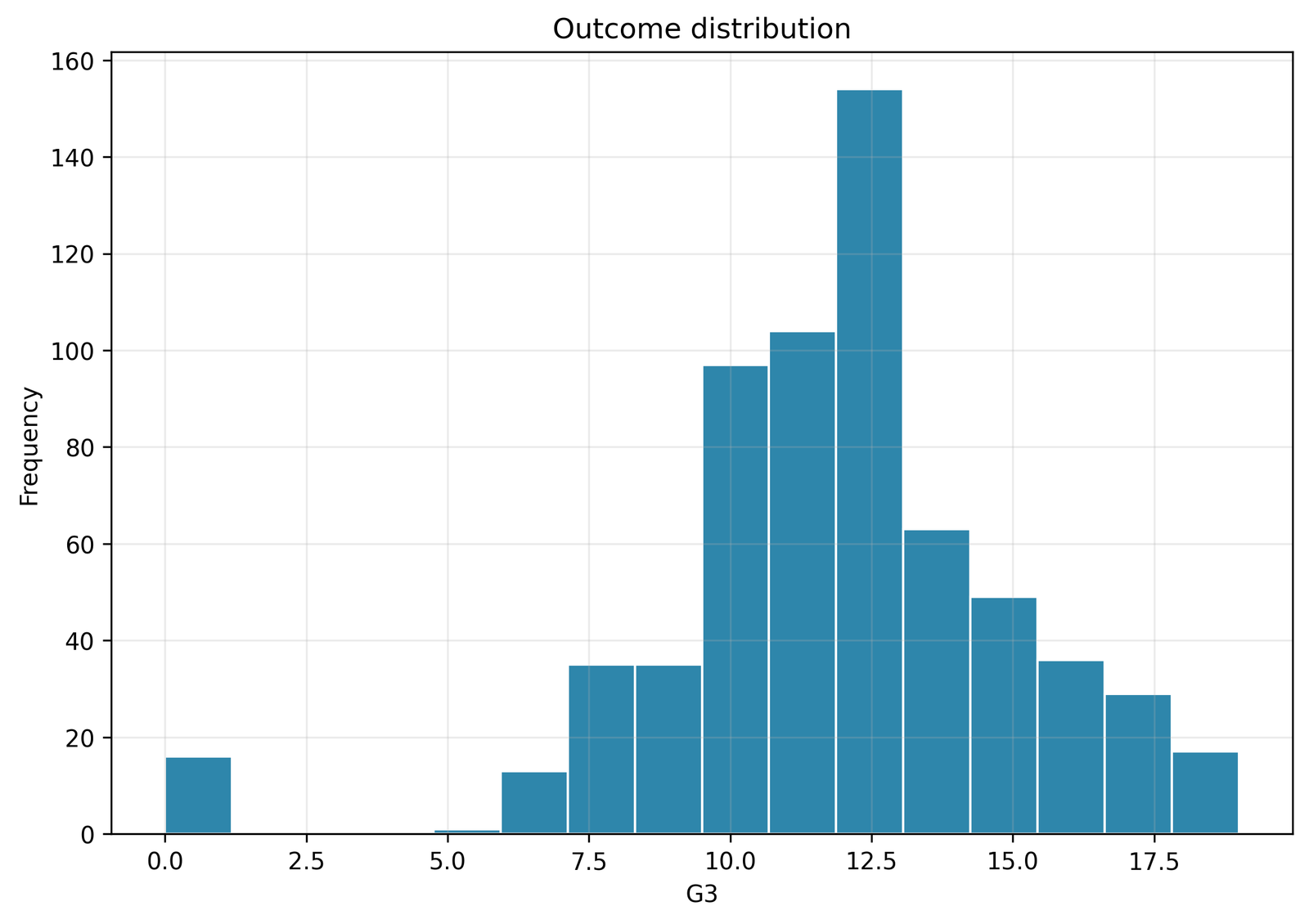
The outcome is concentrated in the middle grade range but includes low-end observations, including recorded zeros. The raw distribution supplies context, although Robust Regression weights are determined by conditional residuals rather than G3 alone.
The analysis contains 649 complete cases. The observed G3 range in the complete analysis data is 0 to 19.
An unusual outcome is not automatically influential. A case becomes strongly downweighted when its observed G3 differs greatly from the value predicted by G1, G2 and the other covariates.
The chart prevents the common mistake of defining outliers only from the marginal outcome distribution. Robust Regression evaluates disagreement with the fitted conditional relationship.
Python Chart 2: Observed G3 versus Huber Fitted Values
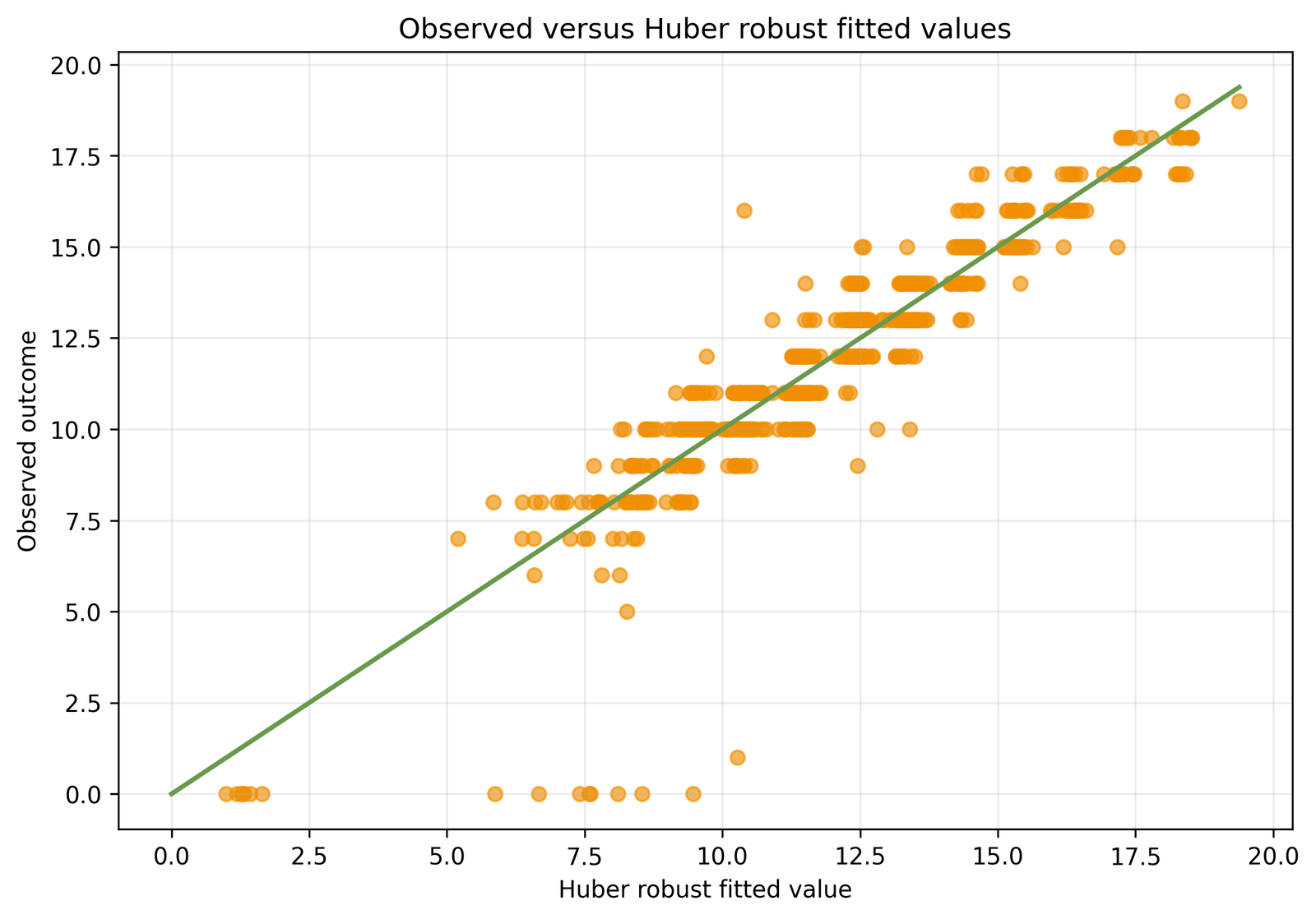
Most observations track the fitted relationship closely, while a small set has large vertical departures below the main cloud. Those departures generate the smallest Huber weights.
Case 164 has observed G3 = 0, OLS fitted = 9.0508 and Huber fitted = 9.4726. Case 173 has observed G3 = 1 with an OLS fitted value of 10.0330.
The fitted line captures the central grade pattern, but some recorded outcomes remain much lower than the model predicts. Robust Regression limits their coefficient influence without hiding them.
Overall alignment can coexist with important tail errors. The chart should be read with MAE, RMSE, residual plots and the low-weight case audit.
Python Chart 3: Huber Residuals versus Fitted Values

The main residual cloud is centered near zero, with visible grade-band structure and a negative tail. Robust weighting reduces coefficient pull but does not force the residual plot to become featureless.
The Python Huber scale is 0.7614459485. The minimum weight is 0.108117, 103 weights are below 0.80 and 24 are below 0.50.
Large negative residuals explain the strongest downweighting. Any curvature or changing spread would still indicate a mean-structure or variance problem that Huber Robust Regression alone does not solve.
Residual diagnostics remain necessary after robust fitting. Bounded influence is a protection mechanism, not proof that the linear specification is correct.
Python Chart 4: Huber Residual Normal Q-Q Plot
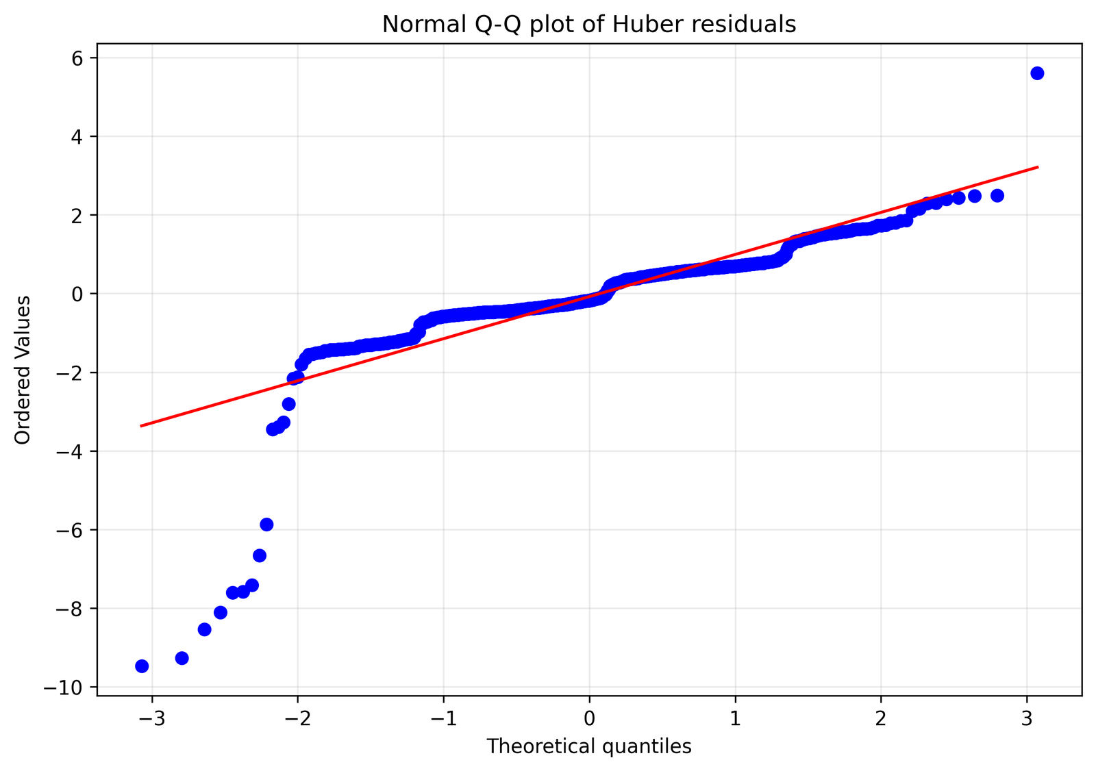
The middle of the distribution is closer to the reference line than the most extreme tails. Tail departures remain visible because Robust Regression changes coefficient influence rather than transforming the observed residuals into a normal distribution.
Huber uses c = 1.345 and scale 0.761446. Twenty-four cases receive less than half ordinary Huber weight.
The Q-Q pattern supports cautious large-sample inference and direct inspection of tail observations. It does not show that the low-weight cases are measurement errors.
Normality is not created by choosing a robust estimator. Prediction intervals and small-sample inference still require an appropriate distributional or resampling strategy.
Python Chart 5: OLS, Huber and Tukey Coefficient Comparison
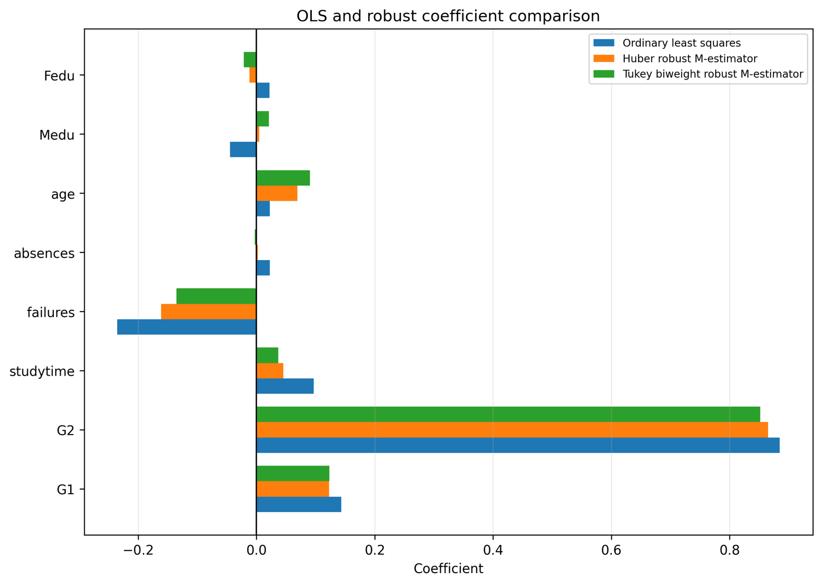
The strongest coefficients retain their direction across estimators, while smaller terms move more noticeably. G2 and failures are stable in direction; absences and parental-education terms are sensitive.
G2 changes from 0.8848 under OLS to 0.8650 under Huber. Absences changes from 0.0228 to 0.0022. Age changes from 0.0227 to 0.0693.
Coefficient movement identifies conclusions that depend on large-residual observations. Stability across estimators is stronger evidence than a single significance label.
The purpose of Robust Regression is not to select whichever coefficient looks preferable. The whole prespecified estimator must be interpreted and reported.
Python Chart 6: Huber Weights by Case
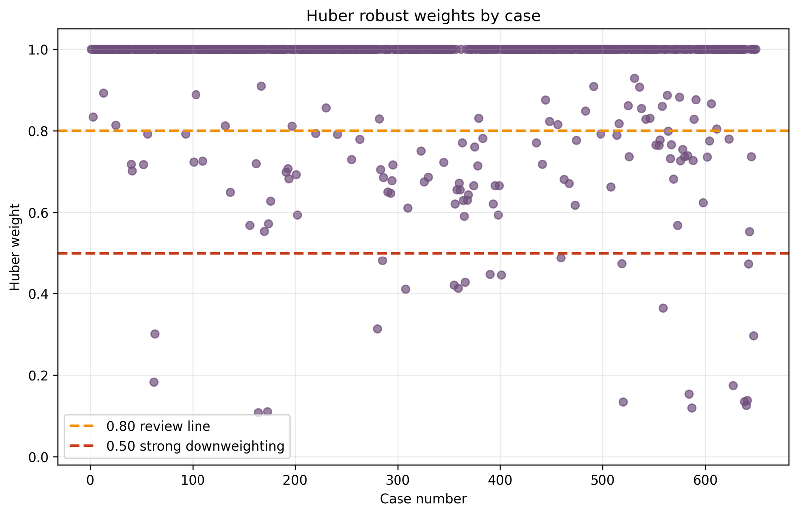
Most records sit at weight one, and a smaller group forms downward spikes. The lowest spikes correspond to cases whose observed outcomes conflict most strongly with the fitted linear equation.
The Huber median and first quartile are 1.0000, the mean is 0.9308, the minimum is 0.1081, 103 weights are below 0.80 and 24 are below 0.50.
Robust Regression is driven primarily by the majority pattern while retaining reduced contributions from extreme residuals. Weight is continuous, so there is no universal boundary between an ordinary and an invalid case.
The chart provides an auditable map for source verification. Any correction, exclusion or subgroup analysis should be documented separately and rerun from the original data.
R Charts and Paired Explanations
The R evidence independently cross-checks the Robust Regression calculations. The four unique R charts are arranged in two matched pairs, with a dedicated explanation beneath each chart.
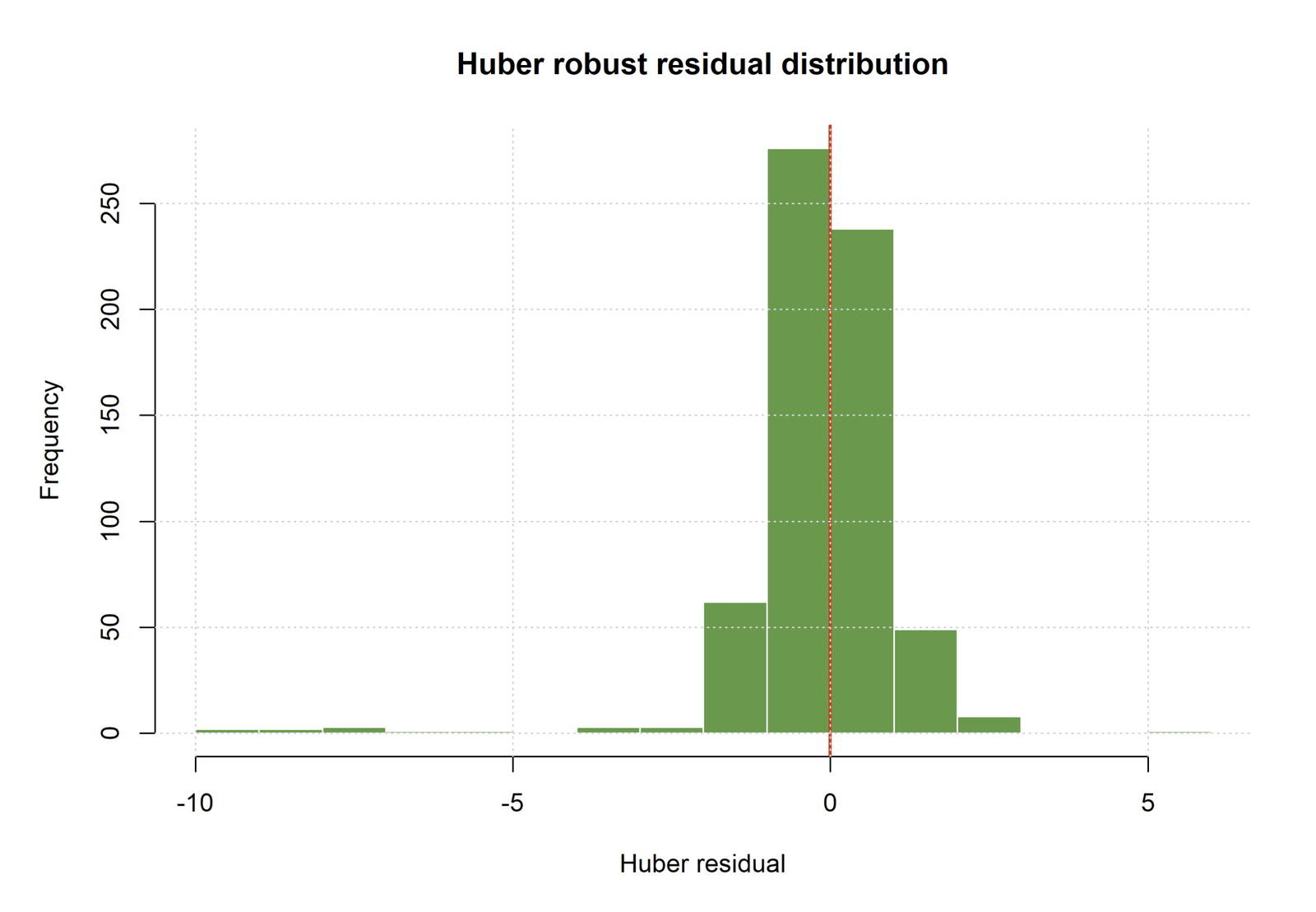
R Chart 1: Huber Residual Distribution
Pattern: The central mass is compact, while the negative tail contains observations that receive the strongest Huber downweighting.
Key values: R reports Huber scale 0.761631, close to the Python scale 0.761446.
Interpretation: The residual distribution explains why MAE can improve while RMSE increases: the robust fit prioritizes the central majority rather than minimizing the largest squared errors.
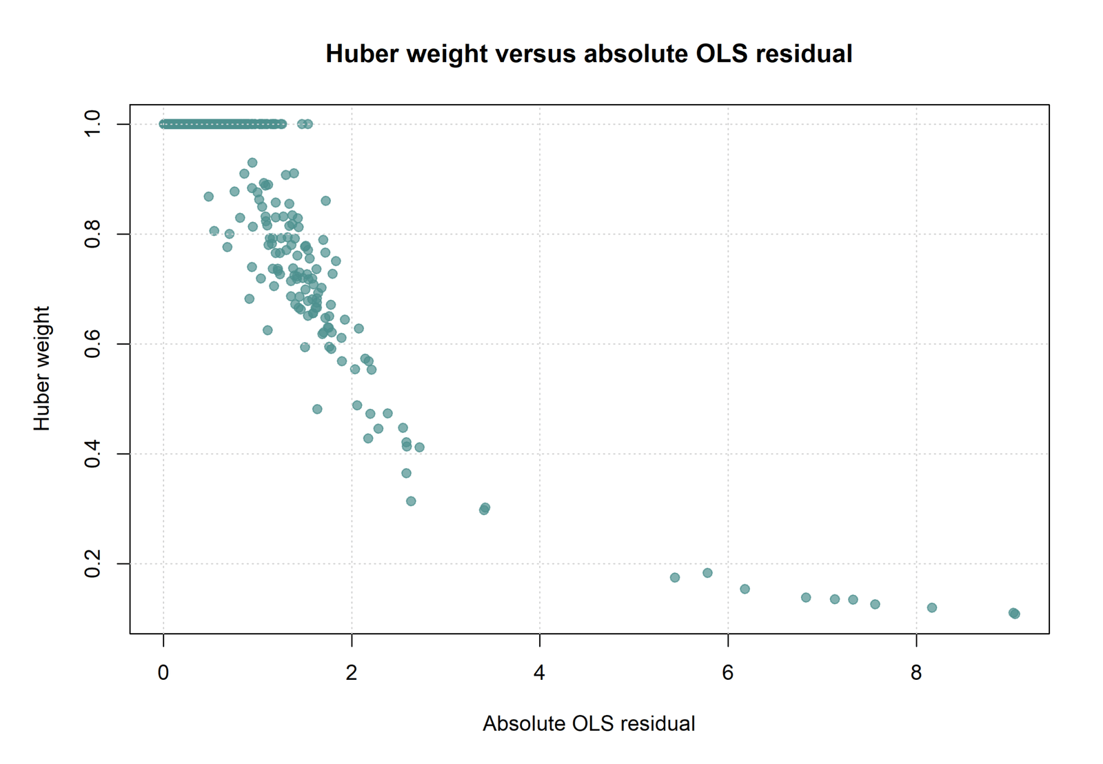
R Chart 2: Huber Weight versus OLS Residual
Pattern: Weights remain near one for ordinary residuals and decline as absolute residual magnitude increases.
Key values: The smallest Huber weight is approximately 0.108; 103 cases are below 0.80 and 24 are below 0.50.
Interpretation: The chart visualizes the bounded-influence rule. Direction alone does not determine weight; positive and negative residuals are downweighted according to magnitude after scale adjustment.
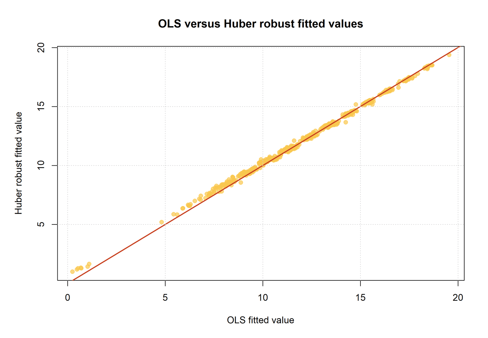
R Chart 3: OLS versus Huber Fitted Values
Pattern: Most fitted values are close because most observations retain full Huber weight. The largest differences occur where extreme residuals would otherwise pull the OLS equation.
Key values: OLS RMSE is 1.247020 and Huber RMSE is 1.262235 in the R cross-check; Huber MAE is 0.771730 versus 0.780019 for OLS.
Interpretation: Robust Regression produces a targeted adjustment rather than a completely different prediction surface.
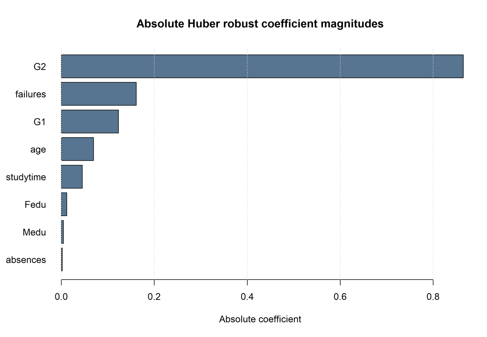
R Chart 4: Absolute Huber Coefficients
Pattern: G2 dominates the coefficient scale, G1 is the next clear positive slope, and the remaining estimates are much smaller in their original units.
Key values: Huber coefficients include G2 = 0.8650, G1 = 0.1228, failures = -0.1612 and age = 0.0693.
Interpretation: Absolute coefficient size is unit-dependent. The chart describes the fitted equation but does not prove causal importance or comparable standardized effects.
Robust Regression Coefficient and Parameter Interpretation
Primary Huber Equation
Each coefficient is a partial association under the fitted Huber Robust Regression model. For example, students differing by one point in G2 but equal on the other seven predictors differ by an estimated 0.8650 points in predicted G3. The interval [0.8214, 0.9085] shows that this positive association remains precise after residual downweighting.
G1 remains positive but decreases from 0.1434 to 0.1228. Failures remains negative and decreases in magnitude from -0.2354 to -0.1612. These changes indicate modest sensitivity rather than a reversal of the substantive direction.
Absences illustrates a fragile OLS conclusion. Its coefficient changes from 0.0228 under OLS to 0.0022 under Huber Robust Regression, and the Huber interval [-0.0117, 0.0160] contains zero. The data do not support treating the small positive OLS association as stable to large residuals.
Age becomes larger under Robust Regression, moving from 0.0227 to 0.0693, with interval [0.0139, 0.1247]. Downweighting can reveal a pattern that OLS extremes were suppressing; Robust Regression is not a shrinkage method that always moves coefficients toward zero.
Predictions, Effects and Model Meaning
A Huber Robust Regression prediction is obtained by substituting predictor values into the robust coefficient equation. For a hypothetical student with G1 = 10, G2 = 11, studytime = 2, failures = 0, absences = 4, age = 17, Medu = 3 and Fedu = 3, the fitted value is:
The value 11.3725 is a conditional point prediction on the G3 grade scale. It is not a probability and it is not automatically restricted to the observed grade range. The model should not be extrapolated to predictor combinations outside the analysis data without checking plausibility and validation performance.
Robust Regression weights are estimated from the observed residuals in the fitted sample. A new case does not arrive with a known robust weight before its outcome is observed. The prediction uses the robust coefficients; the historical weight distribution explains how the coefficients were estimated.
Robust Regression Assumptions and Diagnostics
Robust Regression still assumes that the selected linear predictor adequately represents the conditional center.
Independent observations are required unless clustering, repeated measures or time dependence are modeled.
Huber protects against vertical residual extremes but does not automatically neutralize high-leverage predictor patterns.
Convergence and Scale
The Python Huber Robust Regression fit converged in 33 iterations and estimated scale 0.7614459485. R reported scale 0.7616309207 and eight iterations. Different iteration counts do not indicate disagreement because software can use different starting values, scale updates and stopping tolerances. Final coefficients, fitted values and weight summaries provide the stronger validation target.
Residual Shape
Robust estimation does not remove residual skewness, heavy tails or heteroscedasticity. The residual-versus-fitted and Q-Q plots must still be inspected. The Q-Q Plot Normality Check is especially useful for separating central alignment from tail departures. Large-sample Huber inference is more resistant than conventional OLS to some departures, but dependence and variance misspecification still require attention.
High Leverage and Influence
A case can have an ordinary residual yet possess an unusual predictor combination. Such a case may influence the fitted slopes before residual downweighting becomes effective. Review leverage, Studentized Residuals and Cook’s Distance alongside the Robust Regression weights. A low Huber weight and high leverage answer different diagnostic questions.
Functional Form
A robust straight line is still a straight line. If the conditional mean is curved, an outlier-resistant linear estimator can downweight observations that are actually revealing misspecification. Inspect partial relationships, interactions and theory-guided nonlinear terms. The Nonlinear Regression guide explains when the mean function itself should change.
Weight Review
Case 164 has the minimum Huber weight of 0.108117. Its observed G3 is 0, the OLS fitted value is 9.050797 and the Huber fitted value is 9.472559. The observation remains in the Robust Regression model. Case 173 has observed G3 = 1 and OLS fitted = 10.0330, while case 587 has observed G3 = 0 and OLS fitted = 8.1676. These records deserve source review, not automatic deletion.
Robust Regression in Python, R, SPSS and Excel
Python
Python fits OLS, Huber and Tukey models on the same design matrix, exports coefficients, residuals and weights, and creates the six verified chart stories used above.
- Primary Huber tuning constant: 1.345
- Python Huber scale: 0.7614459485
- Python Huber iterations: 33
- Large-sample H1 covariance in the supplied workflow
R
R uses the same formula and rows to provide an independent Robust Regression cross-check through M-estimation.
- R Huber scale: 0.7616309207
- R iteration count: 8
- Minimum Huber weight: approximately 0.108148
- Four unique R charts with paired explanations
SPSS
The supplied SPSS PDF preserves a software-specific analysis path. Estimator, scale, tuning, leverage correction and covariance settings must be read from that output before numerical equivalence is claimed.
- Do not infer Huber c = 1.345 from a generic “robust” label.
- Keep the archived output with the reported article.
- Compare formulas and rows before comparing coefficients.
Excel
The worked workbook exposes model performance, coefficients, weight summaries, low-weight cases and side-by-side predictions.
- Visible Huber weight formula
- OLS and Huber prediction calculator
- Case-level audit with original values retained
- Educational verification rather than a hidden black-box fit
Code and Formula Panels
Python: OLS, Huber and Tukey Robust Regression
import statsmodels.api as sm

predictors = [
    "G1", "G2", "studytime", "failures",
    "absences", "age", "Medu", "Fedu"
]
X = sm.add_constant(data[predictors], has_constant="add")
y = data["G3"]

ols = sm.OLS(y, X).fit()
huber = sm.RLM(
    y,
    X,
    M=sm.robust.norms.HuberT(t=1.345)
).fit(maxiter=200, cov="H1")

tukey = sm.RLM(
    y,
    X,
    M=sm.robust.norms.TukeyBiweight()
).fit(maxiter=200, cov="H1")

case_audit = data.copy()
case_audit["ols_fitted"] = ols.fittedvalues
case_audit["huber_fitted"] = huber.fittedvalues
case_audit["huber_residual"] = y - huber.fittedvalues
case_audit["huber_weight"] = huber.weights
case_audit["tukey_weight"] = tukey.weights
Use stable case identifiers before sorting the audit. The same rows and predictor order must be retained for all three Robust Regression comparisons.
R: MASS robust linear models
form <- G3 ~ G1 + G2 + studytime + failures +
  absences + age + Medu + Fedu

ols <- lm(form, data = dat)

huber <- MASS::rlm(
  form,
  data = dat,
  psi = MASS::psi.huber,
  k2 = 1.345,
  method = "M",
  maxit = 200
)

tukey <- MASS::rlm(
  form,
  data = dat,
  psi = MASS::psi.bisquare,
  method = "M",
  maxit = 200
)

huber_weights <- huber$w
huber_fitted <- fitted(huber)
huber_residuals <- resid(huber)
R and Python can use different scale and convergence mechanics. Reconcile final Robust Regression estimates rather than forcing iteration counts to match.
Excel: Huber weight and prediction formulas
Standardized residual:
=([@Observed]-[@Huber_Fitted])/$B$2

Huber weight with c in B3:
=IF(ABS([@Std_Residual])<=$B$3,1,$B$3/ABS([@Std_Residual]))

Huber fitted value:
=$B$6+$B$7*[@G1]+$B$8*[@G2]+$B$9*[@studytime]
+$B$10*[@failures]+$B$11*[@absences]+$B$12*[@age]
+$B$13*[@Medu]+$B$14*[@Fedu]
The workbook formulas audit a converged Robust Regression solution. A spreadsheet becomes a full IRLS estimator only when scale, weights and coefficients are updated repeatedly to convergence.
SPSS: verification checklist for the supplied output
- Confirm the dependent variable is G3 and the predictor list contains the same eight fields.
- Identify the exact robust estimator, tuning constant and scale definition in the output.
- Confirm whether reported uncertainty is bootstrap, sandwich, normal approximation or another method.
- Save fitted values, residuals and case weights when the procedure supports them.
- Do not label an SPSS result equivalent to Huber c = 1.345 unless the output documents matching settings.
Advanced Robust Regression Topics
These 26 panels extend the worked analysis from computation to estimator choice, diagnostics, prediction, inference and responsible case review.
1. Robust Regression Estimand and Research Question
Robust Regression estimates the coefficient vector solving a bounded-influence estimating equation for the selected conditional mean. The target is not “the model after outliers are removed.” It is the linear relationship defined by a particular loss, scale rule and tuning constant.
State whether the objective is resistant estimation, coefficient sensitivity, central prediction or protection from heavy-tailed errors. A clear estimand prevents the Huber result from being treated as a convenient alternative only when OLS is inconvenient.
2. Huber Influence Function in Robust Regression
The Huber score is linear near zero and capped in magnitude outside the tuning threshold. This gives Robust Regression bounded residual influence while retaining a smooth, convex objective. Convexity makes the solution computationally stable and avoids the multiple-local-minimum behavior associated with some redescending losses.
The cap applies after residuals are divided by the robust scale. Therefore, the same raw residual may receive a different weight in a dataset with a different error scale.
3. Iteratively Reweighted Least Squares Mechanics
IRLS converts the nonlinear Robust Regression estimating equation into a sequence of weighted least-squares problems. At iteration k, the current coefficients generate residuals, residuals generate weights and weights generate the next coefficient vector.
Convergence means the numerical updates stabilized under the software tolerance. It does not prove that the predictors are correctly specified, that the sample is representative or that the residual distribution is harmless.
4. Robust Scale Estimation
The scale parameter controls which residuals are considered ordinary relative to the tuning constant. A scale estimate that is inflated by extremes would weaken downweighting, while a scale estimate that is too small would downweight too many observations.
The Python and R scale estimates, 0.761446 and 0.761631, are very close. This agreement supports the computational stability of the worked Robust Regression solution.
5. Why Huber c = 1.345 Is Reported
The tuning constant determines the transition from quadratic to linear loss. A smaller c produces stronger resistance and lower Gaussian efficiency; a larger c makes Robust Regression increasingly similar to OLS.
The value 1.345 is a conventional efficiency-resistance compromise. It is still an analysis setting that must be reported. Changing c after examining preferred coefficients would be an outcome-driven sensitivity decision.
6. Tukey Biweight Robust Regression
Tukey biweight is redescending, so the score returns toward zero for sufficiently extreme standardized residuals. In the worked data, the minimum Tukey weight is zero and 128 cases receive weights below 0.80.
Tukey slightly lowers MAE and median absolute error relative to Huber while increasing RMSE. That pattern is consistent with a stronger focus on the central majority. The entire Tukey model should be reported as sensitivity evidence, not mined coefficient by coefficient.
7. Efficiency versus Resistance
OLS is highly efficient when the Gaussian linear model is well specified. Robust Regression deliberately gives up some ideal-model efficiency to reduce the effect of tail observations. The small RMSE increase from 1.2470 to 1.2622 reflects that trade-off in the worked sample.
The slightly lower Huber MAE and median absolute error show improved typical absolute fit. Neither result establishes a universal winner because the loss function defines what “best” means.
8. Breakdown Point and Robust Regression
Bounded influence and breakdown point are related but different robustness concepts. Huber M-estimation bounds the effect of large residuals at fixed predictor positions, but classical M-estimation can still be vulnerable to high-leverage contamination in predictor space.
A high-breakdown estimator may resist a larger fraction of contaminated cases, but it may use different algorithms and have different efficiency. Do not claim a high breakdown point for the present Huber Robust Regression fit without a matching estimator specification.
9. Vertical Outliers versus High Leverage
A vertical outlier has a large outcome residual for its predictor values. A high-leverage case has an unusual predictor combination. Huber Robust Regression directly limits the first type through residual weights but may not fully protect against the second type.
Review leverage and influence diagnostics alongside weights. A high-leverage observation can pull the fitted line toward itself and then display a modest residual, thereby escaping strong residual downweighting.
10. Masking and Swamping
Masking occurs when several unusual observations support one another and reduce their apparent residuals. Swamping occurs when ordinary cases look unusual because the fitted model has been distorted. Robust Regression can reduce these effects, but it cannot guarantee their absence.
Compare case weights, leverage, residual patterns and sensitivity refits. Clusters of low weights sharing a subgroup or predictor pattern often indicate missing structure rather than isolated bad records.
11. Continuous Robust Regression Weights
A weight of 0.49 is not categorically different from 0.51. Thresholds such as 0.80 or 0.50 summarize the distribution and direct review; they do not define valid versus invalid observations.
The worked Huber Robust Regression model has 103 weights below 0.80 and 24 below 0.50. Reporting the full distribution is more informative than naming only the most extreme case.
12. Coefficient Stability Analysis
Coefficient stability compares the same term across OLS, Huber and Tukey models fitted to the same rows and design. G2 is highly stable, while absences, age and parental education are more sensitive.
Stability should be interpreted in magnitude, direction and uncertainty. A coefficient can retain its sign but change enough to alter substantive meaning, or move away from zero when influential cases had masked the broader relationship.
13. Robust Regression Confidence Intervals
The supplied Huber intervals use a large-sample normal approximation. They are not finite-sample OLS t intervals and should be labeled accordingly. With 649 observations, asymptotic inference may be useful, but dependence, leverage and misspecification remain relevant.
Bootstrap inference can be considered when the resampling design reflects the sampling structure. For clustered data, resample clusters rather than individual rows.
14. Heteroscedasticity and Robust Regression
Huber Robust Regression limits residual influence but does not automatically model nonconstant conditional variance. Heteroscedasticity can still affect uncertainty and prediction intervals.
Distinguish robust coefficients from robust covariance. A sandwich covariance changes uncertainty for a fitted estimator, while Huber changes the estimating equation and therefore the point estimates. Both may be needed when residual tails and heteroscedasticity coexist.
15. Nonlinearity in Robust Regression
When the mean relationship is curved, a robust linear model can mistake systematic curvature for outlying residuals. Downweighting those observations may conceal rather than solve the misspecification.
Inspect residual-versus-fitted patterns and theory-guided partial relationships. Add transformations, splines or interactions before interpreting low weights as isolated anomalies.
16. Categorical Predictors and Interactions
Robust Regression can include dummy-coded categorical predictors and interaction terms. Interpretation depends on the reference category and coding, just as in OLS. The robust loss changes case influence, not the meaning of the design matrix.
When a subgroup receives many low weights, investigate whether an omitted interaction or group-specific slope is needed. A single pooled robust line may be inadequate even if its overall residual resistance is strong.
17. Missing Data and the Analysis Sample
The worked Robust Regression analysis uses 649 complete records. Complete-case fitting is transparent but assumes that excluding incomplete rows does not create serious selection bias under the intended interpretation.
Imputation, if used, should be performed before model fitting and should preserve the uncertainty and sampling structure. Robust weighting is not a missing-data method.
18. Cross-Validation for Robust Regression
In-sample RMSE, MAE and median absolute error describe the fitted sample. Future prediction should be evaluated with cross-validation or a held-out test set. Each fold must fit OLS and Robust Regression only on its training partition.
Do not calculate robust weights on the full dataset and reuse them inside validation folds. That would leak outcome information from the assessment cases into model training.
19. Prediction and Extrapolation
Robust Regression changes the coefficient surface but does not automatically produce robust prediction intervals. A new case can be far outside the predictor range even when its point prediction is numerically plausible.
Inspect predictor support, leverage and calibration. Extrapolation remains risky because bounded residual influence in the training sample cannot create information where the data contain none.
20. Robust Standard Errors versus Robust Regression
“Robust regression” and “robust standard errors” should not be used interchangeably. Heteroscedasticity-consistent standard errors keep the OLS coefficients unchanged. Huber Robust Regression changes the coefficients by changing observation influence.
A report should state both the estimator and the covariance method. Saying only “robust results were used” is not reproducible.
21. Quantile Regression Comparison
Quantile regression estimates a conditional median or another quantile, whereas Huber Robust Regression estimates a bounded-influence conditional center defined by its score equation. The two methods can produce different coefficients because they answer different questions.
Use quantile regression when the research target is a conditional quantile or when effects across the outcome distribution are substantively important. Use Huber when resistance of a linear center estimate is the primary aim.
22. Student-t Regression Comparison
A Student-t regression model specifies a heavy-tailed probability distribution and estimates a likelihood. Huber Robust Regression does not require that full tail distribution; it uses a bounded score.
The Student-t approach can provide coherent likelihood-based intervals and predictions when its distribution is appropriate. Huber offers simpler resistance but requires careful asymptotic or resampling inference.
23. Weighted Least Squares Comparison
Weighted least squares assigns weights intended to represent precision or inverse variance. Huber Robust Regression weights are generated from residual disagreement with the current fitted model.
Using Huber weights as if they were known sampling precisions would misinterpret their purpose. Conversely, replacing known design or survey weights with robust weights would change the estimand.
24. Data Correction, Trimming and Winsorizing
Data correction requires evidence from the source record. Trimming removes observations and winsorizing changes observed values. Robust Regression does neither; it retains the original data and reduces score influence through the estimator.
Any corrected or excluded analysis should be versioned and presented beside the original. Never select a deletion because it creates a desired significance result.
25. Python, R, SPSS and Excel Reproducibility
Reproducible Robust Regression requires the exact formula, rows, intercept convention, loss, tuning constant, scale rule, covariance method and stopping settings. Iteration counts can differ while final estimates agree closely.
The verified Python and R scales differ only slightly. The SPSS PDF and Excel workbook provide separate audit paths, but they should not be declared numerically equivalent without matching settings.
26. Robust Regression Decision Framework
Begin with the research question and a defensible mean structure. Fit OLS as a transparent baseline, diagnose residual and leverage behavior, fit a prespecified Huber Robust Regression model, and use Tukey or another estimator as a whole-model sensitivity analysis.
Report stable and sensitive coefficients, the weight distribution, in-sample metrics, limitations and case-review policy. The defensible conclusion is about sensitivity of the fitted relationship, not about whether unusual observations are “good” or “bad.”
APA-Style Reporting
Worked Robust Regression Report
A Huber M-estimator predicted final grade G3 from G1, G2, studytime, failures, absences, age, maternal education and paternal education in 649 complete records. The Huber tuning constant was 1.345. The Python Robust Regression model converged in 33 iterations and estimated a residual scale of 0.7614. The minimum Huber weight was 0.1081; 103 observations received weights below 0.80 and 24 received weights below 0.50.
Huber RMSE was 1.2622, MAE was 0.7717 and median absolute error was 0.5136, compared with OLS values of 1.2470, 0.7800 and 0.5422, respectively. G2 remained positively associated with G3, b = 0.8650, 95% CI [0.8214, 0.9085], while failures remained negatively associated, b = -0.1612, 95% CI [-0.2819, -0.0404]. The absences coefficient decreased from 0.0228 under OLS to 0.0022 under Huber Robust Regression, indicating sensitivity to large-residual observations. Huber intervals used a large-sample normal approximation. A Tukey biweight model was retained as a stronger whole-model sensitivity analysis. Low-weight cases were not automatically deleted.
A complete Robust Regression report should name the loss function, tuning constant, scale convention, covariance approximation, sample, formula, convergence outcome, weight distribution, coefficient comparison, prediction metrics and policy for reviewing low-weight cases.
Publication Checklist
- Confirm OLS, Huber and Tukey use the same 649 rows and eight predictors.
- Archive the exact coding for G3, G1, G2, studytime, failures, absences, age, Medu and Fedu.
- State that Huber Robust Regression uses c = 1.345.
- Record the scale convention and software-specific convergence information.
- Export OLS, Huber and Tukey coefficients in one comparison table.
- Report RMSE, MAE and median absolute error without declaring one universal winner.
- Preserve Huber and Tukey weights with stable case identifiers.
- Investigate low-weight records against source evidence before any correction.
- Inspect residual shape, leverage, heteroscedasticity and functional form.
- Label Huber intervals as large-sample normal approximations.
- Keep Python, R, SPSS and Excel results tied to their exact settings.
- Validate predictive claims with resampling or an external sample.
- Report sensitive coefficients rather than saying the robust model simply confirms OLS.
- Version any changed data value, exclusion or alternate tuning constant.
- Keep the original outputs available for audit.
- Use only the confirmed Robust Regression downloads and chart assets.
Downloads and Verification Resources
Quick PDF Downloads
Use the software report that matches the analysis you need to reproduce.
Frequently Asked Questions
What is Robust Regression?
Robust Regression is a family of estimators that limits the effect of unusually large residuals. The worked analysis uses Huber M-estimation as primary and Tukey biweight as a stronger sensitivity model.
When should Robust Regression be used?
Use Robust Regression when a continuous-outcome linear model is substantively appropriate but coefficients may be sensitive to vertical outliers or heavy-tailed residuals. It does not replace checking leverage, nonlinearity or sampling dependence.
How many records were analyzed?
All 649 complete records were used in OLS, Huber Robust Regression and Tukey Robust Regression with the same eight predictors.
What is the Huber tuning constant?
The primary Robust Regression fit uses c = 1.345. It determines where the loss changes from quadratic to linear.
Does Huber Robust Regression delete outliers?
No. It retains every observation and lowers the estimating weight of cases with large standardized residuals.
What was the minimum Huber weight?
Python reported a minimum Robust Regression weight of 0.108117. R reported approximately 0.108148, which is a close cross-software agreement.
How many cases were materially downweighted?
A total of 103 Huber weights were below 0.80 and 24 were below 0.50. These are review counts, not deletion counts.
Did Robust Regression improve RMSE?
No. OLS RMSE was 1.247020 and Huber RMSE was 1.262243. OLS is optimized for squared error on the fitted sample.
Did Robust Regression improve absolute-error metrics?
Slightly. Huber MAE decreased from 0.780019 to 0.771728, and median absolute error decreased from 0.542167 to 0.513587.
Which coefficient was most stable?
G2 was the clearest stable Robust Regression result: 0.8848 under OLS and 0.8650 under Huber.
Which coefficient was most sensitive?
Absences changed from 0.0228 under OLS to 0.0022 under Huber Robust Regression, and the Huber interval included zero.
What is Tukey biweight?
Tukey biweight is a redescending Robust Regression estimator that can assign zero weight to sufficiently extreme standardized residuals. It is used here as a stronger whole-model sensitivity check.
Are Huber p-values exact small-sample tests?
No. The supplied Robust Regression intervals and p-values use a large-sample normal approximation.
Does Robust Regression solve high leverage?
Not completely. A predictor-space extreme can influence slopes even with a modest residual, so leverage and Cook’s distance remain important.
Why do Python and R show different iteration counts?
Robust Regression implementations can use different starting values, scale updates and stopping tolerances. Final coefficients, fitted values and weight distributions are the meaningful cross-check.
Is Robust Regression causal?
No. Robust Regression limits residual influence but does not remove confounding, selection bias, measurement error or other barriers to causal interpretation.
Robust Regression Conclusion
The verified Huber Robust Regression model retains all 649 observations while reducing the contribution of large residuals. The minimum Huber weight is 0.1081, 103 weights are below 0.80 and 24 are below 0.50. G2 remains strongly positive and failures remains negative, while absences, age and the parental-education coefficients show greater sensitivity to the influence function.
Huber Robust Regression slightly lowers MAE and median absolute error but slightly increases RMSE relative to OLS. That trade-off is expected because the estimator protects the central relationship rather than minimizing the largest squared errors. Tukey biweight confirms that stronger downweighting produces a similar central story while moving some sensitive terms further.
The defensible conclusion is not that Robust Regression discovers “bad” cases. It provides a transparent sensitivity-resistant estimate, an auditable weight for every record and a principled way to distinguish stable from fragile coefficients. Correct use requires the same care as any regression analysis: a justified mean structure, leverage and residual diagnostics, appropriate inference, validation, source verification and honest reporting of all estimator settings.

