
Regression in SPSS: Dialog Steps, Syntax, Output Tables, Diagnostics and Interpretation
Regression in SPSS is presented here as a complete SPSS-only workflow. The article follows the verified 649-case output from data screening and correlations through simple and multiple REGRESSION procedures, Model Summary, ANOVA, coefficients, collinearity diagnostics, casewise output, saved residual variables, three SPSS charts and the 95-page Viewer export.
2 ENTER procedures
8 saved multiple-model diagnostics
95-page Viewer export
Regression in SPSS Model Overview
Regression in SPSS estimates a continuous dependent variable from one or more independent variables. The verified simple procedure predicts final grade G3 from G2. The verified multiple procedure predicts G3 from G1, G2, studytime, failures, absences, age, Medu and Fedu, with all eight predictors entered simultaneously through METHOD=ENTER.
Both procedures use 649 valid cases. The simple procedure reports R² = .844 and standard error of the estimate = 1.27810. The multiple procedure reports R² = .851, adjusted R² = .849, standard error = 1.25576 and Durbin-Watson = 1.862. The increase in fitted performance is modest because G2 alone already carries most of the grade-history signal.
What Is Regression in SPSS?
Regression in SPSS uses ordinary least squares in the Linear Regression procedure. The unstandardized B coefficients reconstruct the fitted equation. Standardized Beta values support within-model scale comparison. The Model Summary describes fit, the ANOVA table tests the complete predictor block, and the Coefficients table tests individual conditional slopes.
When Should Regression in SPSS Be Used?
Good uses
- Estimating a continuous outcome with a prespecified predictor set.
- Producing standard Model Summary, ANOVA and Coefficients tables.
- Saving predictions and residual diagnostics to the active dataset.
- Reviewing tolerance, VIF, condition indices and casewise diagnostics.
- Preserving an auditable SPV and stable PDF output record.
Weak uses
- Applying linear regression to an outcome requiring another model family.
- Relying on menu memory without saving syntax.
- Calling a conditional slope a causal effect without design support.
- Calling fitted standard error future prediction accuracy.
- Deleting predictors or cases automatically from one diagnostic threshold.
Core Assumptions and Requirements
1. Continuous dependent variable and correct model family
G3 is treated as a continuous dependent variable. Binary, count, ordinal, censored and survival outcomes require procedures whose scale and distribution match those outcomes.
2. Correct active dataset and case population
The Notes tables should identify the expected active dataset, 649 cases, no unintended filter, no weighting and no Split File groups.
3. Linear conditional mean
The expected value of G3 should be adequately represented by the additive predictor equation. Residual-versus-predicted evidence is used to review curvature.
4. Independent observations
Independence comes from the design and observation structure. Durbin-Watson is meaningful only when case order represents a substantive sequence.
5. Reasonably stable residual variance
The residual plot should be reviewed for changing vertical spread. Strong fitted R² does not guarantee homoscedasticity.
6. No exact predictor dependence
Tolerance, VIF and collinearity diagnostics assess predictor overlap. G1 and G2 overlap substantially but are not exact duplicates.
7. Reproducible syntax and saved output
The syntax, source data state, augmented SAV, SPV and PDF should be archived together so every reported table can be reproduced.
Quick Answer
Regression in SPSS supports a strong fitted relationship for G3. G2 is the dominant adjusted predictor, G1 adds a smaller positive coefficient, failures has a negative conditional coefficient and absences has a small positive adjusted coefficient. Casewise and residual evidence still matters despite the high R².
What the verified Viewer supports
- 649 valid cases are used in the regression procedures.
- The eight-predictor ENTER block is statistically significant.
- The multiple model explains approximately 85.1% of fitted G3 variation.
- G2 has B = .885 and standardized Beta = .798.
- G1, G2, failures and absences have displayed intervals excluding zero.
- Predicted, residual, leverage and influence variables were saved.
What the Viewer does not prove
- It does not establish causal effects.
- It does not guarantee the same accuracy in future cohorts.
- It does not show that every predictor contributes meaningfully.
- It does not make Sig. .000 equal to a probability of zero.
- It does not justify automatic removal of case 164 or any flagged case.
- It does not make stale setup pages part of the valid statistical evidence.
Table of Contents
- Why this analysis needs Regression in SPSS
- How Regression in SPSS works
- Viewer provenance and page map
- Variables, coding and saved diagnostics
- SPSS dialog steps
- Regression in SPSS results
- SPSS charts and explanations
- Coefficient interpretation
- Predictions and model meaning
- Assumptions and diagnostics
- SPSS workflow and reproducibility
- Corrected SPSS syntax
- Advanced Regression in SPSS topics
- APA-style reporting
- Publication checklist
- Downloads and chart resources
- Related Salar Cafe guides
- Frequently asked questions
- Regression in SPSS conclusion
Why This Analysis Needs Regression in SPSS
Regression in SPSS is appropriate because the research question concerns a continuous final grade and a prespecified block of explanatory variables. The ENTER method keeps the complete adjustment set fixed instead of choosing predictors from sample significance.
The simple model answers a bivariate question: how does expected G3 differ with G2? The multiple model asks how expected G3 differs with each predictor while the remaining seven predictors are held constant. These are different statistical questions even when their tables appear in the same Viewer file.
Regression in SPSS also provides a useful teaching record. The Variables Entered/Removed table confirms METHOD=ENTER, the Model Summary reports fitted strength, ANOVA tests the full block, the Coefficients table shows B and Beta, and saved residual variables connect the output with charts and individual cases.
How Regression in SPSS Works
Regression in SPSS follows three linked stages: prepare the active dataset, run the declared ENTER procedures, and interpret the Viewer together with the saved diagnostic variables.
Check variable types, missing definitions, filters, weights, Split File and 649 valid cases.
Fit G3 on G2, then fit G3 on the fixed eight-predictor block.
Reconcile fit, ANOVA, coefficients, collinearity, residuals, cases and charts.
METHOD=ENTER
METHOD=ENTER enters all listed predictors simultaneously. It is not forward, backward or stepwise selection. The multiple coefficient for G2 is therefore adjusted for G1, studytime, failures, absences, age, Medu and Fedu.
The Variables Entered/Removed table should list the same eight names as the syntax. If a variable is omitted, renamed or excluded through a missing-value problem, the interpretation changes even if the Model Summary still looks plausible.
Ordinary Least Squares
The procedure estimates coefficients that minimize the sum of squared residuals. SPSS reports the fitted equation through the unstandardized B column. The standardized Beta column is supplementary and should never replace B in a prediction equation.
Simple and Multiple Procedures
The simple procedure has one predictor and 647 residual degrees of freedom. The multiple procedure has eight predictors and 640 residual degrees of freedom. Both use 649 cases, so their displayed fit values can be compared without a changing-case-count problem.
The simple standard error is 1.27810 and the multiple standard error is 1.25576. The small reduction shows that the additional predictors improve fitted description, but G2 already provides an exceptionally strong baseline.
Why Table Reconciliation Matters
A defensible Regression in SPSS result should satisfy several identities. Total degrees of freedom should equal 648. Regression and residual sums of squares should add to total sum of squares. The coefficient rows should match the Variables Entered table. Saved predictions should recreate the equation, and saved residuals should equal observed minus predicted.
SPSS Viewer Provenance and Page Map
Regression in SPSS is supported by a 95-page exported Viewer record. The opening setup pages are not uniform in provenance: pages 1 through 7 contain stale HOST notes from an earlier folder state. They are disclosed and excluded from statistical interpretation. The applicable regression record begins with the correct import section around page 9 and later Notes tables identify the correct active dataset and 649 cases.
Why SPV and PDF Serve Different Purposes
The SPV preserves editable native tables, Notes and chart objects. The PDF provides a stable review copy but can split wide tables across pages and retain stale pages from an earlier output state. The syntax determines the procedure; the SPV preserves native output; the PDF supports distribution and page-level auditing.
How to Audit a Long Viewer File
- Read the Notes table for active dataset, filter, weight, Split File and cases.
- Confirm the procedure title and dependent variable.
- Confirm METHOD=ENTER and the predictor list.
- Read Model Summary and ANOVA together.
- Follow Coefficients table continuations before recording intervals, correlations or VIF.
- Match saved-variable names with the diagnostics section.
- Trace charts to their command and page number.
- Exclude stale or unrelated setup pages explicitly rather than silently.
Variables, Coding and Saved Diagnostics
Regression in SPSS depends on the Variable View definitions and the active case settings. All nine analysis variables are numeric in the verified procedure, with G3 as the dependent variable and the remaining columns used as predictors.
| Variable | Role | Substantive label | SPSS review |
|---|---|---|---|
| G3 | Dependent | Final grade outcome. | Scale variable; observed value used in residual calculations. |
| G2 | Simple and multiple predictor | Second-period grade. | Scale predictor; strongest fitted Beta. |
| G1 | Multiple predictor | First-period grade. | Scale predictor with substantial G2 overlap. |
| studytime | Multiple predictor | Weekly study-time predictor. | Entered as a numeric linear term. |
| failures | Multiple predictor | Past class failures. | Numeric count with negative adjusted B. |
| absences | Multiple predictor | School absences. | Numeric count with small positive adjusted B. |
| age | Multiple predictor | Student age. | Scale predictor; displayed interval includes zero. |
| Medu | Multiple predictor | Mother education. | Ordered code entered as a numeric linear term. |
| Fedu | Multiple predictor | Father education. | Ordered code entered as a numeric linear term. |
Descriptive Anchors
All nine variables have 649 valid cases and zero missing cases in the verified output. G3 has mean 11.9060 and standard deviation 3.23066. G2 has mean 11.5701 and standard deviation 2.91364. Complete columns make pairwise and listwise counts agree here, but the missing-data method should still be documented.
The correlation table reports G3 correlations of .919 with G2, .826 with G1, −.393 with failures and −.091 with absences. These are zero-order relationships and must not be substituted for the adjusted B coefficients.
Saved Simple-Model Variables
| Saved name | Meaning | Use |
|---|---|---|
| simple_pred | Unstandardized predicted G3. | Observed-versus-predicted and residual calculations. |
| simple_resid | Unstandardized residual. | Raw case error on the grade scale. |
| simple_zpred | Standardized predicted value. | Scale-free diagnostic plotting. |
| simple_zresid | Standardized residual. | Screening unusual simple-model errors. |
Saved Multiple-Model Variables
| Saved name | Meaning | Use |
|---|---|---|
| multi_pred | Unstandardized predicted G3. | Prediction comparison and case equation audit. |
| multi_resid | Unstandardized residual. | Raw error and residual distribution. |
| multi_zpred | Standardized predicted value. | Standardized diagnostic scale. |
| multi_zresid | Standardized residual. | Casewise threshold review. |
| multi_sresid | Studentized residual. | Residual scaled using case-sensitive variance. |
| multi_mahal | Mahalanobis distance. | Unusual multivariable predictor profiles. |
| multi_cook | Cook’s distance. | Combined residual and leverage influence. |
| multi_lev | Centered leverage value. | Unusual position in predictor space. |
Regression in SPSS Dialog Steps
Regression in SPSS can be configured through Analyze → Regression → Linear, but the final syntax should always be saved. The dialog steps below correspond to the verified multiple procedure.
Step 1: Open Linear Regression
Choose Analyze → Regression → Linear. Move G3 into the Dependent box. Move G1, G2, studytime, failures, absences, age, Medu and Fedu into the Independent(s) box. Select Enter as the method.
Step 2: Request Statistics
Open Statistics and request Estimates, Model fit, R squared change, Descriptives, Part and partial correlations, Collinearity diagnostics, Confidence intervals at 95% and Durbin-Watson. The exact available wording can vary by SPSS version, but the resulting syntax should include the corresponding /STATISTICS and /RESIDUALS DURBIN options.
Step 3: Request Casewise Output
Request casewise diagnostics for standardized residuals greater than three in absolute value. This produces a casewise table for unusually large errors. The threshold is a screening rule, not a deletion rule.
Step 4: Save Diagnostic Variables
Open Save. Request unstandardized predicted values, unstandardized residuals, standardized predicted values, standardized residuals, studentized residuals, Cook’s distance, leverage and Mahalanobis distance. The syntax names these variables explicitly so they remain identifiable after the procedure.
Step 5: Review Plots
The native REGRESSION dialog can request standardized residual plots, but the verified workflow also creates explicit graphs from the named saved variables. This makes the exact pairing visible: G3 with multi_pred, multi_resid with multi_pred, and a histogram of multi_resid.
Step 6: Paste Rather Than Click OK
Choose Paste to send the command to the Syntax Editor. Review the dependent variable, method, predictor order, confidence interval, collinearity, casewise, residual and save settings. Then execute the syntax and archive it with the output.
Regression in SPSS Results
Regression in SPSS produces a strong simple model and a slightly stronger eight-predictor model. The valid tables below are reconstructed from the applicable Viewer record.
Valid in both procedures
G3 on G2
Eight-predictor ENTER
Multiple procedure
Multiple residual scale
Eight and 640 df
Verified Model Summary
| Procedure | R | R² | Adjusted R² | Standard error | Durbin-Watson |
|---|---|---|---|---|---|
| Simple ENTER: G3 on G2 | .919 | .844 | .843 | 1.27810 | 1.846 |
| Multiple ENTER: eight predictors | .922 | .851 | .849 | 1.25576 | 1.862 |
The multiple R² is only .007 higher than the simple R². This confirms that G2 alone explains most fitted variation. The multiple procedure remains useful for conditional interpretation and modest refinement, but the result should not be described as a dramatic predictive gain.
Multiple ANOVA Table
| Source | Sum of squares | df | Mean square | F | Sig. |
|---|---|---|---|---|---|
| Regression | 5754.033 | 8 | 719.254 | 456.111 | .000 |
| Residual | 1009.234 | 640 | 1.577 | — | — |
| Total | 6763.267 | 648 | — | — | — |
Report the displayed Sig. .000 as p < .001, not p = 0. Regression and residual sums of squares add to total sum of squares within rounding, total df equals 649 − 1 and residual df equals 649 − 8 − 1.
Verified Coefficients
| Term | B | SE | Beta | t | Sig. | 95% CI |
|---|---|---|---|---|---|---|
| Constant | −.501 | .774 | — | −.648 | .518 | [−2.021, 1.019] |
| G1 | .143 | .037 | .122 | 3.910 | .000 | [.071, .215] |
| G2 | .885 | .034 | .798 | 25.744 | .000 | [.817, .952] |
| studytime | .097 | .062 | .025 | 1.556 | .120 | [−.025, .219] |
| failures | −.235 | .095 | −.043 | −2.471 | .014 | [−.422, −.048] |
| absences | .023 | .011 | .033 | 2.085 | .038 | [.001, .044] |
| age | .023 | .044 | .009 | .520 | .604 | [−.063, .108] |
| Medu | −.045 | .058 | −.016 | −.776 | .438 | [−.159, .069] |
| Fedu | .022 | .059 | .007 | .371 | .711 | [−.094, .139] |
Correlation Context
| Pair with G3 | Zero-order correlation | Why it differs from B |
|---|---|---|
| G2 | .919 | The multiple B = .885 adjusts for G1 and six additional variables. |
| G1 | .826 | The multiple B = .143 isolates G1 information not shared with the other predictors. |
| failures | −.393 | The adjusted B = −.235 is expressed in G3 units per failure. |
| absences | −.091 | The adjusted B becomes +.023 after conditioning on the predictor block. |
Collinearity Statistics
| Predictor | Tolerance | VIF | Interpretation |
|---|---|---|---|
| G1 | .240 | 4.165 | Substantial shared information, especially with G2. |
| G2 | .243 | 4.121 | Substantial shared information, not exact collinearity. |
| Other predictors | Above approximately .563 | Below 1.776 | Less severe overlap in the verified table. |
Residual Statistics
| Quantity | Minimum | Maximum | Interpretive use |
|---|---|---|---|
| Multiple predicted G3 | .2512 | 19.5507 | Range of fitted values on the grade scale. |
| Multiple raw residual | −9.05080 | 5.78244 | Shows an asymmetric extreme-error range. |
| Cook’s distance | — | .147 | Largest combined influence measure. |
| Centered leverage | — | .109 | Largest unusual predictor-space position. |
Casewise Example
Page 52 lists cases including 62, 164 and 173. Case 164 has observed G3 = 0, predicted G3 = 9.0508 and raw residual = −9.05080. The case demonstrates why strong average fit does not guarantee accurate prediction for every observation.
Download the Verified SPSS Output
The Viewer PDF preserves the displayed tables and chart pages. The stale opening setup pages are disclosed and excluded from substantive interpretation.
SPSS Charts and Explanations
Regression in SPSS includes three extracted chart pages from the verified Viewer output. Each chart is interpreted through the visible pattern, exact saved values, statistical meaning and the next SPSS audit step.
SPSS Chart 1: Observed G3 Versus Predicted G3
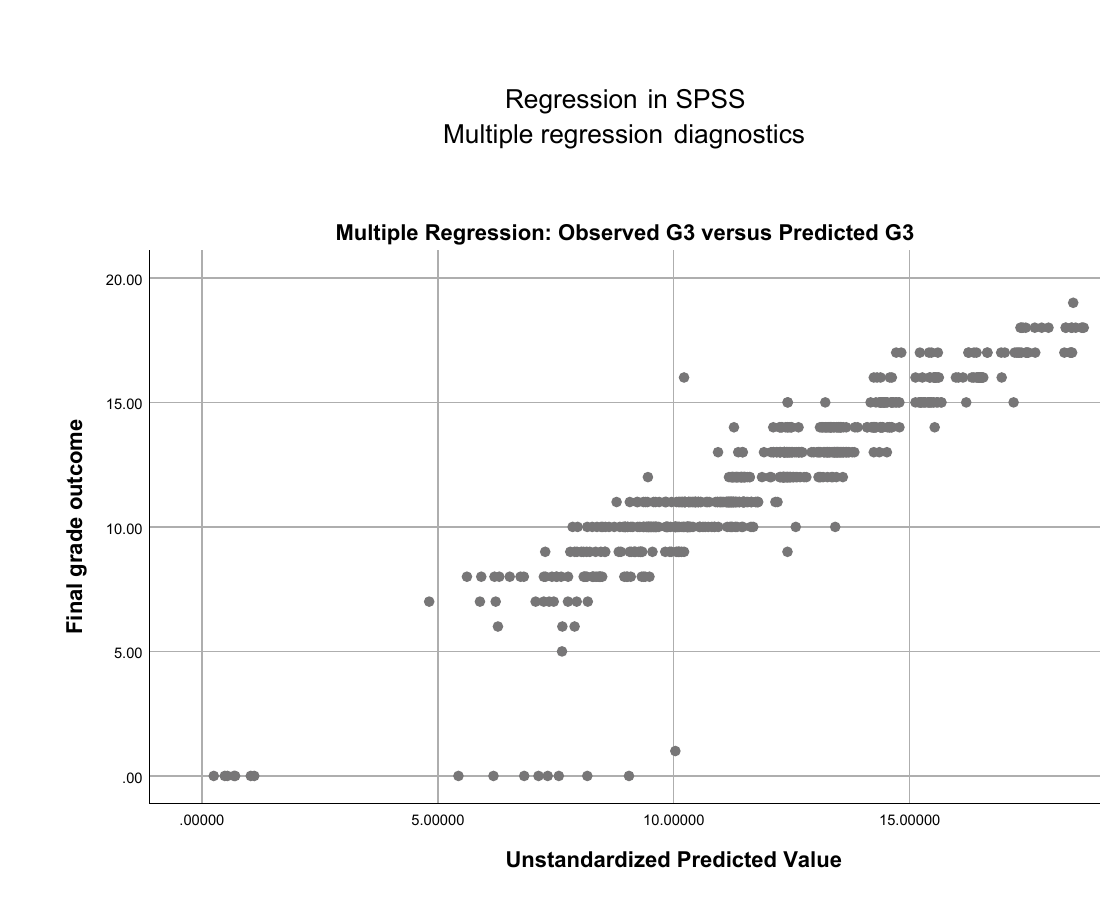
Most observations follow a strong increasing agreement pattern. The dense center is consistent with multiple R² = .851, but some cases remain far from the ideal observed-equals-predicted direction.
The Model Summary gives R = .922, R² = .851, adjusted R² = .849 and standard error = 1.25576 for 649 cases.
The chart describes fitted agreement in the analyzed cases. It does not show external prediction accuracy, and vertical error remains important for individual observations such as case 164.
Confirm that the chart pairs G3 with multi_pred, uses all 649 cases and follows the multiple ENTER procedure rather than the simple prediction variable.
SPSS Chart 2: Residuals Versus Predicted Values
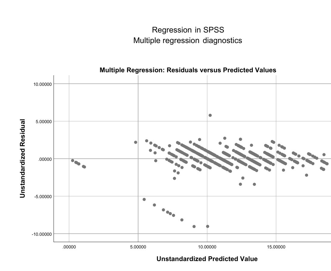
The zero-centered plot reveals the error structure across fitted values. Bands can arise because G3 is discrete, while changing spread, curvature and extreme negative errors require separate attention.
Raw residuals range from −9.05080 to 5.78244. The standard error of the estimate is 1.25576.
A centered cloud is desirable but does not by itself prove linearity, homoscedasticity, independence or normal residual tails.
Verify the command pairs multi_pred with multi_resid, inspect the most extreme points and join them to Cook’s distance and leverage.
SPSS Chart 3: Multiple-Model Residual Distribution
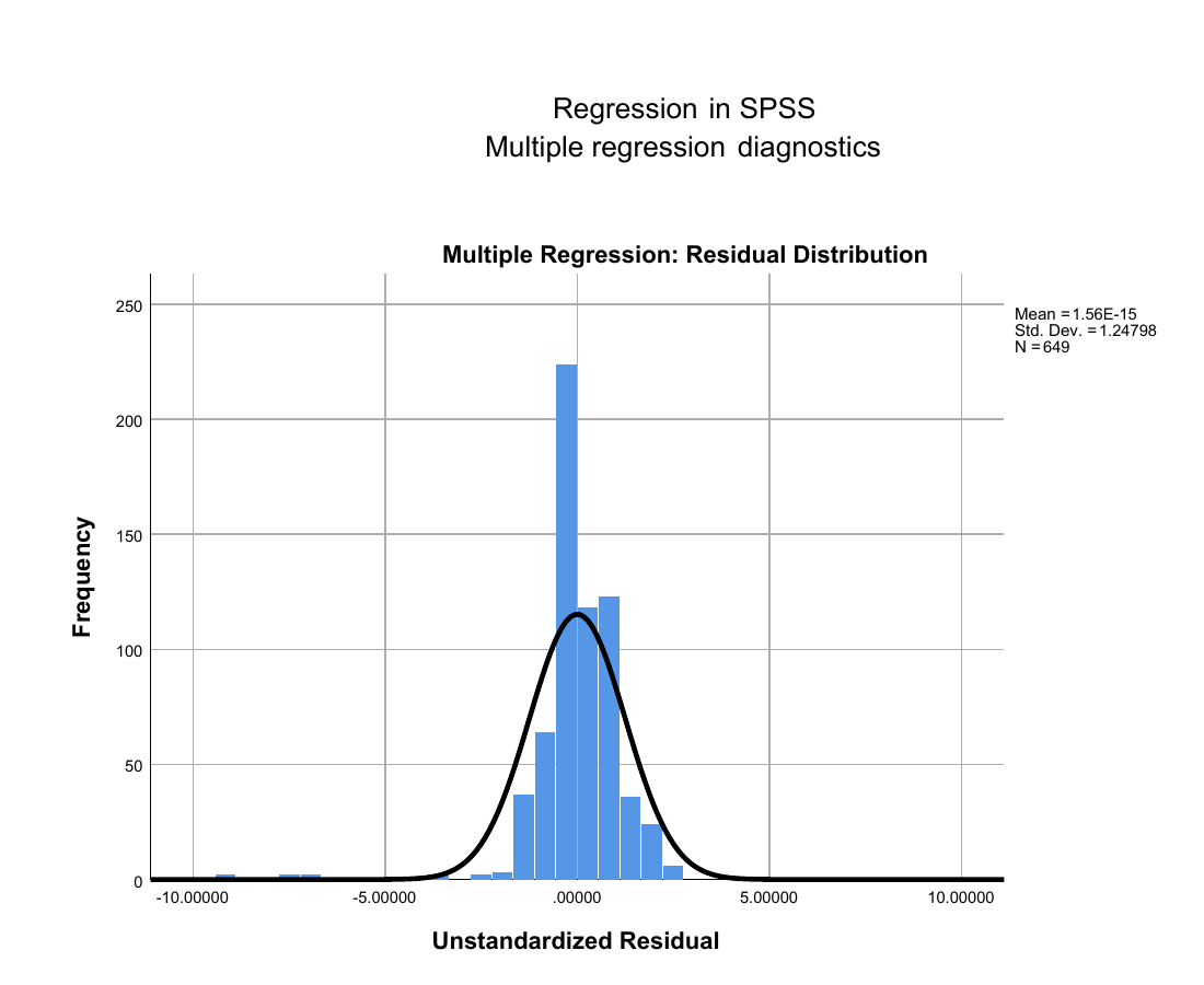
The main residual mass is concentrated near zero, but the negative tail is visibly extended by large underpredictions such as the −9.05080 residual.
The histogram should represent N = 649, with raw residual minimum −9.05080 and maximum 5.78244.
Residual shape affects classical reference inference and highlights observations requiring source and influence review. It does not mean that every coefficient estimate disappears.
Confirm the variable is multi_resid, inspect the normal probability plot and compare extreme residuals with studentized values, leverage and Cook’s distance.
Regression in SPSS Coefficient Interpretation
Regression in SPSS reports unstandardized B, standard error, standardized Beta, t, Sig., confidence intervals, zero-order correlation, partial correlation, part correlation, tolerance and VIF across the Coefficients table and its continuation.
Unstandardized B
B is used to reconstruct the fitted equation. Each multiple-model B is the expected G3 difference for a one-unit predictor contrast while all other listed predictors are fixed. B values cannot be ranked directly when predictors use different units.
Standardized Beta
Beta expresses the slope in standard-deviation units. G2 has Beta = .798 and G1 has Beta = .122, making G2 the dominant standardized predictor in the fitted model. Beta is sample dependent and is not a causal-importance score.
G2
G2 has B = .885, SE = .034, Beta = .798, t = 25.744 and a 95% interval from .817 to .952. Holding G1, studytime, failures, absences, age, Medu and Fedu constant, a one-point G2 difference is associated with an expected .885-point G3 difference.
G1
G1 has B = .143, Beta = .122 and an interval from .071 to .215. Its adjusted effect is smaller than its zero-order correlation with G3 because much of its grade information overlaps with G2.
Failures
Failures has B = −.235 and an interval from −.422 to −.048. At fixed values of the other predictors, one additional previous failure is associated with a lower expected G3. Its standardized magnitude is modest.
Absences
Absences has B = .023 and an interval from .001 to .044 even though its zero-order correlation with G3 is −.091. This sign change reflects conditioning and shared predictor structure. It is not evidence that absence improves achievement.
Uncertain Slopes
studytime, age, Medu and Fedu have displayed intervals containing zero. The overall model can be highly significant while several individual conditional slopes remain uncertain. The overall F test and individual t tests answer different questions.
Zero-Order, Partial and Part Correlations
The zero-order correlation describes the raw pair. The partial correlation removes the other predictors from both G3 and the focal predictor. The part correlation removes the other predictors only from the focal predictor and connects to the predictor’s unique increment in R² when squared under the corresponding model conditions.
Predictions, Effects and Model Meaning
Regression in SPSS saves fitted predictions directly into the active dataset. The multiple equation can therefore be audited row by row against multi_pred.
Reconstructing a Prediction
Use the unstandardized B values, not Beta. Small differences can occur when a prediction is recomputed from the three-decimal Viewer table because SPSS uses greater internal precision. The saved multi_pred value is the authoritative case-level result from the fitted procedure.
Residual Meaning
A negative residual means the observed G3 is below the predicted G3. Case 164 has observed 0, predicted 9.0508 and residual −9.05080. This is a large underprediction and should be investigated, but it does not automatically show a data error.
Prediction Versus Explanation
The equation describes fitted conditional association. It does not establish that intervening on G2, failures or absences would change G3 by the reported B. Experimental or causal interpretation requires design assumptions beyond the Linear Regression procedure.
Fitted Error Versus New-Case Accuracy
The standard error of the estimate and residual summaries describe the fitted cases. They are not holdout error. A prediction study requires a separate test sample or resampling process in which case selection and model fitting are repeated.
Feasible Outcome Range
Predicted values range from .2512 to 19.5507 in the saved output. These remain inside the observed grade scale for this sample, but an unconstrained linear equation can produce values outside a bounded outcome range for new predictor combinations. Review extrapolation before distributing a prediction tool.
Regression in SPSS Assumptions and Diagnostics
Regression in SPSS diagnostics should be read together. Model form, residual spread, residual distribution, dependence, collinearity, leverage and influence answer different questions.
Linearity
Review residuals versus predicted values for curvature and systematic structure. If a curve is visible, the additive linear equation may be incomplete. Candidate transformations or interactions should be justified by the research question and tested in a separate, clearly labeled procedure.
Homoscedasticity
Residual spread should remain reasonably stable over predicted values. A funnel or changing band width indicates unequal variance. The standard Linear Regression procedure does not automatically replace classical standard errors with a heteroscedasticity-robust covariance estimator.
Residual Distribution
The residual histogram and normal probability plot should be reviewed for symmetry and tail departures. The extreme negative residual range suggests that tail behavior is important. Residual non-normality does not erase the fitted B values, but it can weaken classical reference inference and highlight model or case problems.
Independence and Durbin-Watson
The multiple Durbin-Watson value is 1.862 and the simple value is 1.846. Values near two are often described as consistent with limited first-order autocorrelation, but the interpretation requires a meaningful case order. An arbitrary row order cannot establish independence.
VIF and Tolerance
G1 has tolerance .240 and VIF 4.165. G2 has tolerance .243 and VIF 4.121. These values show meaningful overlap, especially between prior-grade measures. They do not establish exact collinearity or require automatic deletion.
Condition Index
The maximum condition index is 56.814. A large index should be read with the variance proportions on the same dimension. In the verified output, the final dimension is dominated by the constant and age rather than showing several focal predictors with simultaneously large proportions. The maximum index alone is not a complete diagnosis.
Standardized and Studentized Residuals
Standardized residuals divide by a common estimate of residual spread. Studentized residuals account more directly for case leverage and are useful for unusual-case review. Keep the SPSS variable labels because the two quantities have different denominators.
Mahalanobis Distance
Mahalanobis distance identifies unusual combinations of predictor values. A high value means that a case lies far from the predictor center in multivariable space. It does not necessarily mean the observed outcome is poorly predicted.
Centered Leverage
The maximum centered leverage is .109. A screening threshold such as 2p/n depends on how p is defined and should be treated as contextual. Leverage identifies unusual predictor profiles; it does not measure outcome error directly.
Cook’s Distance
Cook’s distance combines residual discrepancy and leverage to estimate influence on the fitted equation. The maximum saved value is .147. Rules such as 4/n can identify many review candidates in a large sample and should not be converted into automatic deletion commands.
Casewise Diagnostics
The requested casewise table lists cases exceeding the standardized-residual threshold. Cases 62, 164 and 173 appear in the verified output. Review the original values, saved residuals, leverage and influence measures together, then refit sensitivity models if a valid observation appears materially influential.
Diagnostic Decision Table
| Output | Question | Appropriate action | Incorrect shortcut |
|---|---|---|---|
| Residual plot | Is the mean form or variance pattern incomplete? | Inspect structure, predictors and alternative specifications. | Declare assumptions satisfied because the mean residual is zero. |
| Histogram and P-P plot | Are residual shape and tails compatible with classical inference? | Review tails, cases and model form. | Delete cases until the graph looks normal. |
| VIF and tolerance | How much predictor information overlaps? | Discuss stability and substantive necessity. | Remove every predictor above one universal cutoff. |
| Condition index | Are several coefficients involved in near-dependence dimensions? | Read variance proportions on the same dimensions. | Use only the largest index. |
| Casewise diagnostics | Which cases have unusually large standardized residuals? | Trace source values and conduct sensitivity review. | Delete every listed case. |
| Cook and leverage | Which cases may affect the equation? | Inspect jointly with residuals and data validity. | Interpret influence as proof of error. |
| Durbin-Watson | Is first-order residual ordering relevant? | Interpret only with meaningful order and design context. | Use the number to prove general independence. |
SPSS Workflow and Reproducibility
Regression in SPSS is reproducible when the dataset state, syntax, output and saved diagnostic variables are controlled as one package.
Data Editor
- Verify variable names and types.
- Review labels and user-missing values.
- Confirm filter, weighting and Split File are off.
- Preserve a source dataset without generated diagnostics.
Syntax Editor
- Records the exact dependent variable.
- Records METHOD=ENTER and predictor order.
- Records statistics, casewise and save options.
- Supports a clean top-to-bottom rerun.
Output Viewer
- Preserves Notes, tables and chart objects.
- Shows table continuations and footnotes.
- Supports native SPV review.
- Requires provenance checks when old output remains.
Exported PDF
- Provides a stable reading copy.
- Can split wide tables across pages.
- Can retain stale pages if the Viewer was not cleaned.
- Should be inspected after export.
Recommended Clean Rerun
- Start a new SPSS session.
- Close all datasets and Viewer output.
- Import the correct dataset.csv from the regression folder.
- Name the active dataset clearly.
- Verify 649 cases and the nine analysis variables.
- Run descriptives and correlations.
- Run the simple ENTER procedure and save simple diagnostics.
- Run the multiple ENTER procedure and save eight diagnostics.
- Create charts from the named saved variables.
- Save the augmented SAV separately.
- Save the SPV.
- Export the complete output to PDF with compatibility-safe syntax.
- Inspect the first pages, table continuations, chart titles and final page.
Output Reconciliation Checks
- Both Model Summary tables should report 649 valid cases through their Notes and df.
- The multiple procedure must list eight entered predictors.
- Total df must equal 648 and residual df must equal 640.
- Regression SS 5754.033 plus residual SS 1009.234 must equal total SS 6763.267 within rounding.
- The Coefficients table must contain the constant and eight predictor rows.
- G1 and G2 tolerance and VIF must be read from the matching multiple coefficient table.
multi_residmust equal observed G3 minusmulti_pred.- The page 81 chart must use G3 and
multi_pred. - The page 83 chart must use
multi_predandmulti_resid. - The page 87 histogram must use
multi_resid. - Casewise entries must trace to the active dataset without a filter or Split File.
Corrected SPSS Syntax
Regression in SPSS syntax below removes the stale placeholder paths visible in the old setup record, uses the correct regression folder consistently, closes prior datasets and output, runs both models and applies compatibility-safe SAV, SPV and PDF exports.
Complete SPSS regression syntax
* Regression in SPSS - corrected reproducible syntax.
* Target folder:
* D:\DATA ANALYSIS\H Regression Tests and Models\Regression in SPSS.

DATASET CLOSE ALL.
OUTPUT CLOSE ALL.
SET UNICODE=ON.
SET DECIMAL=DOT.
SET OLANG=ENGLISH.
SET MPRINT=ON.
SET PRINTBACK=ON.
OMSEND.

* Create output folders when needed.
HOST COMMAND=[
'if not exist "D:\DATA ANALYSIS\H Regression Tests and Models\Regression in SPSS\SPSS_Output\sav" mkdir "D:\DATA ANALYSIS\H Regression Tests and Models\Regression in SPSS\SPSS_Output\sav"'
].
HOST COMMAND=[
'if not exist "D:\DATA ANALYSIS\H Regression Tests and Models\Regression in SPSS\SPSS_Output\spv" mkdir "D:\DATA ANALYSIS\H Regression Tests and Models\Regression in SPSS\SPSS_Output\spv"'
].
HOST COMMAND=[
'if not exist "D:\DATA ANALYSIS\H Regression Tests and Models\Regression in SPSS\SPSS_Output\pdf" mkdir "D:\DATA ANALYSIS\H Regression Tests and Models\Regression in SPSS\SPSS_Output\pdf"'
].

* Remove prior generated outputs.
HOST COMMAND=[
'del /Q "D:\DATA ANALYSIS\H Regression Tests and Models\Regression in SPSS\SPSS_Output\sav\*.sav" 2>nul'
].
HOST COMMAND=[
'del /Q "D:\DATA ANALYSIS\H Regression Tests and Models\Regression in SPSS\SPSS_Output\spv\*.spv" 2>nul'
].
HOST COMMAND=[
'del /Q "D:\DATA ANALYSIS\H Regression Tests and Models\Regression in SPSS\SPSS_Output\pdf\*.pdf" 2>nul'
].

* Import dataset.csv.
GET DATA
 /TYPE=TXT
 /FILE='D:\DATA ANALYSIS\H Regression Tests and Models\Regression in SPSS\dataset.csv'
 /ENCODING='UTF8'
 /DELCASE=LINE
 /DELIMITERS=","
 /QUALIFIER='"'
 /ARRANGEMENT=DELIMITED
 /FIRSTCASE=2
 /IMPORTCASE=ALL
 /VARIABLES=
  school A8
  sex A8
  age F8.0
  address A8
  famsize A8
  Pstatus A8
  Medu F8.0
  Fedu F8.0
  Mjob A16
  Fjob A16
  reason A16
  guardian A16
  traveltime F8.0
  studytime F8.0
  failures F8.0
  schoolsup A8
  famsup A8
  paid A8
  activities A8
  nursery A8
  higher A8
  internet A8
  romantic A8
  famrel F8.0
  freetime F8.0
  goout F8.0
  Dalc F8.0
  Walc F8.0
  health F8.0
  absences F8.0
  G1 F8.2
  G2 F8.2
  G3 F8.2.
CACHE.
EXECUTE.

DATASET NAME RegressionInSPSSData WINDOW=FRONT.

VARIABLE LABELS
 G3 'Final grade outcome'
 G1 'First-period grade predictor'
 G2 'Second-period grade predictor'
 studytime 'Weekly study-time predictor'
 failures 'Past class failures predictor'
 absences 'School absences predictor'
 age 'Student age predictor'
 Medu 'Mother education predictor'
 Fedu 'Father education predictor'.

VARIABLE LEVEL
 G3 G1 G2 studytime failures absences age Medu Fedu (SCALE).

FORMATS
 G3 G1 G2 studytime failures absences age Medu Fedu (F8.2).

EXECUTE.

TITLE 'Regression in SPSS'.
SUBTITLE 'Descriptive statistics and correlations'.

FREQUENCIES VARIABLES=
 G3 G1 G2 studytime failures absences age Medu Fedu
 /FORMAT=NOTABLE
 /STATISTICS=MINIMUM MAXIMUM MEAN STDDEV SKEWNESS KURTOSIS
 /ORDER=ANALYSIS.

DESCRIPTIVES VARIABLES=
 G3 G1 G2 studytime failures absences age Medu Fedu
 /STATISTICS=MEAN STDDEV MIN MAX SKEWNESS KURTOSIS.

CORRELATIONS
 /VARIABLES=G3 G1 G2 studytime failures absences age Medu Fedu
 /PRINT=TWOTAIL SIG
 /MISSING=PAIRWISE.

* Simple linear regression.
TITLE 'Regression in SPSS'.
SUBTITLE 'Simple model: G3 predicted by G2'.

REGRESSION
 /MISSING LISTWISE
 /STATISTICS COEFF OUTS R ANOVA CHANGE CI(95) ZPP
 /CRITERIA=PIN(.05) POUT(.10) TOLERANCE(.0001)
 /NOORIGIN
 /DEPENDENT G3
 /METHOD=ENTER G2
 /RESIDUALS DURBIN
 /CASEWISE PLOT(ZRESID) OUTLIERS(3)
 /SAVE
  PRED(simple_pred)
  RESID(simple_resid)
  ZPRED(simple_zpred)
  ZRESID(simple_zresid).

TITLE 'Regression in SPSS'.
SUBTITLE 'Simple model diagnostics'.

DESCRIPTIVES VARIABLES=
 simple_pred simple_resid simple_zpred simple_zresid
 /STATISTICS=MEAN STDDEV MIN MAX.

EXAMINE VARIABLES=simple_resid simple_zresid
 /PLOT BOXPLOT HISTOGRAM NPPLOT
 /STATISTICS DESCRIPTIVES EXTREME
 /CINTERVAL 95
 /MISSING LISTWISE
 /NOTOTAL.

GRAPH
 /SCATTERPLOT(BIVAR)=G2 WITH G3
 /TITLE='Simple Regression: G3 by G2'.

GRAPH
 /SCATTERPLOT(BIVAR)=simple_pred WITH G3
 /TITLE='Simple Regression: Observed and Predicted G3'.

GRAPH
 /SCATTERPLOT(BIVAR)=simple_pred WITH simple_resid
 /TITLE='Simple Regression: Residuals and Predictions'.

GRAPH
 /HISTOGRAM(NORMAL)=simple_resid
 /TITLE='Simple Regression: Residual Distribution'.

* Multiple linear regression.
TITLE 'Regression in SPSS'.
SUBTITLE 'Multiple ENTER model predicting G3'.

REGRESSION
 /MISSING LISTWISE
 /STATISTICS COEFF OUTS R ANOVA CHANGE CI(95) COLLIN TOL ZPP
 /CRITERIA=PIN(.05) POUT(.10) TOLERANCE(.0001)
 /NOORIGIN
 /DEPENDENT G3
 /METHOD=ENTER G1 G2 studytime failures absences age Medu Fedu
 /RESIDUALS DURBIN
 /CASEWISE PLOT(ZRESID) OUTLIERS(3)
 /SAVE
  PRED(multi_pred)
  RESID(multi_resid)
  ZPRED(multi_zpred)
  ZRESID(multi_zresid)
  SRESID(multi_sresid)
  MAHAL(multi_mahal)
  COOK(multi_cook)
  LEVER(multi_lev).

TITLE 'Regression in SPSS'.
SUBTITLE 'Multiple model residual and influence diagnostics'.

DESCRIPTIVES VARIABLES=
 multi_pred multi_resid multi_zpred multi_zresid multi_sresid
 multi_mahal multi_cook multi_lev
 /STATISTICS=MEAN STDDEV MIN MAX.

EXAMINE VARIABLES=
 multi_resid multi_zresid multi_sresid multi_mahal multi_cook multi_lev
 /PLOT BOXPLOT HISTOGRAM NPPLOT
 /STATISTICS DESCRIPTIVES EXTREME
 /CINTERVAL 95
 /MISSING LISTWISE
 /NOTOTAL.

* Add contextual screening indicators.
AGGREGATE
 /OUTFILE=* MODE=ADDVARIABLES
 /BREAK=
 /regression_n=N.

COMPUTE leverage_threshold = 2 * (8 + 1) / regression_n.
COMPUTE cooks_threshold = 4 / regression_n.
COMPUTE high_leverage = (multi_lev > leverage_threshold).
COMPUTE high_cooks = (multi_cook > cooks_threshold).
COMPUTE large_std_residual_2 = (ABS(multi_zresid) > 2).
COMPUTE large_std_residual_3 = (ABS(multi_zresid) > 3).

VARIABLE LABELS
 regression_n 'Number of complete regression cases'
 leverage_threshold 'Context threshold: 2p divided by n'
 cooks_threshold 'Context threshold: 4 divided by n'
 high_leverage '1 = leverage exceeds context threshold'
 high_cooks '1 = Cook distance exceeds context threshold'
 large_std_residual_2 '1 = absolute standardized residual exceeds 2'
 large_std_residual_3 '1 = absolute standardized residual exceeds 3'.

VALUE LABELS
 high_leverage high_cooks large_std_residual_2 large_std_residual_3
 0 'No'
 1 'Yes'.

EXECUTE.

FREQUENCIES VARIABLES=
 high_leverage high_cooks large_std_residual_2 large_std_residual_3
 /ORDER=ANALYSIS.

GRAPH
 /SCATTERPLOT(BIVAR)=multi_pred WITH G3
 /TITLE='Multiple Regression: Observed and Predicted G3'.

GRAPH
 /SCATTERPLOT(BIVAR)=multi_pred WITH multi_resid
 /TITLE='Multiple Regression: Residuals and Predictions'.

GRAPH
 /HISTOGRAM(NORMAL)=multi_resid
 /TITLE='Multiple Regression: Residual Distribution'.

* Save augmented data.
SAVE OUTFILE=
 'D:\DATA ANALYSIS\H Regression Tests and Models\Regression in SPSS\SPSS_Output\sav\regression_in_spss_analysis_data.sav'
 /COMPRESSED.

* Save native Viewer and export compatibility-safe PDF.
OUTPUT SAVE OUTFILE=
 'D:\DATA ANALYSIS\H Regression Tests and Models\Regression in SPSS\SPSS_Output\spv\regression_in_spss_output.spv'.

OUTPUT EXPORT
 /CONTENTS EXPORT=ALL LAYERS=PRINTSETTING MODELVIEWS=PRINTSETTING
 /PDF DOCUMENTFILE=
 'D:\DATA ANALYSIS\H Regression Tests and Models\Regression in SPSS\SPSS_Output\pdf\regression_in_spss_output.pdf'.
The threshold indicators are screening aids. They do not authorize automatic case removal. Review data validity, substantive relevance and sensitivity results.
Minimal simple regression command
REGRESSION
 /MISSING LISTWISE
 /STATISTICS COEFF OUTS R ANOVA CHANGE CI(95) ZPP
 /NOORIGIN
 /DEPENDENT G3
 /METHOD=ENTER G2
 /RESIDUALS DURBIN
 /CASEWISE PLOT(ZRESID) OUTLIERS(3)
 /SAVE PRED(simple_pred) RESID(simple_resid)
       ZPRED(simple_zpred) ZRESID(simple_zresid).
The simple procedure establishes the G2-only benchmark and saves the variables required for a case-level audit.
Minimal multiple regression command
REGRESSION
 /MISSING LISTWISE
 /STATISTICS COEFF OUTS R ANOVA CHANGE CI(95) COLLIN TOL ZPP
 /NOORIGIN
 /DEPENDENT G3
 /METHOD=ENTER G1 G2 studytime failures absences age Medu Fedu
 /RESIDUALS DURBIN
 /CASEWISE PLOT(ZRESID) OUTLIERS(3)
 /SAVE PRED(multi_pred) RESID(multi_resid)
       ZPRED(multi_zpred) ZRESID(multi_zresid)
       SRESID(multi_sresid) MAHAL(multi_mahal)
       COOK(multi_cook) LEVER(multi_lev).
This command requests the verified ENTER model, confidence intervals, collinearity statistics, correlations, Durbin-Watson and saved diagnostics.
Case-level equation audit
COMPUTE equation_pred =
 -.501155
 + .143397 * G1
 + .884807 * G2
 + .096632 * studytime
 - .235361 * failures
 + .022762 * absences
 + .022685 * age
 - .044951 * Medu
 + .022025 * Fedu.

COMPUTE equation_difference = multi_pred - equation_pred.
DESCRIPTIVES VARIABLES=equation_difference
 /STATISTICS=MEAN STDDEV MIN MAX.
The displayed coefficients are rounded in the article. For an exact zero difference, use full-precision B values from a machine-readable coefficient export or SPSS transformation output.
Compatibility-safe SPSS output export
OUTPUT SAVE OUTFILE=
 'D:\DATA ANALYSIS\H Regression Tests and Models\Regression in SPSS\SPSS_Output\spv\regression_in_spss_output.spv'.

OUTPUT EXPORT
 /CONTENTS EXPORT=ALL LAYERS=PRINTSETTING MODELVIEWS=PRINTSETTING
 /PDF DOCUMENTFILE=
 'D:\DATA ANALYSIS\H Regression Tests and Models\Regression in SPSS\SPSS_Output\pdf\regression_in_spss_output.pdf'.
This block avoids unsupported standalone bookmark or font subcommands and preserves the native SPV before PDF export.
Advanced Regression in SPSS Topics
Regression in SPSS requires additional care when wide Viewer tables, ordered codes, collinearity dimensions, influence thresholds and validation claims are involved.
Sig. .000 Is Not Zero
SPSS displays very small probabilities as .000 at the default precision. Report p < .001. Writing p = 0 is mathematically incorrect and overstates what the Viewer displays.
B Versus Beta
B retains original units and belongs in the prediction equation. Beta is standardized and supports relative scale comparison inside the fitted sample. A Beta of .798 for G2 does not mean that G2 causes 79.8% of G3.
R² Versus Percentage of Correct Predictions
R² = .851 means that approximately 85.1% of corrected sample variation in G3 is represented by the fitted equation. It does not mean that 85.1% of individual grades are predicted correctly.
Standard Error of the Estimate
The multiple standard error of 1.25576 is derived using residual degrees of freedom. It describes fitted residual scale under the procedure. It is not identical to a mean-squared-error calculation using n and is not an external test error.
ENTER Versus Stepwise Selection
METHOD=ENTER retains the prespecified predictor block. Stepwise methods use sample criteria to add or remove terms and would produce a different inferential process. Do not call the verified result stepwise.
Ordered Codes Entered as Scale Terms
studytime, Medu and Fedu are entered as numeric linear terms. This assumes that a one-code increase has a constant slope. Treating them as categorical predictors would require dummy variables and a different interpretation.
Pairwise Correlations Versus Listwise Regression
The correlation command requests pairwise deletion while REGRESSION uses listwise deletion. All nine columns are complete in this output, so N remains 649. In another dataset, the correlation and regression tables could describe different cases.
Condition Index and Variance Proportions
A large condition index is concerning only in context. Review which coefficient variance proportions concentrate on the same high-index dimension. The maximum 56.814 should not be reported as a stand-alone declaration of fatal collinearity.
Leverage Threshold Definitions
Rules using 2p/n or 3p/n vary in whether p includes the intercept. State the chosen definition. In the corrected syntax, p is treated as eight predictors plus the intercept for the displayed context threshold.
Cook’s Distance Thresholds
The rule 4/n is a sensitive screening convention, not a universal deletion threshold. In a sample of 649 it can flag cases whose influence remains modest. Compare the maximum .147 with coefficient sensitivity and source validity.
Casewise Output and Source Rows
SPSS case numbers can change when sorting, filtering or selecting cases. Preserve a stable source identifier. Do not assume that case number 164 will remain the same after rearranging the dataset.
Chart Axis Pairing
The GRAPH command places the first named variable on one axis and the second on the other according to command conventions and chart output. Confirm the displayed labels instead of inferring orientation from the syntax line alone.
Viewer Table Continuations
Wide coefficient and collinearity tables can continue across pages. Record coefficient rows, intervals, correlations, tolerance and VIF only after confirming that continuation pages refer to the same model.
Stale Output Pages
Closing old Viewer output before rerunning prevents unrelated Notes and HOST records from entering the PDF. The existing 95-page file discloses its stale first pages; a corrected rerun should create a clean output from the start.
Source and Augmented SAV Files
The source SAV or imported dataset should remain unchanged. Save predicted and diagnostic variables to a separate augmented SAV. This prevents generated variables from being mistaken for original observations during a later analysis.
Validation
The Viewer reports fitted performance. A validation study requires cases not used to estimate the equation or a resampling design. Predictor selection, transformations and data preparation must be repeated inside the validation process.
Common Regression in SPSS Mistakes
Procedure and output mistakes
- Leaving an old filter, weight or Split File active.
- Using the wrong active dataset.
- Running the dialog without saving syntax.
- Reading only the first page of a continued table.
- Mixing simple and multiple saved residual variables.
- Exporting a Viewer containing unrelated earlier output.
Interpretation mistakes
- Reporting Sig. .000 as p = 0.
- Using Beta in the prediction equation.
- Calling R² a percentage of correct predictions.
- Calling adjusted association causal.
- Deleting every high-VIF predictor automatically.
- Deleting every case above a residual or Cook threshold.
Regression in SPSS Decision Rules
- Verify the active dataset and Notes before reading any table.
- Report METHOD=ENTER and the complete predictor list.
- Read Model Summary, ANOVA and Coefficients as different evidence.
- Use B for the fitted equation and Beta for supplementary comparison.
- Report p < .001 when SPSS displays .000.
- Read VIF with tolerance and condition diagnostics.
- Read residual size with leverage and Cook’s distance.
- Trace case numbers to stable source identifiers.
- Keep fitted error separate from validation error.
- Archive syntax, source data, augmented SAV, SPV and PDF.
- Regression in SPSS should start with DATASET CLOSE ALL and OUTPUT CLOSE ALL in a clean rerun.
- Regression in SPSS should record the active dataset and valid case count.
- Regression in SPSS should preserve METHOD=ENTER in both syntax and reporting.
- Regression in SPSS should reconcile ANOVA sums of squares and degrees of freedom.
- Regression in SPSS should use B, not Beta, for predictions.
- Regression in SPSS should save residual and influence variables with clear prefixes.
- Regression in SPSS should interpret VIF and condition indices together.
- Regression in SPSS should treat case thresholds as screening rules.
- Regression in SPSS should exclude stale Viewer pages from substantive evidence.
- Regression in SPSS should label fitted accuracy as in-sample.
- Regression in SPSS should identify the active dataset before every procedure.
- Regression in SPSS should preserve METHOD=ENTER in syntax and reporting.
- Regression in SPSS should reconcile Model Summary, ANOVA and Coefficients tables.
- Regression in SPSS should use B for predictions and Beta for standardized comparison.
- Regression in SPSS should save predictions, residuals, leverage and influence variables.
- Regression in SPSS should interpret diagnostic thresholds as review rules.
- Regression in SPSS should exclude stale Viewer pages from substantive evidence.
- Regression in SPSS should label the reported error as fitted-sample evidence.
APA-Style Reporting
Regression in SPSS reporting should identify the dependent variable, entry method, predictor block, sample, fit, coefficient evidence and diagnostic limitations.
Diagnostic Reporting Example
Collinearity review indicated substantial overlap between G1 and G2, with VIF values of 4.165 and 4.121, respectively. The maximum condition index was 56.814 and was interpreted with the associated variance proportions rather than as a stand-alone decision. Multiple-model residuals ranged from −9.05080 to 5.78244, the maximum Cook’s distance was .147 and maximum centered leverage was .109. Case 164 had observed G3 = 0 and predicted G3 = 9.0508 and was retained for source and sensitivity review rather than automatically excluded.
Viewer Provenance Statement
The exported Viewer PDF contained stale setup notes on its opening pages. Those pages were excluded from statistical evidence. The reported results were taken from the applicable record beginning with the correct regression import and the Notes, syntax and tables identifying the 649-case Regression in SPSS analysis.
Publication Checklist
Regression in SPSS should pass the following checks before publication.
- State G3 as the dependent variable.
- List G1, G2, studytime, failures, absences, age, Medu and Fedu.
- State that METHOD=ENTER was used.
- Report 649 valid cases.
- Report simple and multiple Model Summary values accurately.
- Report F with correct degrees of freedom.
- Write p < .001 rather than p = 0 for Sig. .000.
- Report B, Beta, confidence intervals and units correctly.
- Explain the conditional positive absences coefficient cautiously.
- Report G1 and G2 tolerance and VIF values.
- Explain the condition-index limitation.
- Report residual, Cook and leverage extremes.
- Discuss case 164 without automatic deletion.
- Verify all three SPSS chart URLs and page references.
- Disclose the stale opening PDF pages.
- Verify the output PDF download.
- Retain all advertisement placements and the back-to-top control.
Downloads and SPSS Chart Resources
Regression in SPSS downloads are restricted to the verified SPSS Viewer PDF and the three extracted same-run chart pages.
Observed versus predicted chartViewer page 81 multiple-model comparison
Residuals versus predicted chartViewer page 83 residual-pattern diagnostic
Residual distribution chartViewer page 87 multiple-model histogram
Frequently Asked Questions
Regression in SPSS questions below address the settings and interpretations most likely to change the reported result.
Why does the SPSS PDF begin with another folder path?
The opening HOST notes came from an earlier output state. They are disclosed and excluded. The applicable analysis begins with the correct regression import and later Notes tables showing the correct dataset and 649 cases.
What does Sig. .000 mean?
It means the probability is smaller than SPSS displays at the chosen precision. Report p < .001, not p = 0.
Did SPSS use stepwise selection?
No. Both procedures use METHOD=ENTER. The multiple procedure enters all eight specified predictors simultaneously.
What is the difference between B and Beta?
B is the original-unit coefficient used in the fitted equation. Beta is standardized and supports relative magnitude comparison inside the fitted model.
Why is R² .851 not 85.1% correct predictions?
R² describes the proportion of corrected sample variation represented by the model. It is not a classification accuracy measure or a count of exactly predicted grades.
Why are several residual variables saved?
Raw, standardized and studentized residuals use different scales. Predicted values, Mahalanobis distance, Cook’s distance and leverage answer complementary diagnostic questions.
Is VIF 4.165 acceptable?
It indicates substantial overlap and should be discussed. It does not by itself require deleting G1 or G2. Predictor stability and the research question matter.
Does condition index 56.814 prove fatal collinearity?
No. Condition indices must be read with coefficient variance proportions on the same dimensions. The maximum value alone is incomplete evidence.
Should case 164 be deleted?
No automatic deletion is justified. Check the source record, determine whether it is valid, examine leverage and Cook’s distance, and report sensitivity results.
What is the difference between residual and studentized residual?
The raw residual is observed minus predicted on the G3 scale. A studentized residual divides the error by a case-specific estimated standard error that accounts for leverage.
Does Durbin-Watson 1.862 prove independence?
No. It is near two, but its substantive interpretation requires a meaningful observation order. Independence also depends on sampling and clustering.
Can the standard error 1.25576 be reported as future prediction error?
No. It describes fitted residual scale. Future performance requires a validation sample or a correctly designed resampling analysis.
Which files preserve the complete SPSS analysis?
The syntax preserves the commands, the source data preserve the original measurements, the augmented SAV preserves saved diagnostics, the SPV preserves native output and the PDF provides a stable review copy.
Why should output be closed before a rerun?
Closing old output prevents stale tables and HOST notes from being mixed into the new Viewer and exported PDF.
Regression in SPSS Conclusion
Regression in SPSS verifies a strong fitted grade model. The simple G2 procedure reports R² = .844, and the multiple eight-predictor ENTER procedure reports R² = .851, adjusted R² = .849, standard error = 1.25576 and F(8, 640) = 456.111, p < .001.
G2 is the dominant standardized predictor with Beta = .798. G1 contributes a smaller positive conditional coefficient, failures has a negative coefficient and absences has a small positive adjusted coefficient that must not be interpreted causally. G1 and G2 VIF values near four show substantial shared information.
The Viewer also preserves important limitations. Residuals range from −9.05080 to 5.78244, Cook’s distance reaches .147, centered leverage reaches .109 and case 164 is underpredicted by more than nine grade points. These values support case and sensitivity review even though overall fitted strength is high.
The main practical strength of Regression in SPSS is its connected audit trail: the syntax declares the procedure, the Notes tables identify the data state, the Model Summary and ANOVA establish fit, the Coefficients table reports conditional slopes, saved variables support case diagnostics and the SPV preserves the native record.

