
Regression in R: lm Formula, Diagnostics, Interpretation, Code and Reproducible Results
Regression in R is presented here as a complete, R-only workflow. The guide follows the verified 649-row analysis from data classes and complete-case construction through simple and multiple lm objects, coefficient interpretation, ANOVA, residual diagnostics, VIF, influence checks, reproducible tables, ten R charts and the saved report.
Simple and multiple lm fits
10 verified R charts
Exact R output anchors
Regression in R Model Overview
Regression in R connects the research formula with the exact model frame and design matrix used for estimation.
Regression in R estimates a continuous conditional mean through an explicit formula and a model frame that records the response, predictors and observations actually used. The verified simple object fits G3 ~ G2. The verified multiple object fits G3 ~ G1 + G2 + studytime + failures + absences + age + Medu + Fedu.
Both objects use the same 649 complete observations. That fixed analysis frame is essential: a comparison of R-squared, RMSE or residual behavior is meaningful only when the response rows are identical. The richer formula raises fitted R-squared from 0.843730 to 0.850777 and reduces fitted RMSE from 1.276125 to 1.247020, but the improvement remains an in-sample comparison rather than a future-cohort validation result.
What Is Regression in R?
Regression in R normally uses lm() for ordinary least squares. The function converts the formula and data into a design matrix, estimates coefficients through stable numerical routines, stores fitted values and residuals, and provides methods for summaries, intervals, predictions and diagnostic quantities.
When Should Regression in R Be Used?
Good uses
- Fitting transparent simple and multiple linear models.
- Controlling formula terms, factors, interactions and transformations.
- Extracting exact tables rather than relying on screenshots.
- Creating reproducible predictions, residuals and influence audits.
- Extending the baseline with robust uncertainty or validation procedures.
Weak uses
- Applying
lmto an outcome requiring a different model family. - Comparing candidate models fitted on different observations.
- Interpreting a conditional slope as a causal effect without design support.
- Calling fitted RMSE expected error for unseen data.
- Running code without checking imported classes, contrasts or missing values.
Core Assumptions and Requirements
1. Correct continuous-outcome model
G3 is treated as a continuous outcome. A binary, count, ordinal, censored or survival outcome requires a model whose scale and likelihood match that structure.
2. One controlled model frame
Every compared fit should use the same eligible rows. model.frame(), nobs() and the exported case-level table should all report 649 observations.
3. Linear conditional mean
The mean of G3 should be adequately represented by the declared additive linear formula. Residual-versus-fitted evidence is used to review curvature and systematic structure.
4. Independent observations
The design should support independence. Row order and clustering cannot be repaired by a syntactically correct formula.
5. Appropriate residual variance
Classical standard errors assume a variance structure compatible with ordinary least squares. The saved Breusch-Pagan result warns that constant variance is doubtful.
6. No exact linear dependence
The design matrix must have full estimable rank. G1 and G2 overlap strongly, but their VIF values near four do not indicate exact duplication.
7. Reproducible object and environment
The formula, data preparation, package versions, diagnostic definitions and exported values should be regenerated from a clean session.
Quick Answer
Regression in R should be interpreted from fit, coefficients and diagnostics together rather than from one headline statistic.
Regression in R gives a strong fitted relationship for the saved 649-row model frame, with G2 providing most of the standardized predictive signal. The residual evidence, however, warns against reporting the classical model as assumption-free or externally validated.
What the verified R output supports
- Both fitted objects use 649 complete rows.
- The eight-predictor formula explains 85.08% of fitted G3 variation.
- The complete slope block is statistically significant.
- G2 has the largest standardized coefficient.
- G1, G2, failures and absences have saved 95% intervals excluding zero.
- The exact object outputs can be regenerated and exported.
What the verified R output does not prove
- It does not establish causality.
- It does not prove that every included predictor is important.
- It does not guarantee RMSE = 1.247020 in an unseen cohort.
- It does not remove the heteroscedasticity and tail warnings.
- It does not make arbitrary row order meaningful for serial-correlation interpretation.
- It does not justify automatic deletion of influential observations.
Table of Contents
Regression in R is organized below from data preparation through reproducible reporting.
- Why this analysis needs Regression in R
- How Regression in R works
- R object structure and audit trail
- Variables, classes and complete cases
- Regression in R results
- Ten R charts and explanations
- Coefficient interpretation
- Predictions and effects
- Assumptions and diagnostics
- R procedures and reproducibility
- R code panels
- Advanced Regression in R topics
- APA-style reporting
- Publication checklist
- Downloads and chart resources
- Related Salar Cafe guides
- Frequently asked questions
- Regression in R conclusion
Why This Analysis Needs Regression in R
Regression in R keeps the simple baseline and conditional multiple model in one auditable environment.
Regression in R is useful here because the research question requires both a readable model formula and an auditable object containing the exact model frame. The simple formula estimates the G2-only association. The multiple formula estimates eight slopes simultaneously and therefore changes each coefficient into a conditional contrast.
The substantive question is not merely whether G2 correlates with G3. The multiple object asks how expected G3 differs with G2 among records with the same G1, studytime, failures, absences, age, Medu and Fedu. That conditional estimand is the reason the formula, coding and predictor overlap must be reported.
Regression in R also makes a strong baseline easy to preserve. A later robust covariance estimate, transformed equation or validation analysis can be compared with the same verified lm object rather than replacing the original result without an audit trail.
How Regression in R Works
Regression in R remains reproducible when all tables and charts are generated from named fitted objects.
Regression in R moves through three connected stages: prepare the analysis frame, estimate the declared formula, and obtain all interpretation and diagnostics from the resulting object.
Set classes, select nine variables and apply one complete-case rule.
Estimate simple and multiple formulas on the same 649 observations.
Export coefficients, ANOVA, predictions, diagnostics and charts from those fits.
Formula Interface
The formula G3 ~ G1 + G2 + studytime + failures + absences + age + Medu + Fedu requests an intercept and eight additive slopes. The tilde separates the response from the right-hand-side terms. The plus signs add columns to the design matrix; they do not fit eight independent bivariate regressions.
Formula operators can change the model materially. G1 * G2 expands to G1, G2 and their interaction. I(G2^2) adds a squared numeric term. A factor generates indicator columns according to its contrasts. These changes must be intentional and visible in the reported equation.
Model Frame and Design Matrix
model.frame(fit) shows the variables and observations used after formula evaluation and missing-data handling. model.matrix(fit) shows the actual columns estimated, including the intercept, factor indicators, transformations and interactions. These functions are more reliable than assuming that imported column names equal the fitted design.
Because both verified models use the same rows, the difference in fitted statistics reflects the formula rather than a changing sample. This same-frame requirement is especially important when candidate predictors contain different missing-value patterns.
Ordinary Least Squares Estimator
lm() estimates the coefficients that minimize the residual sum of squares. The familiar expression \(\hat{\beta}=(X’X)^{-1}X’y\) describes the solution when the matrix is invertible, but R uses stable matrix decomposition rather than requiring a manual inverse.
Simple and Multiple Objects
The simple object has one slope and 647 residual degrees of freedom. The multiple object has eight slopes, an intercept and 640 residual degrees of freedom. The multiple R-squared is larger by about 0.007047 and its fitted RMSE is lower by about 0.029104. This improvement is modest because G2 alone already captures most of the sample relationship.
Why Object Reconciliation Matters
A defensible Regression in R workflow should produce the same coefficient values in coef(), summary(), the saved coefficient CSV and the article table. The fitted values in the exported case-level file should match fitted(), and residuals should match residuals(). Differences signal a changed object, changed row set, changed transformation or changed rounding rule.
Regression in R Object Structure and Audit Trail
Regression in R object methods prevent the public narrative from drifting away from the estimated equation.
Regression in R is reproducible because the fitted object stores more than a coefficient vector. The components and methods below connect the equation with the reported evidence.
The object should be preserved with the source script, exported tables, chart files, report, session information and a description of the data preparation. A screenshot of summary() is not sufficient because it cannot reveal classes, row exclusions, contrasts or downstream diagnostic definitions.
Variables Used, Classes and Complete Cases
Regression in R requires explicit class and coding checks before the formula is fitted.
Regression in R depends on how variables are imported and represented before the formula is evaluated. A numeric code converted to a factor changes one slope into several indicator coefficients. A character missing-value code can turn a numeric column into text and invalidate the intended model.
| Variable | Role | Meaning | Required R review |
|---|---|---|---|
| G3 | Outcome | Final course grade. | Numeric response; verify range and missing values. |
| G2 | Simple and multiple predictor | Second-period grade. | Numeric; strongest fitted standardized effect. |
| G1 | Multiple predictor | First-period grade. | Numeric; substantial overlap with G2. |
| studytime | Multiple predictor | Weekly study-time category. | Verify whether ordered numeric treatment matches the intended estimand. |
| failures | Multiple predictor | Previous failure count. | Numeric count with a negative conditional slope. |
| absences | Multiple predictor | Absence count. | Numeric count; adjusted positive slope requires careful explanation. |
| age | Multiple predictor | Age in years. | Numeric; saved interval crosses zero. |
| Medu | Multiple predictor | Mother’s education level. | Verify ordered coding and interpretation. |
| Fedu | Multiple predictor | Father’s education level. | Verify ordered coding and interpretation. |
Complete-Case Construction
The verified analysis selects the nine required columns and applies one complete-case mask before fitting either object. This is preferable to allowing each formula to choose its own rows independently.
After construction, review nrow(model_dat), the number of unique rows, missing-value counts, numeric summaries and plausible ranges. Then compare nrow(model.frame(simple_fit)) and nrow(model.frame(multiple_fit)) with the expected count of 649.
Standardization
The fitted B coefficients remain in original units. A standardized coefficient is calculated after fitting:
The calculation must use the exact 649-row model frame. Using full-data standard deviations while the model excludes rows produces a standardized column that does not correspond to the fitted object.
str(), summary(), model.frame() and model.matrix() before interpreting coefficients.Regression in R Results
Regression in R results below retain the exact saved model and diagnostic anchors.
Regression in R produces two verified fitted rows for the same 649 observations. The simple result is a strong baseline; the multiple result is the conditional model used for coefficient and diagnostic interpretation.
Same rows in both objects
G3 predicted from G2
Eight-predictor fit
Multiple-model penalty
Fitted case error
Eight and 640 df
Verified Model Comparison
| Model | N | R² | Adjusted R² | F statistic | Model p | Fitted RMSE |
|---|---|---|---|---|---|---|
lm(G3 ~ G2) | 649 | 0.8437304348 | 0.8434889054 | 3493.2815664 | 5.642401 × 10−263 | 1.2761246739 |
lm(G3 ~ eight predictors) | 649 | 0.8507771982 | 0.8489119132 | 456.1110974 | 1.454898 × 10−258 | 1.2470202300 |
Simple lm Result
The simple G2 slope is 1.0184903428, with a saved 95% interval from 0.9846525993 to 1.0523280863. The fitted equation therefore predicts approximately a 1.0185-point G3 difference for a one-point G2 difference in the unadjusted model. Its R² of 0.843730 explains why the richer formula produces only a modest incremental fit gain.
Multiple lm Result
The multiple object estimates all eight slopes together. Its adjusted R² is close to ordinary R², indicating that the predictor-count penalty is small relative to the fitted explanatory strength. Fitted RMSE = 1.2470202300 and MAE = 0.7800188927 describe case error on the G3 scale, while residual standard error = 1.2557577305 uses the 640 residual degrees of freedom.
Verified Coefficient Evidence
| Term | B | SE | t | p | 95% CI | Standardized beta |
|---|---|---|---|---|---|---|
| Intercept | −0.501155 | 0.773950 | −0.6475 | 0.5175 | [−2.0209, 1.0186] | — |
| G1 | 0.143397 | 0.036672 | 3.9103 | 0.000102 | [0.0714, 0.2154] | 0.121852 |
| G2 | 0.884807 | 0.034369 | 25.7440 | 7.355 × 10−101 | [0.8173, 0.9523] | 0.797983 |
| studytime | 0.096632 | 0.062091 | 1.5563 | 0.1201 | [−0.0253, 0.2186] | 0.024811 |
| failures | −0.235361 | 0.095234 | −2.4714 | 0.0137 | [−0.4224, −0.0484] | −0.043219 |
| absences | 0.022762 | 0.010919 | 2.0846 | 0.0375 | [0.0013, 0.0442] | 0.032697 |
| age | 0.022685 | 0.043668 | 0.5195 | 0.6036 | [−0.0631, 0.1084] | 0.008554 |
| Medu | −0.044951 | 0.057938 | −0.7759 | 0.4381 | [−0.1587, 0.0688] | −0.015786 |
| Fedu | 0.022025 | 0.059316 | 0.3713 | 0.7105 | [−0.0945, 0.1385] | 0.007499 |
Diagnostic Evidence Table
| Diagnostic | Verified result | Interpretation boundary |
|---|---|---|
| Shapiro-Wilk residual normality | W = 0.7567934299, p = 7.918469 × 10⁻³⁰ | Strong evidence against a normal residual distribution. |
| Jarque-Bera residual normality | JB = 9923.7418890 | Strong skewness/kurtosis warning; inspect the histogram and Q-Q tails. |
| Breusch-Pagan variance test | BP = 35.7228073, p = 1.973500 × 10⁻⁵ | Residual variance is not well described as constant. |
| Durbin-Watson | 1.8615352810 | Near two, but substantive meaning depends on meaningful row order. |
| G1 VIF / tolerance | 4.1648316426 / 0.2401057440 | Substantial overlap, not exact collinearity. |
| G2 VIF / tolerance | 4.1207954322 / 0.2426715950 | Substantial overlap with G1; conditional slopes need context. |
Download the Verified R Report
The report preserves the saved model, coefficient and diagnostic evidence used throughout the article.
Ten R Charts and Explanations
Regression in R charts provide visual evidence that is reconciled with the same object-level values.
Regression in R uses ten R-generated figures from the same analysis record. They are arranged in pairs so every chart remains beside a dedicated explanation of the visible pattern, exact saved evidence, statistical meaning and object-level verification step.
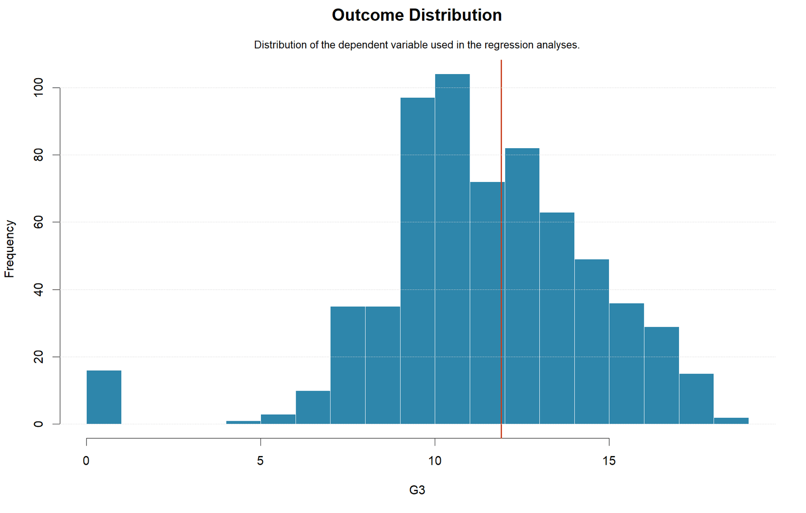
G3 Outcome Distribution
The chart shows a bounded, discrete grade outcome with a dense central mass and a visible lower tail. The complete model frame contains 649 observations. This structure helps explain why residual normality is imperfect even though the sample is large.
Statistical meaning: the outcome itself need not be normally distributed for ordinary least squares, but boundaries and discrete concentrations can generate asymmetric or heavy-tailed residual behavior.
nrow(model.frame(multiple_fit)) and verify that the chart uses the same G3 vector as the fitted objects.Simple lm Scatter and Line
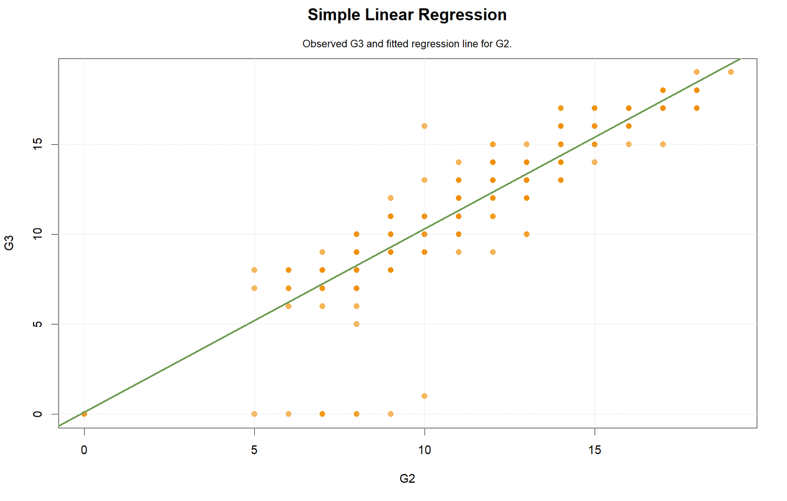
The points form a strong increasing pattern. The verified G2 slope is 1.0184903428 and simple R² is 0.8437304348. The line captures the dominant grade continuity while individual points remain above and below the fitted mean.
Statistical meaning: this is a bivariate sample association. It does not adjust for G1 or the other six variables and does not establish a causal effect of changing G2.
simple_fit, not the multiple fitted values, and reconcile the plotted equation with coef(simple_fit).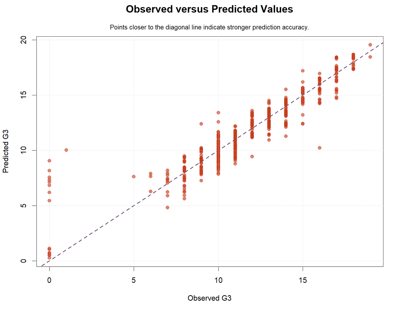
Observed Versus Fitted Values
The strong diagonal agreement corresponds to multiple R² = 0.8507771982. Fitted RMSE remains 1.2470202300, so the chart contains meaningful vertical errors even though the dense center looks close to the reference line.
Statistical meaning: high fitted agreement describes the current 649 observations. Boundary outcomes and unusual cases can still have large errors, and no unseen-data claim follows automatically.
fitted(multiple_fit), the y coordinates from model.response(model.frame(multiple_fit)), and confirm exactly 649 pairs.Residuals Versus Fitted
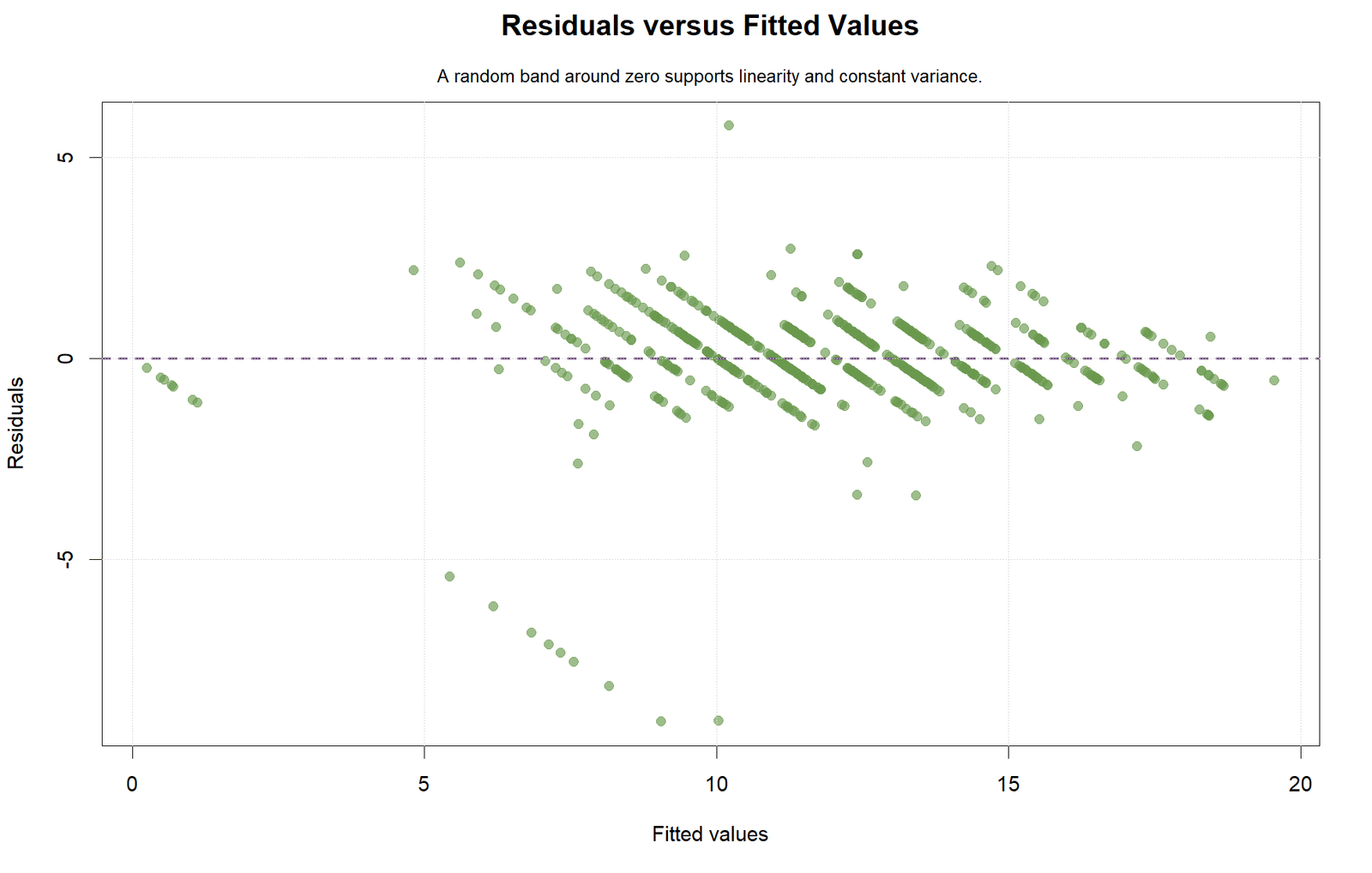
The residual cloud should be read with Breusch-Pagan = 35.7228073 and p = 1.9735 × 10⁻⁵. Changing spread or structured bands indicate that constant-variance classical uncertainty is doubtful.
Statistical meaning: a centered plot supports the mean equation only partially. It does not override a variance test, establish independence or guarantee normal tails.
residuals(multiple_fit) rather than standardized values labeled as raw residuals.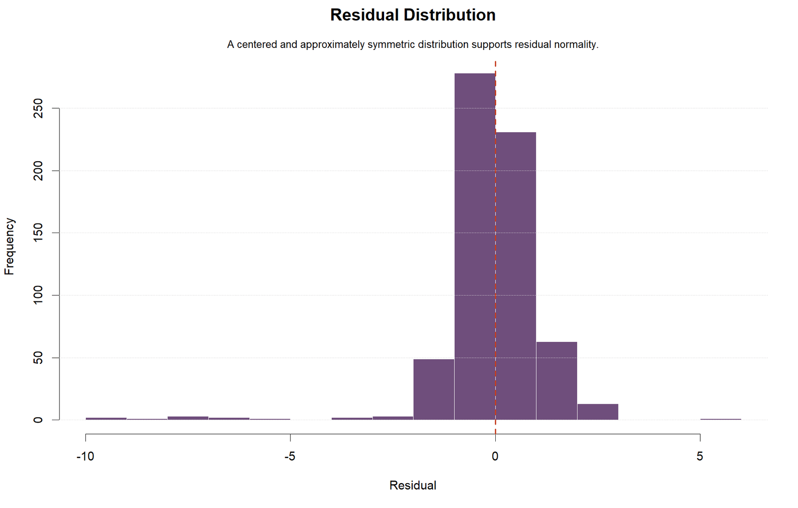
Residual Histogram
The main residual mass lies near zero, but the tails are not well represented by a symmetric normal shape. Shapiro-Wilk W = 0.7567934299 and Jarque-Bera = 9923.741889 reinforce the visual warning.
Statistical meaning: non-normal residuals affect classical reference inference more directly than the existence of the OLS coefficient estimates. With 649 rows, inspect tail influence and variance structure rather than treating one test as an automatic rejection of every model use.
residuals(multiple_fit) and report the same residual vector used by the tests.Normal Q-Q Plot
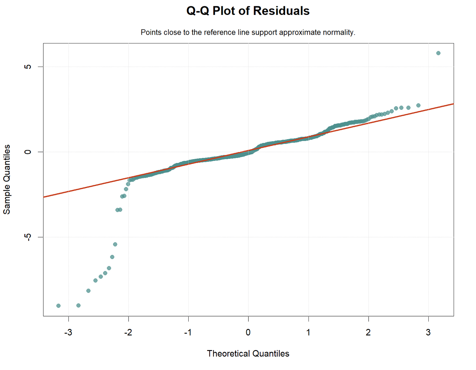
The central quantiles can align more closely than the tails, while pronounced end departures show where the normal reference fails. The chart should therefore be read together with case influence rather than summarized only as pass or fail.
Statistical meaning: tail departures may reflect bounded G3 values, unusual records, omitted structure or heterogeneous variance. A transformation or alternative specification should be justified by the research goal, not chosen mechanically.
qqnorm(residuals(multiple_fit)) and qqline(), preserving the same residual order and sample.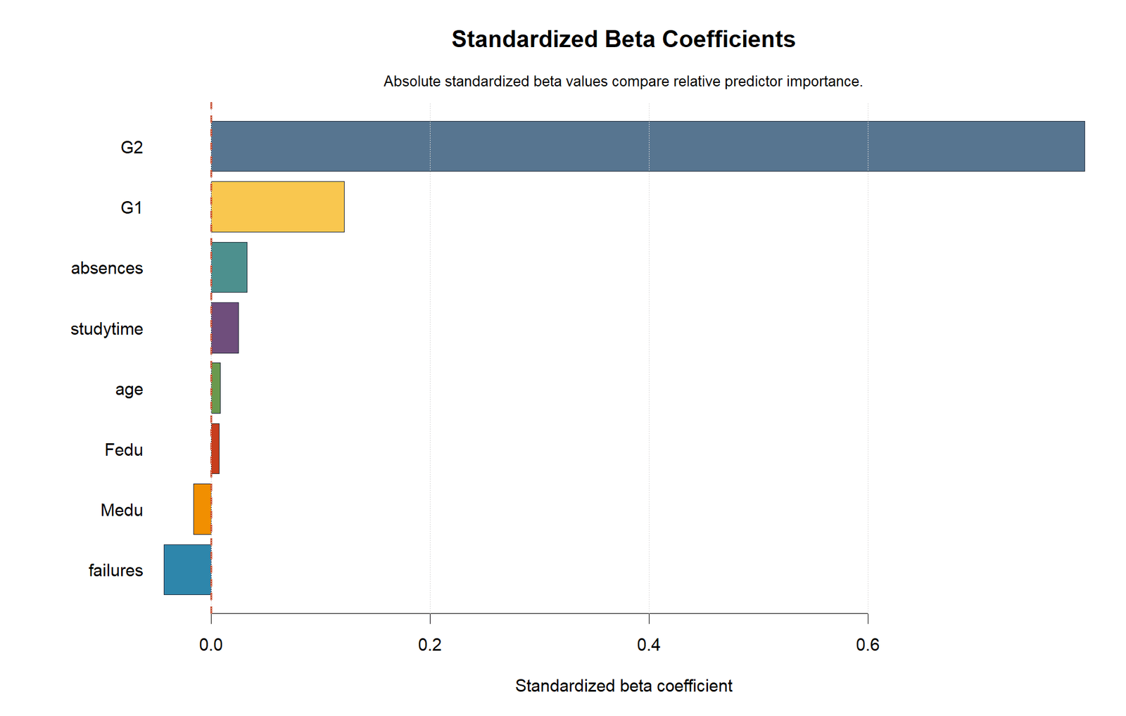
Standardized Beta Coefficients
G2 dominates with β = 0.7979830679, followed by G1 with β = 0.1218519798. Failures is −0.043219, absences is 0.032697 and the remaining absolute standardized values are small.
Statistical meaning: standardized beta compares slopes in sample standard-deviation units. It does not represent causal importance, and it remains sensitive to predictor overlap and sample variation.
Simple Versus Multiple Fit
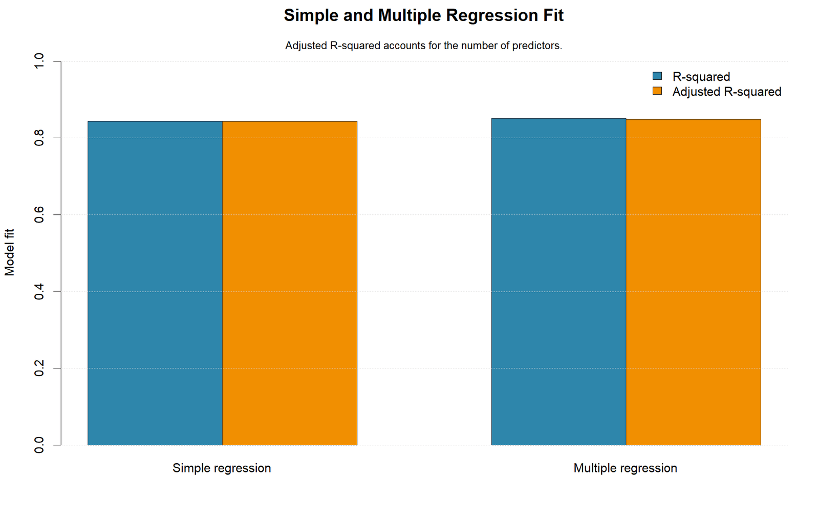
The multiple formula raises R² from 0.8437304348 to 0.8507771982 and lowers fitted RMSE from 1.2761246739 to 1.2470202300. The gain is real but modest.
Statistical meaning: G2 already provides a strong baseline. The additional predictors are most valuable for conditional interpretation and modest fitted refinement, not because adding variables always produces a materially better model.
Influence and Leverage
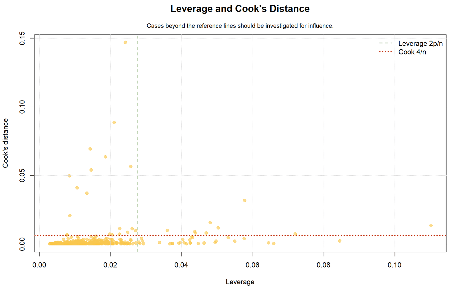
The figure locates observations with unusual predictor combinations, large residual impact or both. Leverage and Cook’s distance answer different questions, so one threshold should not be treated as an automatic deletion rule.
Statistical meaning: influential cases may be valid members of the target population. The correct response is source-data review, sensitivity refitting and disclosure of material changes.
hatvalues(), cooks.distance() and externally studentized residuals so every plotted point can be traced.Correlation Heatmap
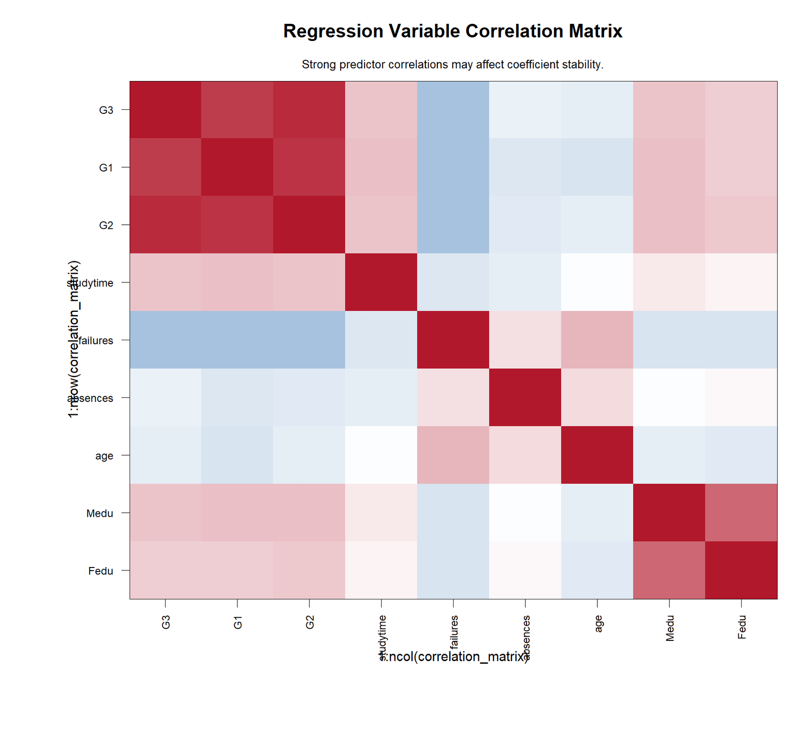
The strong G1-G2 relationship provides context for VIF = 4.1648316426 and 4.1207954322. Other predictors show less severe overlap.
Statistical meaning: a heatmap describes zero-order pairs; the multiple coefficients are conditional on all remaining columns. The two forms of evidence should explain one another rather than be substituted.
Regression in R Coefficient Interpretation
Regression in R coefficient meaning depends on the complete simultaneous predictor set.
Regression in R reports original-unit coefficients through coef() and summary(). Each multiple-model slope is conditional on the other seven variables, so it should not be described as a raw relationship.
G2
G2 has B = 0.8848073756 and a saved 95% interval from 0.817317 to 0.952298. Among records with the same G1, studytime, failures, absences, age, Medu and Fedu, a one-point G2 difference is associated with an expected 0.884807-point G3 difference. Its standardized beta of 0.797983 is the largest in the model.
G1
G1 has B = 0.1433966633, p = 0.0001020384 and β = 0.1218519798. Its conditional slope is much smaller than the strong grade continuity seen in a zero-order relationship because G2 absorbs substantial overlapping information.
Failures
Failures has B = −0.2353612027 and an interval excluding zero. At fixed values of the other predictors, an additional previous failure is associated with a lower expected G3. The standardized magnitude is modest, so statistical evidence should not be confused with a large effect.
Absences
Absences has B = 0.0227620294 and a small positive interval excluding zero. This is an adjusted coefficient and can differ in sign from the unadjusted association because prior grades and failures share information with absences. It is not evidence that missing school improves performance.
Studytime, Age, Medu and Fedu
The saved 95% intervals for these terms include zero. The result does not prove that the corresponding population effects are exactly zero. It shows that the current formula, predictor overlap and classical standard-error calculation do not isolate precise nonzero conditional slopes at the selected confidence level.
Intercept
The intercept is −0.501155 with an interval from approximately −2.0209 to 1.0186. It describes the fitted mean when every predictor equals zero, a combination that may have little substantive meaning. The intercept remains necessary for fitted predictions unless a zero-intercept model is explicitly justified.
Predictions, Effects and Model Meaning
Regression in R predictions should be separated into fitted means, mean intervals and individual prediction intervals.
Regression in R separates fitted values, mean-response intervals and individual prediction intervals. These quantities answer different questions and should not share one generic label.
Fitted Values
fitted(multiple_fit) returns expected G3 values for the observations used to estimate the model. Comparing those values with the observed response produces the saved RMSE and MAE. These are in-sample diagnostics.
New-Data Predictions
predict(multiple_fit, newdata = new_profiles) applies the coefficient vector to rows whose columns and classes match the model frame. Factors must have compatible levels, and extrapolation beyond the training ranges should be flagged.
Confidence and Prediction Intervals
Mean-response interval
- Use
interval = "confidence". - Estimates uncertainty in the conditional mean.
- Narrower than an individual prediction interval.
- Does not describe the spread of a new student’s outcome.
Individual prediction interval
- Use
interval = "prediction". - Includes mean uncertainty and residual variation.
- Relevant to a new observation under the same model assumptions.
- Still does not replace external validation.
Effects Versus Associations
The fitted slopes are conditional associations under the specified equation. The R object cannot establish that intervening on G2, failures or absences would produce the coefficient-sized change in G3. Causal claims require assumptions about assignment, confounding, measurement and study design beyond lm().
In-Sample Error Versus Generalization
Fitted RMSE = 1.2470202300 is calculated on the same observations that estimated the coefficients. A defensible predictive extension should split the data or perform resampling in a way that repeats every preprocessing and model-building step. The verified object should remain the baseline for comparison.
Regression in R Assumptions and Diagnostics
Regression in R diagnostics are decisions about separate assumptions, not one global pass-or-fail score.
Regression in R diagnostics answer separate questions. No single chart or p value certifies the complete model. The saved results should be read as a connected review of mean form, variance, residual shape, dependence, collinearity and case influence.
Linearity of the Conditional Mean
Inspect residuals against fitted values and against important predictors. Curvature or systematic structure suggests that the additive linear formula is incomplete. Candidate transformations or interactions should be justified substantively and compared with the verified baseline on the same observations.
Residual Variance
Breusch-Pagan = 35.7228073187 with p = 1.9734996372 × 10⁻⁵ provides evidence against constant residual variance under the test specification. Conventional OLS coefficients remain the least-squares estimates, but their classical standard errors may not describe uncertainty well.
Possible follow-up includes HC3 sandwich covariance, a modeled variance structure or an alternative response specification. The robust table should be labeled separately because it changes uncertainty estimates rather than silently replacing the fitted coefficient values.
Residual Normality
Shapiro-Wilk W = 0.7567934299 with p = 7.9184685958 × 10⁻³⁰ and Jarque-Bera = 9923.7418890 show strong departure from a normal residual reference. With 649 observations, inspect why the departure occurs: bounded outcome, tail cases, variance changes or mean misspecification.
Normal residuals are not required for the arithmetic existence of OLS estimates. The issue concerns classical finite-sample reference inference and whether the fitted equation adequately describes the data-generating structure.
Independence and Durbin-Watson
Durbin-Watson = 1.8615352810 is near the reference value two. However, the interpretation requires a meaningful row sequence. If rows are arbitrary, the statistic does not establish independence. If observations are clustered by school, class, family or repeated measurement, a different covariance or model structure may be needed.
Multicollinearity
G1 VIF = 4.1648316426 and G2 VIF = 4.1207954322 show substantial overlap between prior-grade variables. Their tolerances are about 0.240106 and 0.242672. These values warn that conditional coefficients may be less stable than zero-order associations, but they do not create a universal requirement to remove either variable.
Influence and Leverage
Review leverage, Cook’s distance, studentized residuals and DFFITS together. A high-leverage observation can have limited residual error, while a large residual at ordinary leverage can still matter. Connect every flagged index to the original record and compare refitted conclusions before making a decision.
Diagnostic Decision Table
| Evidence | Question | Appropriate next action | Incorrect shortcut |
|---|---|---|---|
| Residual-versus-fitted pattern | Is the conditional mean or variance structure incomplete? | Inspect curvature, spread, predictors and alternative specifications. | Declare the model valid because residuals average zero. |
| Shapiro-Wilk and Q-Q tails | Are residual-reference tails compatible with normal inference? | Review tail cases, robust inference and model form. | Delete observations until the p value exceeds .05. |
| Breusch-Pagan | Is variance approximately constant? | Report the warning and examine robust or modeled variance. | Ignore the result because R² is high. |
| VIF and tolerance | How much predictor information overlaps? | Discuss stability, theory and sensitivity. | Remove every variable above one arbitrary cutoff. |
| Cook’s distance and leverage | Which rows can materially affect the fit? | Trace records and conduct sensitivity refits. | Automatically delete every flagged case. |
| Fitted RMSE | How large are errors on the training rows? | Report as in-sample and add validation for prediction. | Rename it future test error. |
Regression in R Procedures and Reproducibility
Regression in R reproducibility requires a clean-session rerun and matching exported artifacts.
Regression in R becomes reproducible when the data preparation, object creation, diagnostics and exports are scripted in one ordered workflow.
Base fitting functions
read.csv()for declared importcomplete.cases()for one model framelm()for the fitted objectssummary()andanova()for core outputconfint()for coefficient intervals
Object audit functions
formula()model.frame()model.matrix()nobs()terms()andcontrasts()
Prediction and case audit
fitted()andresiduals()predict()hatvalues()cooks.distance()rstudent()
Optional diagnostic extensions
car::vif()lmtest::bptest()lmtest::dwtest()sandwich::vcovHC()lmtest::coeftest()
Recommended Run Order
- Set the topic folder and import the dataset with declared separators and column names.
- Inspect dimensions, names, classes, missing values and plausible ranges.
- Select G3 and the eight predictors into one complete-case frame.
- Confirm 649 rows and preserve row identifiers.
- Fit the simple and multiple objects.
- Verify formulas, model frames, design matrices and residual degrees of freedom.
- Export model comparison, coefficients, intervals and standardized betas.
- Export predictions, residuals, leverage and influence measures.
- Run residual-shape, variance, collinearity and dependence diagnostics.
- Create the ten charts from the same fitted objects and tables.
- Save full-precision CSV files and the report.
- Record
sessionInfo()and rerun from a clean session.
Reconciliation Checks
length(fitted(multiple_fit))must equal 649.df.residual(multiple_fit)must equal 640.- The coefficient table must contain one intercept and eight slopes.
- Residuals must equal the model response minus fitted values.
- RMSE must be computed from the same residual vector used in the charts.
- Standardized betas must use standard deviations from the model frame.
- VIF must be calculated from the same right-hand-side design.
- Chart titles and filenames must identify the correct object.
- Rounded article values must trace to full-precision exports.
R Code: Fit, Audit, Diagnose and Export
Regression in R code panels make the full object audit available without introducing another software workflow.
Regression in R code below keeps the analysis R-only and object-centered. Paths can be adapted to the topic folder, but the formula, model-frame logic and output labels should remain explicit.
1. Import and construct one complete-case model frame
dat <- read.csv("dataset.csv", check.names = FALSE)

vars <- c(
  "G3", "G1", "G2", "studytime", "failures",
  "absences", "age", "Medu", "Fedu"
)

stopifnot(all(vars %in% names(dat)))

model_dat <- dat[complete.cases(dat[vars]), vars]
stopifnot(nrow(model_dat) == 649L)

str(model_dat)
summary(model_dat)
colSums(is.na(model_dat))
This block prevents the simple and multiple formulas from selecting different observations.
2. Fit the simple and multiple lm objects
simple_fit <- lm(
  G3 ~ G2,
  data = model_dat
)

multiple_fit <- lm(
  G3 ~ G1 + G2 + studytime + failures +
    absences + age + Medu + Fedu,
  data = model_dat
)

formula(simple_fit)
formula(multiple_fit)
nobs(simple_fit)
nobs(multiple_fit)
df.residual(multiple_fit)
The verified multiple object should return 649 observations and 640 residual degrees of freedom.
3. Inspect the model frame and design matrix
mf <- model.frame(multiple_fit)
X  <- model.matrix(multiple_fit)
y  <- model.response(mf)

stopifnot(nrow(mf) == 649L)
stopifnot(nrow(X) == length(y))
stopifnot(colnames(X)[1] == "(Intercept)")

head(mf)
head(X)
attr(terms(multiple_fit), "term.labels")
Use this audit whenever classes, factors, transformations or interactions are possible.
4. Export summaries, ANOVA and confidence intervals
simple_summary   <- summary(simple_fit)
multiple_summary <- summary(multiple_fit)

coef_table <- as.data.frame(multiple_summary$coefficients)
coef_table$term <- rownames(coef_table)
rownames(coef_table) <- NULL

ci_table <- as.data.frame(confint(multiple_fit))
ci_table$term <- rownames(ci_table)
rownames(ci_table) <- NULL

anova_table <- as.data.frame(anova(multiple_fit))
anova_table$term <- rownames(anova_table)
rownames(anova_table) <- NULL

write.csv(coef_table, "multiple_coefficients.csv", row.names = FALSE)
write.csv(ci_table, "multiple_confidence_intervals.csv", row.names = FALSE)
write.csv(anova_table, "multiple_anova.csv", row.names = FALSE)
Full precision should remain in exported files even when the article rounds results.
5. Calculate model comparison and fitted error
model_metrics <- function(fit, name) {
  s <- summary(fit)
  e <- residuals(fit)

  data.frame(
    model = name,
    n = nobs(fit),
    r_squared = s$r.squared,
    adjusted_r_squared = s$adj.r.squared,
    f_statistic = unname(s$fstatistic[1]),
    df_model = unname(s$fstatistic[2]),
    df_residual = unname(s$fstatistic[3]),
    rmse = sqrt(mean(e^2)),
    mae = mean(abs(e)),
    residual_standard_error = s$sigma
  )
}

comparison <- rbind(
  model_metrics(simple_fit, "G3 ~ G2"),
  model_metrics(multiple_fit, "Eight-predictor model")
)

write.csv(comparison, "model_comparison.csv", row.names = FALSE)
RMSE uses an n denominator, while residual standard error uses residual degrees of freedom.
6. Calculate standardized beta coefficients
mf <- model.frame(multiple_fit)
response_sd <- sd(model.response(mf))

predictor_names <- names(mf)[-1]
predictor_sd <- vapply(mf[predictor_names], sd, numeric(1))

beta <- coef(multiple_fit)[predictor_names] *
  predictor_sd / response_sd

standardized_table <- data.frame(
  predictor = predictor_names,
  coefficient = coef(multiple_fit)[predictor_names],
  standardized_beta = unname(beta),
  row.names = NULL
)

write.csv(
  standardized_table,
  "multiple_standardized_betas.csv",
  row.names = FALSE
)
This direct formula is appropriate for the numeric predictor set used in the verified object.
7. Calculate VIF and tolerance
# Package-based calculation
vif_values <- car::vif(multiple_fit)

vif_table <- data.frame(
  predictor = names(vif_values),
  vif = as.numeric(vif_values),
  tolerance = 1 / as.numeric(vif_values)
)

write.csv(vif_table, "multiple_vif_tolerance.csv", row.names = FALSE)
Calculate VIF from the multiple object and exclude the intercept from substantive interpretation. Record the package version in the saved session information.
8. Export predictions, residuals and influence measures
case_audit <- transform(
  model.frame(multiple_fit),
  fitted = fitted(multiple_fit),
  residual = residuals(multiple_fit),
  standardized_residual = rstandard(multiple_fit),
  studentized_residual = rstudent(multiple_fit),
  leverage = hatvalues(multiple_fit),
  cooks_distance = cooks.distance(multiple_fit),
  dffits = dffits(multiple_fit)
)

case_audit$case_id <- rownames(model.frame(multiple_fit))
rownames(case_audit) <- NULL

write.csv(
  case_audit,
  "multiple_predictions_residuals_influence.csv",
  row.names = FALSE
)
Case identifiers are necessary for tracing every flagged point back to the source record.
9. Run residual diagnostics
e <- residuals(multiple_fit)

shapiro_result <- shapiro.test(e)
bp_result <- lmtest::bptest(multiple_fit)
dw_result <- lmtest::dwtest(multiple_fit)

diagnostic_table <- data.frame(
  diagnostic = c(
    "Shapiro-Wilk",
    "Breusch-Pagan",
    "Durbin-Watson"
  ),
  statistic = c(
    unname(shapiro_result$statistic),
    unname(bp_result$statistic),
    unname(dw_result$statistic)
  ),
  p_value = c(
    shapiro_result$p.value,
    bp_result$p.value,
    dw_result$p.value
  )
)

write.csv(
  diagnostic_table,
  "multiple_diagnostic_tests.csv",
  row.names = FALSE
)
The meaning of Durbin-Watson depends on the observation sequence; report row-order context.
10. Add an HC3 uncertainty sensitivity analysis
hc3_table <- lmtest::coeftest(
  multiple_fit,
  vcov. = sandwich::vcovHC(multiple_fit, type = "HC3")
)

hc3_export <- as.data.frame(hc3_table)
hc3_export$term <- rownames(hc3_export)
rownames(hc3_export) <- NULL

write.csv(
  hc3_export,
  "multiple_coefficients_hc3.csv",
  row.names = FALSE
)
Label this as a robust standard-error sensitivity analysis. It changes uncertainty estimates, not the fitted OLS coefficient values.
11. Create core base-R diagnostic charts
png("03_multiple_observed_vs_fitted.png", 2600, 1800, res = 300)
plot(
  fitted(multiple_fit),
  model.response(model.frame(multiple_fit)),
  xlab = "Fitted G3",
  ylab = "Observed G3",
  main = "Observed Versus Fitted"
)
abline(0, 1, lwd = 2)
grid()
dev.off()

png("04_multiple_residuals_vs_fitted.png", 2600, 1800, res = 300)
plot(
  fitted(multiple_fit),
  residuals(multiple_fit),
  xlab = "Fitted G3",
  ylab = "Residual",
  main = "Residuals Versus Fitted"
)
abline(h = 0, lwd = 2)
grid()
dev.off()

png("06_multiple_residual_qq.png", 2600, 1800, res = 300)
qqnorm(residuals(multiple_fit), main = "Normal Q-Q Plot")
qqline(residuals(multiple_fit), lwd = 2)
grid()
dev.off()
Each chart must use the verified multiple object and be exported with an unambiguous filename.
12. Save session information and the fitted objects
capture.output(
  sessionInfo(),
  file = "R_session_info.txt"
)

saveRDS(simple_fit, "simple_lm_object.rds")
saveRDS(multiple_fit, "multiple_lm_object.rds")
Saving the objects supports later auditing, but the script and data-preparation record are still required.
Advanced Regression in R Topics
Regression in R extensions should reproduce the verified baseline before claiming improvement.
Regression in R becomes more defensible when formula behavior, robust uncertainty, collinearity, influence, validation and software-state issues are handled explicitly.
Formula Environments and Data Masking
A formula can find variables in its environment when a name is absent from the supplied data. This flexibility can create hidden dependencies. Keep all modeled columns inside the declared data frame and inspect environment(formula(fit)) when reproducibility is critical.
Factors and Contrasts
A factor with several levels expands into contrast columns. The coefficient labels and interpretation depend on the contrast system and reference level. Save contrasts(), report the reference category and inspect model.matrix() before describing the slopes.
Ordered Variables Treated as Numeric
studytime, Medu and Fedu are coded as ordered numeric values in the verified equation. That treatment assumes a one-unit linear step. A factor treatment would estimate category contrasts instead. The choice should reflect the substantive question rather than convenience.
Sequential ANOVA Versus Overall Model Evidence
anova(multiple_fit) normally provides sequential sums of squares, so term order can affect individual rows when predictors overlap. The overall F statistic from summary() tests the complete slope block. Do not treat each sequential ANOVA row as identical to the corresponding coefficient t test.
Robust Standard Errors
The significant Breusch-Pagan result supports an HC3 sensitivity analysis. Report conventional and robust uncertainty separately, note the covariance estimator, and verify whether substantive conclusions change. Robust covariance does not repair nonlinearity, omitted variables, dependence or an inappropriate outcome model.
Prediction Intervals Under Heteroscedasticity
Classical predict.lm intervals inherit the fitted variance assumptions. When variance changes across fitted values, nominal interval coverage may be unreliable. A robust coefficient table alone does not automatically create robust individual prediction intervals.
VIF and Predictor Necessity
G1 and G2 have VIF values near four because both measure earlier achievement. Removing one may reduce collinearity but change the estimand and prediction content. Compare theoretically motivated formulas rather than applying a mechanical threshold.
Durbin-Watson and Row Order
Durbin-Watson 1.861535 is interpretable only when adjacent rows represent meaningful sequence. If the data are not time ordered, describe the value cautiously. If clustering is present, consider a model that represents that dependence instead of relying on row-order diagnostics.
Influence Sensitivity
Flagged rows should be reviewed for data errors, population relevance and structural uniqueness. Refit the equation with and without influential cases, compare coefficients and fitted conclusions, and report whether the central interpretation depends on a small number of observations.
Outcome Bounds
G3 is bounded and discrete. Ordinary least squares can still provide a useful conditional-mean baseline, but predicted values may extend beyond feasible limits and residual tails may be non-normal. Consider whether a transformed or alternative outcome model better matches the scientific goal, while retaining the verified lm result as a benchmark.
Validation and Resampling
Cross-validation or a holdout set is required for an honest predictive-error estimate. Every preprocessing decision, transformation and model selection step must occur inside the resampling loop. Otherwise information leakage makes the reported performance optimistic.
Rounding and Full Precision
Use rounded values in prose for readability, but retain full precision in CSV files and calculations. Recomputing a prediction or standardized beta from rounded coefficients can create small discrepancies that are not software errors.
Common Regression in R Mistakes
Object and coding mistakes
- Fitting candidate models on different complete-case samples.
- Allowing imported character codes to change numeric classes.
- Ignoring factor contrasts and reference levels.
- Creating plots from a different object than the tables.
- Calculating standardized beta from the full dataset rather than the model frame.
- Using row indices without preserving source identifiers.
Interpretation mistakes
- Calling a conditional slope a causal effect.
- Calling fitted RMSE future accuracy.
- Assuming high R² eliminates diagnostic concerns.
- Deleting predictors from VIF alone.
- Deleting cases from Cook’s distance alone.
- Treating a normality p value as the complete model decision.
Regression in R Decision Rules
- Write and report the formula before interpreting output.
- Use one 649-row model frame for the verified comparison.
- Inspect classes, contrasts and design-matrix columns.
- Report unstandardized B and confidence intervals as the main coefficient evidence.
- Use standardized beta as a supplementary within-sample comparison.
- Report Breusch-Pagan and residual-tail warnings.
- Trace influence points to source records before sensitivity refitting.
- Keep robust or transformed analyses separate from the baseline object.
- Use validation before making future-performance claims.
- Save full-precision tables, object files and session information.
- Regression in R should preserve one complete-case frame across model comparisons.
- Regression in R should identify every formula term and class.
- Regression in R should obtain charts and tables from the same fitted objects.
- Regression in R should retain full precision in exported data.
- Regression in R should report residual variance and tail evidence.
- Regression in R should distinguish fitted error from validation error.
- Regression in R should preserve row identifiers in influence audits.
- Regression in R should document package versions for diagnostic extensions.
- Regression in R should label robust covariance results separately.
- Regression in R should keep causal language within the design evidence.
APA-Style Reporting
Regression in R reporting should preserve diagnostic cautions beside the headline fit.
Regression in R reporting should identify the formula, sample, model fit, coefficient evidence, diagnostics and inferential limitations.
When robust standard errors or a validation analysis are added, state the covariance estimator or resampling design explicitly and do not merge those results silently with the classical summary.lm table.
Publication Checklist
Regression in R publication checks protect both numerical accuracy and interpretation.
Regression in R should pass the following checks before the post and downloadable report are released.
- State G3 as the outcome and list all eight multiple predictors.
- Report the exact simple and multiple formulas.
- Confirm the same 649 observations are used in both objects.
- Report R², adjusted R², fitted RMSE and residual standard error accurately.
- Report the overall F statistic with eight and 640 degrees of freedom.
- Report B, interval and standardized beta with matching term labels.
- Explain that G2 dominates the fitted standardized comparison.
- Interpret the positive absences coefficient as conditional, not causal.
- Report Shapiro-Wilk, Jarque-Bera and Breusch-Pagan warnings.
- Explain the row-order limitation of Durbin-Watson.
- Report G1 and G2 VIF values with context rather than a mechanical deletion rule.
- Verify that all ten charts come from the correct R objects.
- Verify every chart URL, caption and alternative text.
- Retain full precision in the report or result tables.
- Label fitted error as in-sample.
- Preserve all advertisement placements and the back-to-top control.
Downloads and R Chart Resources
Regression in R resources below are tied directly to the verified R analysis.
Regression in R downloads are limited to the verified R report and the ten R-generated chart assets used in the article.
01 Outcome distributionG3 distribution for the verified model frame
02 Simple regression lineG2 versus G3 with the simple lm fit
03 Observed versus fittedMultiple-object fitted agreement
04 Residuals versus fittedMean-form and variance diagnostic
05 Residual histogramShape and tail review
06 Residual Q-Q plotNormal-reference quantile comparison
07 Standardized betasWithin-model standardized effect comparison
08 Model-fit comparisonSimple and multiple fitted metrics
09 Influence diagnosticsLeverage and case-impact review
10 Correlation heatmapPairwise structure among modeled variables
Frequently Asked Questions
Regression in R answers below retain the limits of the saved analysis.
Regression in R questions below focus on the choices most likely to change the fitted object or its interpretation.
Which R function fits the verified models?
The workflow uses lm() with explicit formulas: G3 ~ G2 and the eight-predictor multiple formula.
Why should model.frame be checked?
It reveals the exact evaluated variables and rows used by the object. This prevents descriptive tables, charts or candidate fits from silently using a different sample.
Why must the simple and multiple models use the same rows?
Otherwise changes in R², RMSE or coefficients can reflect missing-data differences rather than the predictor formula.
What is the difference between RMSE and residual standard error?
Fitted RMSE is the square root of the mean squared case residual using n in the denominator. Residual standard error uses residual degrees of freedom. They are related but not identical.
Why is G2 the strongest predictor?
Its standardized beta is 0.797983, much larger in absolute magnitude than the other saved coefficients. This conclusion applies to the verified sample and formula.
Why are G1 and G2 VIF values near four?
They are strongly related prior-grade measures. Their overlap affects conditional slope stability, but the values do not automatically require removing either term.
Does lm automatically validate assumptions?
No. It estimates the model. Mean form, variance, residual tails, independence, collinearity, influence and design validity require separate review.
Does the Shapiro-Wilk result invalidate every use of the model?
No. It provides strong evidence against a normal residual reference. The consequences depend on the inferential purpose, tail influence, variance structure and possible model misspecification.
What should be done after the significant Breusch-Pagan result?
Report the heteroscedasticity evidence, inspect the residual pattern, and consider HC3 uncertainty or a variance model. Do not imply that robust standard errors fix every specification problem.
Can influential observations be deleted automatically?
No. Trace them to source records, determine whether they are errors or valid cases, refit sensitivity models and report any material changes.
Can fitted RMSE be reported as future prediction error?
No. Future performance requires unseen observations or a correctly designed resampling procedure.
What should be saved for reproducibility?
Save the script, data-preparation rules, full-precision tables, charts, report, fitted objects and sessionInfo().
Why should robust results be labeled separately?
An HC3 table changes covariance and uncertainty estimates while retaining the same OLS slopes. Readers should be able to distinguish the classical baseline from the sensitivity analysis.
Regression in R Conclusion
Regression in R is strongest when the model object and the scientific claim remain aligned.
Regression in R verifies a strong eight-predictor fitted relationship for G3. The multiple object uses 649 rows, reports R² = 0.8507771982, adjusted R² = 0.8489119132 and F(8, 640) = 456.1110974, and identifies G2 as the dominant standardized predictor with β = 0.7979830679.
The result is not assumption-free. Residual normality tests show substantial tail departure, Breusch-Pagan indicates nonconstant variance, G1 and G2 overlap strongly, and influence review remains necessary. These findings support careful uncertainty analysis and sensitivity work rather than causal wording or guaranteed unseen-cohort performance.
The central strength of Regression in R is the object-centered audit trail: the formula defines the estimand, the model frame identifies the observations, the design matrix identifies the encoded columns, and the same fitted object generates coefficients, intervals, predictions, residuals, diagnostics, charts and exports.

