
Guttman’s Lambda-6: 7 Essential Steps, Formula and Worked Example
Guttman’s Lambda is a family of six lower-bound reliability coefficients. This guide focuses on Guttman’s Lambda-6, the regression-error coefficient that predicts every item from all remaining items, sums the unexplained item variances, and compares that error total with the variance of the composite score. The worked analysis uses six student questionnaire items, 649 complete cases, and independently matched Python, R, SPSS and Excel results.
Six items
649 complete cases
Regression-error method
Python + R + SPSS + Excel
The six-item composite has a low Guttman’s Lambda-6 of 0.288772.
For the 649 complete observations, the total score variance was 8.818552759. Predicting each item from the other five items produced a summed residual error variance of 6.272000531. Therefore, the lower-bound reliable variance was 2.546552229, and Guttman’s Lambda-6 = 1 – 6.272000531 / 8.818552759 = 0.288772126. In practical terms, the six selected variables do not function as a strongly coherent single composite in this dataset.
What does Guttman’s Lambda measure?
A lower bound for the reliability of a composite score, estimated from the covariance structure among its items.
Guttman’s Lambda refers to six coefficients introduced as lower bounds for the reliability of a sum of variables. The coefficients do not all use the same computational route. Some are based on item variances and covariances, one corresponds to coefficient alpha, one depends on a particular split of the test, and Guttman’s Lambda-6 uses squared multiple correlations to estimate how much of each item can be predicted from all the other items.
The reliability question
Suppose a researcher adds several items to create one total score. The observed total varies because people differ on the intended construct, because the items may capture other systematic dimensions, and because measurement error and item-specific variance remain. A reliability coefficient summarizes how consistently the item set behaves as a composite under a stated model. Guttman’s Lambda-6 asks how much error remains after the linear information in the other items is used to predict each item.
For item j, the remaining items form a multiple regression model. The model’s squared multiple correlation, Rj2, is the proportion of that item’s variance linearly predictable from the rest of the scale. The residual proportion, 1 – Rj2, is multiplied by the item’s variance. Those residual variances are then summed and divided by total-score variance.
What Lambda-6 does not establish
A high Guttman’s Lambda coefficient does not prove that all items measure one factor, that the scale is valid for its intended interpretation, or that scores are unbiased. Lambda-6 is sensitive to the correlation structure, including clustered or “lumpy” groups of items. A multidimensional item set can sometimes produce a substantial coefficient because items are predictable within subclusters.
A low value is also not automatically a software failure. It may reflect heterogeneous content, weak inter-item relationships, inappropriate item direction, restricted response ranges, poorly chosen items, or a total score that should not have been formed. Reliability evidence must therefore be read alongside content validity, dimensionality, scoring logic and the intended use of scores.
The worked example demonstrates why this distinction matters. The selected variables describe family relationships, free time, going out, reverse-coded alcohol consumption and health. They can be added numerically, but their content is broad. The resulting Guttman’s Lambda-6 of 0.288772 signals that the sum should not be treated as a dependable one-dimensional score without stronger theoretical and empirical justification.
When should you use Guttman’s Lambda-6?
Use it as part of a reliability study when a multi-item total or average score has a defensible measurement purpose.
Use Guttman’s Lambda-6 when the research problem concerns the dependability of a composite score and the analyst wants an error estimate based on each item’s linear predictability from the other items. It is especially informative when item loadings or item relationships are unequal, because the coefficient does not require the same tau-equivalence logic commonly associated with a strict reading of coefficient alpha.
Define one score
State why the selected items should be summed or averaged and what the composite is intended to represent.
Check direction
Recode negatively oriented items so that high scores have a consistent substantive direction before forming the total.
Inspect structure
Review item distributions, correlations, corrected item-total relationships and evidence about dimensionality.
Calculate Lambda-6
Regress each item on the remaining items, obtain squared multiple correlations and sum residual variances.
Interpret in context
Compare the coefficient with the decision stakes, score use, item content and other reliability estimates.
Appropriate applications
Guttman’s Lambda can support analyses of survey scales, educational tests, rating composites, behavioral indices and multi-item assessments when respondents or observational units are independent and the total score has a clear meaning. It can be reported with coefficient alpha, omega and item diagnostics rather than as a stand-alone certificate of quality.
Exploratory scale review
Lambda-6 can help identify whether items contain useful shared linear information. The item-level R2 values show which variables are well predicted by the remaining set and which behave mostly as unique variables. This makes the method useful during scale refinement, although item deletion should never be driven by one number alone.
Unsuitable uses
Do not use Guttman’s Lambda-6 for a single item, unrelated variables assembled only because they share a dataset, nominal variables without meaningful numerical scoring, repeated measurements where temporal stability is the target, or inter-rater agreement. Those designs require different reliability or agreement methods.
Search-intent clarification
Searches such as Guttmans lambda, Guttmans lambda 6, Guttmans 6 lambda and Guttmans lambda 2 usually refer to the six lower-bound reliability coefficients. The apostrophe is often omitted in search queries, but the statistical name is normally written Guttman’s Lambda. Lambda-2 and Lambda-6 are related lower bounds, not version numbers of the same formula.
Guttman’s Lambda assumptions and data requirements
The coefficient is computationally direct, but meaningful interpretation depends on measurement design and data quality.
Guttman’s Lambda is sometimes described as assumption-free because it is not a normal-theory significance test. That description is misleading. The coefficient still depends on a coherent composite, independent observations, appropriate numerical scoring, linear item relationships, defensible missing-data handling and an interpretable covariance matrix.
1. A defensible composite score
The items must have a substantive reason to form one score. Reliability is a property of scores in a population and context, not an intrinsic label permanently attached to a questionnaire. If the items represent unrelated constructs, a low Guttman’s Lambda-6 is expected and should not be repaired merely by deleting inconvenient variables.
2. Consistent item direction
Items should be oriented so that high values have a compatible meaning. In the worked example, workday alcohol use and weekend alcohol use were transformed as Dalc_R = 6 – Dalc and Walc_R = 6 – Walc. A value of 5 on the reversed item therefore represents lower original alcohol consumption, while a value of 1 represents higher original consumption.
3. Independent observational units
The 649 rows are treated as separate students. Clustered classrooms, repeated measurements, family clusters or multilevel sampling can alter the covariance structure and the uncertainty of reliability estimates. A single coefficient calculated as though all rows were independent can conceal that design.
4. Linear predictability
Lambda-6 uses ordinary multiple regression logic. Each item is predicted by a linear combination of the remaining items. Strong nonlinear relationships may not be captured by the squared multiple correlation. Severe outliers can also affect variances, correlations and regression fits.
5. Adequate information and stable matrix
The sample must be large enough relative to the number of items for the item regressions and correlation matrix to be stable. Perfectly duplicated items, near-linear dependence or an ill-conditioned correlation matrix can produce unstable squared multiple correlations. With six items and 649 complete cases, the numerical regressions are well determined, although substantive coherence remains weak.
6. Transparent missing-data rule
SPSS used 649 valid cases and excluded zero cases. Python, R and Excel used the same complete rows. When missing values exist, listwise deletion, pairwise correlations, imputation and available-item scoring can produce different covariance matrices and therefore different Guttman’s Lambda values. The rule must be documented before results are compared.
Neither a high nor low Guttman’s Lambda-6 removes the need for dimensionality analysis. The coefficient does not test a one-factor model. Examine the correlation matrix, factor structure, item content and score purpose. In this example, the mean inter-item correlation is only 0.033 and several correlations are negative even after the two alcohol variables are reversed. That pattern is consistent with a broad, weakly unified item set.
Guttman’s Lambda-6 formula and seven-step calculation
Lambda-6 subtracts the proportion of total-score variance represented by the summed item residual variances.
The raw-score Guttman’s Lambda-6 formula uses the sample variance of each item, the squared multiple correlation from regressing that item on all other items, and the variance of the sum score. It is essential to include item variances when items are not standardized.
λ6 is Guttman’s Lambda-6; k is the number of items; sj2 is item j‘s variance; Rj2 is the squared multiple correlation when item j is regressed on all remaining items; and sX2 is the variance of the sum score X.
sj2Rj2 is the portion of an item’s variance linearly predicted by the other items.
sj2(1 – Rj2) is the portion not predicted by the remaining items.
sX2 – Σej2 is the variance retained after subtracting summed item residual variance.
Seven calculation steps
Guttman’s Lambda 1 through Lambda 6
SPSS reports six related lower bounds, and each coefficient reflects a different decomposition of error.
The phrase Guttman’s Lambda is singular in casual use, but the original family contains six lower bounds. A complete reliability analysis should identify which lambda is being reported. Guttman’s Lambda-2 and Guttman’s Lambda-6 are not interchangeable, while Lambda-3 is numerically equivalent to raw coefficient alpha.
| Coefficient | SPSS value | Core idea | Interpretive note for this example |
|---|---|---|---|
| Lambda-1 | 0.093 | Starts from the sum of item variances relative to total-score variance. | A very small lower bound because shared covariance is weak. |
| Lambda-2 | 0.294 | Adjusts Lambda-1 using the covariance information among items. | Slightly above Lambda-6 and a direct match for the search phrase “Guttmans lambda 2.” |
| Lambda-3 | 0.112 | Equivalent to Cronbach’s coefficient alpha for the raw item covariance matrix. | Confirms very low conventional internal consistency. |
| Lambda-4 | -0.312 | A split-half lower bound based on a specified division of items. | The selected split produced a negative value, indicating an incompatible half-score relationship. |
| Lambda-5 | 0.316 | Uses the largest row sum of squared covariances in its error adjustment. | The largest of the six SPSS lower bounds in this output, but still low. |
| Lambda-6 | 0.289 | Uses each item’s squared multiple correlation with all remaining items. | The exact independently calculated value is 0.288772126. |
Why can the six values differ?
Each lambda defines or bounds error differently. Lambda-6 treats the residual variance from a multiple regression as item-specific error for the lower-bound calculation. Lambda-4 depends on how items are divided into halves. Lambda-3 uses the alpha formula. When items have unequal correlations, subclusters or mixed directions, the coefficients can separate substantially.
The worked results range from -0.312 to 0.316. That range is not a contradiction. It is evidence that the item set is structurally weak and that some decompositions are especially unfavorable. Reporting only the largest coefficient without identifying it would overstate the clarity of the reliability evidence.
Should the largest lambda always be reported?
Guttman’s lower-bound framework motivates attention to the largest defensible lower bound, but applied reporting should remain transparent. State the coefficient, formula, software behavior and item set. If SPSS reports all six, present the pattern rather than hiding negative or small values.
For this example, Lambda-5 is the numerical maximum at 0.316, Lambda-2 is 0.294, and Lambda-6 is 0.289. All three lead to the same substantive conclusion: the six-variable total has limited internal consistency as a single score.
Guttman’s Lambda worked example: six student questionnaire items
The analysis uses the 649-case Portuguese-language student performance data and a deliberately transparent scoring transformation.
This Guttman’s Lambda example uses six five-point variables: quality of family relationships, free time after school, going out with friends, reversed workday alcohol consumption, reversed weekend alcohol consumption and current health. All 649 rows contain valid values for the selected variables.
| Analysis name | Meaning and coding | Mean | SD | Role in total |
|---|---|---|---|---|
| famrel | Quality of family relationships, 1 = very bad to 5 = excellent. | 3.9307 | 0.95572 | Higher values indicate more favorable family relationships. |
| freetime | Free time after school, 1 = very low to 5 = very high. | 3.1803 | 1.05109 | Higher values indicate more free time, not necessarily a better outcome. |
| goout | Going out with friends, 1 = very low to 5 = very high. | 3.1849 | 1.17577 | Higher values indicate more social outings. |
| Dalc_R | Reverse-scored workday alcohol use: Dalc_R = 6 – Dalc. | 4.4977 | 0.92483 | Higher values indicate lower original workday alcohol use. |
| Walc_R | Reverse-scored weekend alcohol use: Walc_R = 6 – Walc. | 3.7196 | 1.28438 | Higher values indicate lower original weekend alcohol use. |
| health | Current health status, 1 = very bad to 5 = very good. | 3.5362 | 1.44626 | Higher values indicate better self-reported health. |
Observed correlation pattern
The strongest positive correlation is between Dalc_R and Walc_R, r = 0.617, which is expected because workday and weekend drinking behaviors are related. Freetime and goout correlate r = 0.346. Goout is negatively correlated with Dalc_R (r = -0.245) and Walc_R (r = -0.389), meaning that greater social outings are associated with lower reverse-coded alcohol scores, or higher original alcohol use.
Most other relationships are small. Health correlates from -0.115 to 0.110 with the remaining variables. Famrel correlations range from 0.076 to 0.129. The overall mean inter-item correlation is only 0.033, so the covariance available to support one total score is limited.
Total-score descriptives
The six-item total has a mean of 22.0493, a sample variance of 8.818552759 and a standard deviation of 2.96960. The item variances are not equal, ranging from approximately 0.855 for Dalc_R to 2.092 for health. This is why the raw-score Lambda-6 calculation must multiply each residual proportion by its own item variance.
Because there are zero excluded cases, the same 649 observations contribute to all item regressions, the total-score variance and the SPSS Guttman model. This common analysis sample is a major reason the Python, R, SPSS and Excel results match.
Guttman’s Lambda-6 results and item-level interpretation
The exact coefficient is built from six squared multiple correlations and six residual variance components.
The Guttman’s Lambda-6 results show which items are predictable from the rest of the composite. Weekend alcohol use has the largest squared multiple correlation, while health and family relationships have very small values. Those low item R2 values leave substantial residual variance in the numerator of the formula.
| Item | Squared multiple correlation | Predicted item variance | Residual error variance | Result meaning |
|---|---|---|---|---|
| famrel | 0.053245 | 0.048634 | 0.864761 | Only 5.32% of family-relationship variance is predicted by the other five items. |
| freetime | 0.138326 | 0.152822 | 0.951973 | 13.83% is predicted; most variance remains item-specific. |
| goout | 0.257962 | 0.356613 | 1.025810 | 25.80% is predicted, mainly through relationships with free time and alcohol-use items. |
| Dalc_R | 0.382171 | 0.326878 | 0.528441 | 38.22% is predicted; this is one of the more integrated items. |
| Walc_R | 0.455906 | 0.752077 | 0.897555 | 45.59% is predicted, the highest item R2 in the set. |
| health | 0.042171 | 0.088208 | 2.003460 | Only 4.22% is predicted, and its high variance makes it the largest residual contributor. |
Final verified coefficient
Low internal consistency for one composite
The exact Python and Excel value is 0.28877212602212743; the R value differs only in printed decimal length. SPSS rounds the result to 0.289.
What drives the low value?
Health contributes 31.94% of the summed residual variance by itself. Goout contributes 16.36%, freetime 15.18%, Walc_R 14.31%, famrel 13.79% and Dalc_R 8.43%. Health is both highly variable and poorly predicted by the other items, so it strongly increases the Lambda-6 error numerator.
The coefficient would not be improved responsibly by deleting health solely because of this contribution. First ask whether health belongs in the intended construct. If it does, low reliability may indicate that the construct is broad or that additional related health items are needed. If it does not, the original total-score definition should be revised on conceptual grounds.
Guttman’s Lambda in Python: verified calculations and charts
The Python workflow independently reproduces each item regression, residual component and final Lambda-6 value.
A reliable Guttman’s Lambda Python workflow should not hard-code the final coefficient. It should build the total score, run one regression per item, obtain each squared multiple correlation, calculate residual item variance and then apply the raw-score Lambda-6 formula. The downloadable Python report records the exact calculation and five result graphics.
import pandas as pd
import statsmodels.api as smdf = pd.read_csv("dataset.csv")
items = df[["famrel", "freetime", "goout", "Dalc", "Walc", "health"]].copy()
items["Dalc"] = 6 - items["Dalc"]
items["Walc"] = 6 - items["Walc"]
items.columns = ["famrel", "freetime", "goout", "Dalc_R", "Walc_R", "health"]
items = items.dropna()
total_variance = items.sum(axis=1).var(ddof=1)
error_variances = []
for item in items.columns:
y = items[item]
X = sm.add_constant(items.drop(columns=item))
r_squared = sm.OLS(y, X).fit().rsquared
error_variances.append(y.var(ddof=1) * (1 - r_squared))
lambda_6 = 1 - sum(error_variances) / total_variance
print(lambda_6) # 0.288772126
Python chart 1: primary metrics
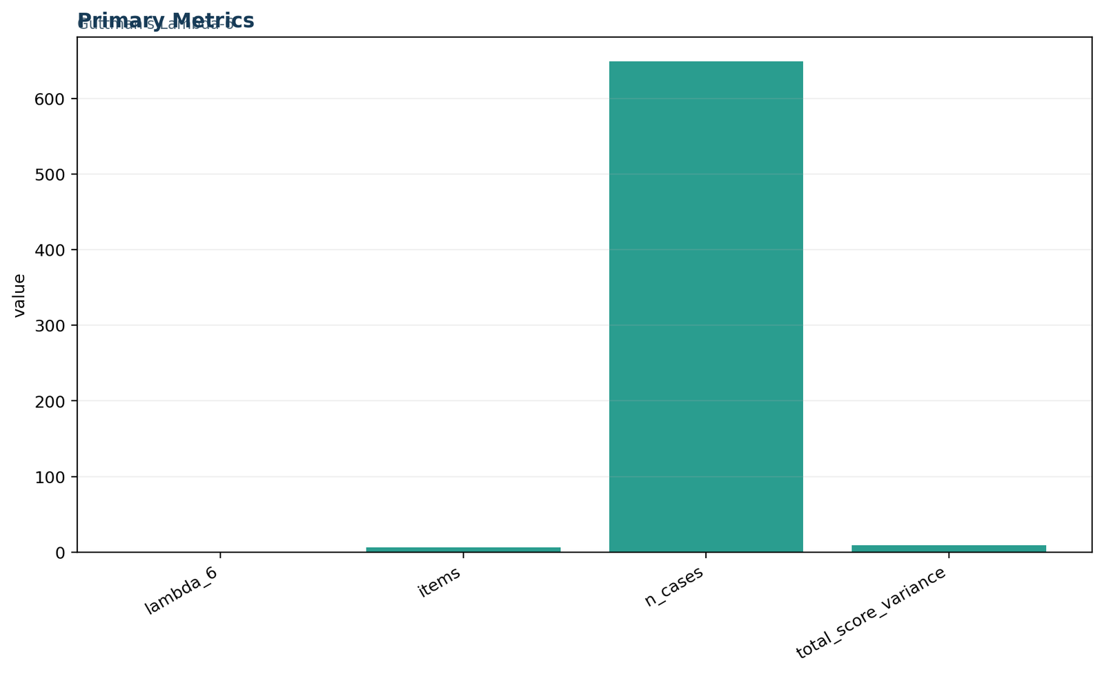
The first chart places the four headline values in one frame: Lambda-6 = 0.288772, six items, 649 cases and total-score variance = 8.818553. Because the metrics use very different scales, the 649-case bar dominates the visual height. The numerical values, rather than relative bar lengths, carry the main interpretation. This chart is best used as an audit summary confirming that the same dataset dimensions and variance entered the calculation.
Python chart 2: Lambda-6 item components
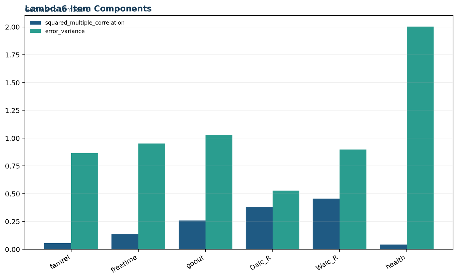
The paired bars compare each squared multiple correlation with its residual error variance. Walc_R has the highest R2 at 0.455906, followed by Dalc_R at 0.382171 and goout at 0.257962. Health has the lowest R2 at 0.042171 and the largest residual variance at 2.003460. The chart makes the central Lambda-6 mechanism visible: weak item predictability leaves a large error component.
Python chart 3: predicted item variance
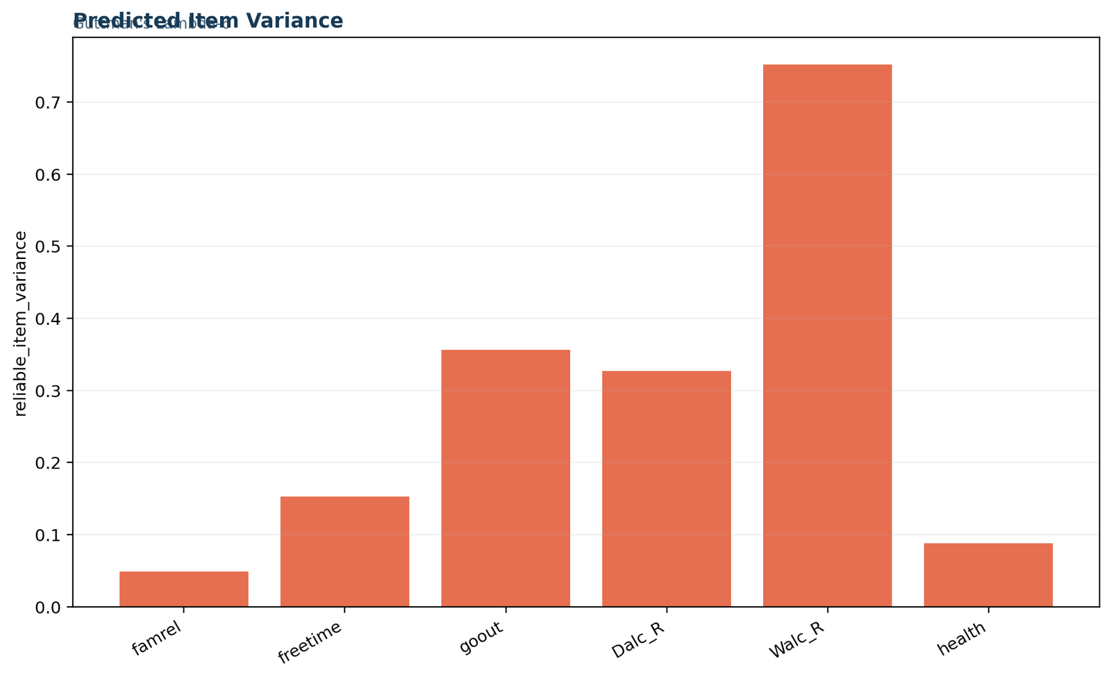
This chart isolates sj2Rj2, the part of each item’s variance predicted by the other items. Walc_R contributes 0.752077, far more than any other variable. Goout contributes 0.356613, Dalc_R 0.326878, freetime 0.152822, health 0.088208 and famrel 0.048634. These are not separate reliability coefficients; they are item-level components that help explain why the final Lambda-6 remains low.
Python chart 4: Lambda-6 result block
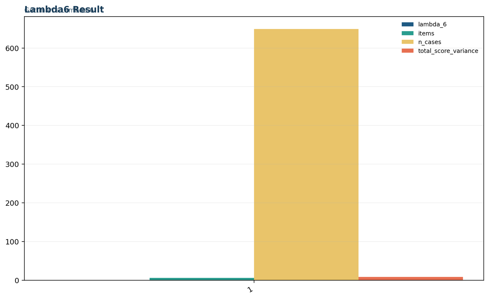
The result chart confirms the exact analysis ledger. Lambda-6 is 0.288772, the item count is 6, the sample size is 649 and total-score variance is 8.818553. The case count again controls the common scale, so the small reliability bar is visually compressed. The chart is a reproducibility check rather than an effect-size comparison.
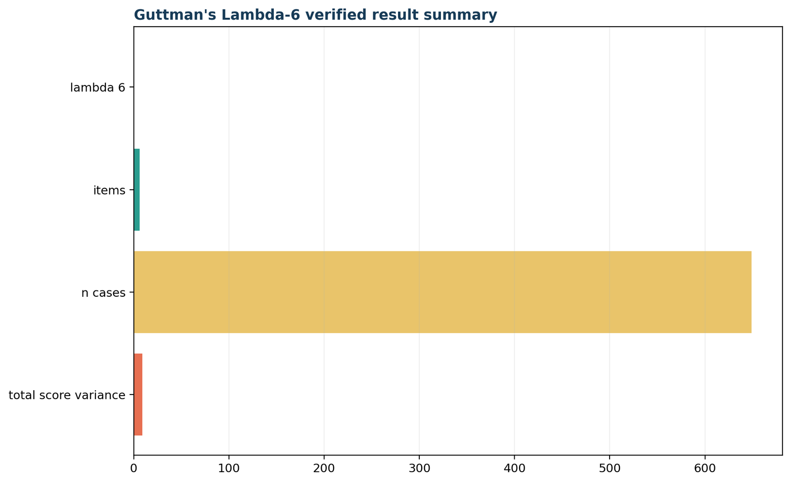
Python chart 5: verified result summary
The final horizontal summary repeats the independently verified outputs and is useful when reviewing the PDF report against SPSS and Excel. Agreement across artifacts is exact to floating-point precision: the only visible differences arise from rounding. The chart does not imply that all four metrics should be compared substantively on one axis.
Python calculation logic
For each item, the Python analysis designates that variable as the dependent variable and uses the other five as predictors. The model R2 becomes the squared multiple correlation. The sample variance of the dependent item is multiplied by 1 – R2. After all six residual components are added, the sum is divided by the sample variance of the row-wise total score.
This explicit method is preferable to relying on a package label when cross-software agreement matters. It also exposes whether a software implementation uses raw covariances, standardized items, population variances or sample variances.
Python verification checklist
Guttman’s Lambda in R: regression-error reliability and matched charts
The R report reproduces the same raw-score coefficient and verifies the result independently.
The Guttman’s Lambda R workflow can be implemented directly from the formula or obtained as G6(smc) in a broader reliability analysis. For exact cross-platform verification, the supplied R analysis uses the same six transformed items, the same complete cases, the same item-wise multiple regressions and the same sample total-score variance.
d <- read.csv("dataset.csv")

items <- data.frame(

famrel = d$famrel,

freetime = d$freetime,

goout = d$goout,

Dalc_R = 6 - d$Dalc,

Walc_R = 6 - d$Walc,

health = d$health

)

items <- na.omit(items)total_variance <- var(rowSums(items))

r2 <- sapply(names(items), function(item) {

predictors <- setdiff(names(items), item)

summary(lm(reformulate(predictors, response = item), data = items))$r.squared

})

error_variance <- sapply(names(items), function(item) var(items[[item]])) * (1 - r2)

lambda_6 <- 1 - sum(error_variance) / total_variance

lambda_6  # 0.288772126
R chart 1: primary metrics
The R primary-metrics chart confirms λ6 = 0.288772126022127, six items, 649 cases and total-score variance 8.81855275923072. The final decimal display is slightly shorter than Python because of report formatting, not a computational disagreement. The shared metric ledger is the first cross-check before item-level components are interpreted.
R chart 2: squared multiple correlations and residuals
The R item-components figure should reproduce the same six R2 values and error variances as Python. The strongest predictable pair of variables is represented by the reversed workday and weekend alcohol items. Health remains weakly connected to the rest, leaving the largest unexplained variance component and lowering Guttman’s Lambda-6.
R chart 3: variance predicted by the remaining items
The reliable-item-variance bars quantify the product of item variance and the squared multiple correlation. Walc_R contributes the most predicted variance at 0.752077. Famrel and health contribute very little despite being substantively meaningful variables, showing that importance to a research topic is not the same as integration within a particular composite score.
R chart 4: final Lambda-6 ledger
The result chart presents the coefficient with sample and scale dimensions. Its purpose is to make report-to-report reconciliation easy. If an R package returns a materially different result, check whether it calculated standardized G6 from a correlation matrix, used pairwise correlations, automatically imputed missing data or applied a different item-keying rule.
R chart 5: verified result summary
The final R summary closes the independent replication. R, Python and Excel agree on all reported metrics, and SPSS displays the same Lambda-6 rounded to three decimals. This agreement verifies the arithmetic; it does not change the substantive conclusion that the six items have weak internal consistency as one total.
Guttman’s Lambda in SPSS: menu, syntax and output interpretation
SPSS directly reports Lambda 1 through Lambda 6 through the Guttman reliability model.
To calculate Guttman’s Lambda in SPSS, open Analyze, choose Scale, select Reliability Analysis, move the intended items into the Items box and select Guttman as the model. The verified syntax uses the six transformed variables and requests descriptive, scale, correlation and total-item statistics.
COMPUTE Dalc_R=6-Dalc.

COMPUTE Walc_R=6-Walc.

EXECUTE.RELIABILITY

/VARIABLES=famrel freetime goout Dalc_R Walc_R health

/SCALE('Guttman reliability') ALL

/MODEL=GUTTMAN

/STATISTICS=DESCRIPTIVE SCALE CORR

/SUMMARY=TOTAL MEANS VARIANCE CORR.
Verified SPSS setup
The active dataset contains 649 rows. The analysis first creates Dalc_R = 6 – Dalc and Walc_R = 6 – Walc. SPSS then analyzes famrel, freetime, goout, Dalc_R, Walc_R and health with the Guttman model. The case-processing table reports 649 valid cases (100.0%) and 0 excluded cases.
The reliability table reports Lambda-1 = 0.093, Lambda-2 = 0.294, Lambda-3 = 0.112, Lambda-4 = -0.312, Lambda-5 = 0.316 and Lambda-6 = 0.289. Because SPSS prints three decimals, the Lambda-6 display matches the exact value 0.288772126 after rounding.
Where the Lambda-6 components appear
The SPSS Item-Total Statistics table includes a Squared Multiple Correlation column. These values are 0.053, 0.138, 0.258, 0.382, 0.456 and 0.042 for the six items. The more precise Python and R reports retain additional digits for the exact formula.
The Scale Statistics table gives the six-item total mean of 22.0493, variance of 8.819 and standard deviation of 2.96960. The Inter-Item Correlation Matrix and item descriptives provide the audit trail needed to understand why the coefficient is low.
| SPSS output block | Value to read | How it supports the analysis |
|---|---|---|
| Case Processing Summary | 649 valid; 0 excluded | Confirms a common complete-case sample. |
| Reliability Statistics | Lambda-6 = .289; six items | Provides the rounded final coefficient and all six lower bounds. |
| Item Statistics | Item means and standard deviations | Supports item variance and direction checks. |
| Inter-Item Correlation Matrix | Mean relationship is weak; several correlations are negative | Explains limited covariance in the composite. |
| Item-Total Statistics | Squared multiple correlations | Supplies each item R2 for Lambda-6. |
| Scale Statistics | Total variance = 8.819 | Provides the denominator of the Lambda-6 formula. |
Guttman’s Lambda in Excel: transparent worked workbook
The Excel file preserves source rows, transformed items, formula checks, diagnostics and a final verification ledger.
The worked Guttman’s Lambda Excel analysis contains six sheets: Guide, Data_Input, Working, Calculations, Diagnostics and Reporting. It is designed as an audit workbook rather than a single hard-coded answer cell.
Total score: =SUM(item cells in the row)

Total-score variance: =VAR.S(total_score_range)

Item residual variance: =VAR.S(item_range)*(1-R_squared)

Sum residual variances: =SUM(all_item_residual_variances)

Lambda-6: =1-(sum_residual_variances/total_score_variance)
Data_Input
The sheet contains the unchanged source values for famrel, freetime, goout, Dalc, Walc and health. The visible range contains 649 data rows beneath the headers. Keeping original variables separate from transformations prevents accidental overwriting.
Working
The Working sheet creates Dalc_R and Walc_R, retains the other four variables and calculates the row-wise total. This makes every transformed score traceable to one source row and confirms the composite used by all software.
Calculations and Reporting
The calculation ledger verifies six items, 649 cases and total variance 8.818552759. The reporting sheet compares the workbook value with the independent reference and shows an absolute Lambda-6 difference of zero.
Excel formula design
Excel can calculate the total-score variance directly with a sample-variance formula. The six item R2 values can be obtained from regression output or entered as independently verified reference inputs when the workbook is intended as a transparent results ledger. For a fully formula-driven workbook, each item regression must use that item as the dependent variable and all other items as predictors.
After item variances and R2 values are available, calculate each residual component as item variance × (1 – R2). Sum the six residuals, divide by total-score variance and subtract the result from one. Avoid rounding intermediate values to three decimals because repeated rounding can shift the final coefficient.
The final verified result is 0.28877212602212743. The difference between the workbook total variance and the independent reference is approximately 7.1 × 10⁻¹⁵, which is ordinary floating-point precision rather than a substantive discrepancy.
How to interpret Guttman’s Lambda values and reliability cutoffs
Use the coefficient as evidence about score consistency, not as an automatic pass/fail label.
A Guttman’s Lambda value lies on a reliability-like scale in ordinary well-behaved applications, with larger values indicating that less of the total-score variance is assigned to the summed item residuals. However, universal cutoffs such as 0.70 should not be applied without considering score purpose, stakes, number of items, construct breadth and the consequences of measurement error.
Practical reading of 0.288772
The worked Guttman’s Lambda-6 is not near a borderline decision. It is low enough to show that the six-variable sum has limited internal consistency. The result is supported by Lambda-2 = 0.294, Lambda-3 = 0.112, Lambda-5 = 0.316 and an average inter-item correlation of 0.033.
For an individual-level decision, such as assigning a student classification or interpreting small score differences, this reliability evidence would be inadequate. For a descriptive classroom illustration of how unrelated indicators can fail to form a scale, the result is useful. The same numerical coefficient can therefore be unacceptable for one purpose and informative for another.
Do not overstate the percentage
It is convenient to say that Lambda-6 retains 28.88% of observed score variance under this lower-bound decomposition. Do not convert that sentence into a claim that exactly 28.88% of the construct is “true” or that 71.12% of every person’s score is random error. Reliability is a population-level variance ratio under a measurement model, not a case-by-case correction factor.
Similarly, do not report “71.12% of the items are unreliable.” The numerator is a sum of residual variances weighted by item variance, and each item contributes differently.
When high-stakes use is planned, report an uncertainty interval obtained through a defensible method and assess whether reliability is stable across relevant groups. The supplied artifacts provide a point estimate only. They do not estimate sampling uncertainty, measurement invariance or group-specific reliability.
Guttman’s Lambda vs Cronbach’s alpha, omega and split-half reliability
These coefficients answer related but not identical questions and rely on different models.
Comparing Guttman’s Lambda with other reliability coefficients is useful when the comparison clarifies assumptions rather than creating a contest for the largest number. In this example, all available coefficients indicate weak score consistency.
| Method | Main basis | Strength | Limitation | Worked example |
|---|---|---|---|---|
| Guttman’s Lambda-6 | Item residuals from prediction by remaining items | Uses unequal item predictability and exposes item-level R2 | Can be sensitive to multidimensional clusters and unstable SMCs | 0.288772 |
| Cronbach’s alpha / Lambda-3 | Item variances and total-score variance | Widely recognized and easy to reproduce | Often misinterpreted; depends on item structure and assumptions | 0.112 |
| Guttman’s Lambda-2 | Variance-covariance lower-bound adjustment | Often improves on Lambda-1 | Still a lower bound and not a dimensionality test | 0.294 |
| Split-half / Lambda-4 | Relationship between two item halves | Shows how a proposed parallel-form split behaves | Highly dependent on the split unless optimized transparently | -0.312 for the reported split |
| McDonald’s omega | Factor loadings and error variances | Can align more directly with a latent-variable measurement model | Requires a defensible factor model and additional assumptions | Not calculated in the supplied artifacts |
| Test-retest reliability | Stability across measurement occasions | Addresses temporal consistency | Confounds stability and measurement error without a suitable design | Not applicable to this single-occasion analysis |
Why Lambda-6 exceeds alpha here
Lambda-6 is 0.289 while alpha is 0.112. The difference arises because Lambda-6 uses multiple prediction of each item, allowing subpatterns such as the strong Dalc_R-Walc_R relationship and the freetime-goout relationship to contribute. Alpha responds to the average covariance pattern across all item pairs, which is extremely weak.
The higher Lambda-6 does not rescue the scale. Both values remain low, and the gap may itself suggest a lumpy structure in which small clusters are more coherent than the entire six-item set.
Why omega is not automatically the answer
Omega can be preferable when a validated factor model describes the score, but fitting omega to an item set with no defensible common factor does not make the total meaningful. First establish the measurement structure. A model-based coefficient should follow theory and dimensionality evidence, not replace them.
For this dataset, a better strategy may be to analyze related variables separately or form narrower composites only where content and factor evidence support them.
Related guidance is available in the Cronbach’s Alpha guide, the Corrected Item-Total Correlation guide, the Correlation Matrix guide and the Regression in Python guide.
Diagnostics, sensitivity checks and common Guttman’s Lambda mistakes
Reliability reporting should explain item behavior, not merely print the final coefficient.
A defensible Guttman’s Lambda analysis includes item coding, the complete-case rule, total-score variance, item squared multiple correlations and evidence about whether one composite is substantively justified. The most common mistakes occur before the formula is applied.
Diagnostic checks
Specific findings in this example
The inter-item matrix contains both small positive and moderate negative correlations. Goout correlates -0.389 with Walc_R and -0.245 with Dalc_R, while Dalc_R and Walc_R correlate 0.617. This pattern reflects at least two behavioral relationships rather than one uniform item network.
Corrected item-total correlations are 0.227 for famrel, 0.151 for freetime, -0.105 for goout, 0.139 for Dalc_R, -0.033 for Walc_R and -0.010 for health. Several values are near zero or negative. These statistics reinforce the conclusion that the six variables should not be treated casually as a single dependable scale.
| Common mistake | Why it is wrong | Better practice |
|---|---|---|
| Calling Lambda-6 a significance test | The point estimate has no p-value in the worked analysis. | Report the coefficient and, when needed, an appropriate uncertainty interval. |
| Using standardized formula on raw data | Ignoring unequal item variances changes the coefficient. | Use sj2(1 – Rj2) for the raw-score calculation. |
| Forgetting reverse scoring | Opposite item direction can create negative covariance and artificial unreliability. | Document every recode and verify value labels after transformation. |
| Deleting the lowest-performing item automatically | Statistical improvement may destroy content coverage or change the construct. | Use theory, dimensionality evidence and item diagnostics together. |
| Assuming a high coefficient proves one factor | Lambda-6 can be elevated by coherent subclusters. | Conduct a separate dimensionality analysis. |
| Comparing software values without checking rows | Listwise, pairwise and imputed analyses use different matrices. | Match item order, transformations, rows and variance conventions. |
| Confusing Guttman and Goodman-Kruskal lambda | One is reliability; the other is nominal association. | Name the full method and its target in the title and report. |
How to report Guttman’s Lambda in APA style
Identify the coefficient, item set, sample, scoring rule, software agreement and substantive conclusion.
An APA-style Guttman’s Lambda report should be concise enough for the Results section but detailed enough to prevent confusion with other lambda statistics. Include the coefficient subscript, number of items, sample size, item transformations and whether the value is raw or standardized.
APA-style worked result
Internal consistency of the six-item composite was evaluated using Guttman’s Lambda-6. Workday and weekend alcohol-consumption items were reverse-scored so that higher values represented lower consumption. All 649 cases had complete data. The summed score had a variance of 8.819. Item squared multiple correlations ranged from .042 to .456, and the summed item residual variance was 6.272. The resulting raw-score reliability lower bound was λ6 = .289. The coefficient, together with a mean inter-item correlation of .033 and several near-zero or negative corrected item-total correlations, indicated that the six variables did not form a dependable single composite in this sample.
Minimum reporting elements
Statements to avoid
Do not write “the scale was valid because Lambda-6 was significant,” “71% of responses were wrong,” “the six items measure exactly the same construct,” or “reliability is a fixed property of the questionnaire.” None of those claims follows from the coefficient.
Also avoid reporting only “Guttman’s lambda = .29” without a subscript. Readers cannot tell whether the value is Lambda-1, Lambda-2, Lambda-3, Lambda-4, Lambda-5 or Lambda-6.
For a Methods section, describe the software and calculation rule. For supplementary material, include the item-level squared multiple correlations and residual variances. The downloadable reports and worked workbook provide that audit trail.
Guttman’s Lambda PDF, SPSS and Excel downloads
Open the exact verified reports and worked workbook used throughout this article.
The downloadable Guttman’s Lambda files all refer to the same six-item, 649-case analysis. Python and R reproduce the exact raw-score Lambda-6 calculation, SPSS reports all six Guttman lower bounds and the Excel workbook provides a traceable results ledger.
R reportIndependent R verification using the same transformed items and complete cases.Open R PDF →
SPSS outputGuttman reliability table, item statistics, correlations, SMCs and scale variance.Open SPSS PDF →
Worked Excel analysisSource data, transformed working sheet, calculations, diagnostics and reporting checks.Download Excel →
Technical references used for Guttman’s Lambda-6
Primary and official technical sources used to verify the coefficient’s purpose and software behavior.
The coefficient definition, regression-error logic, SPSS Guttman model and item coding were checked against the original reliability literature, IBM SPSS documentation, R reliability documentation and the dataset documentation. Source names are provided without external links so the public article remains internally linked to Salar Cafe resources only.
Original Psychometrika paper
Louis Guttman’s 1945 paper, A Basis for Analyzing Test-Retest Reliability, develops the lower-bound framework for reliability of a sum of variables.
IBM SPSS documentation
The official IBM explanation of Guttman’s lower bounds describes the six reliability coefficients, while the RELIABILITY model documentation identifies GUTTMAN as the lower-bound model.
R psych documentation
The official psych package reliability documentation defines G6(smc) through the error variances obtained from predicting every item with the remaining items.
Dataset documentation
The worked variables and their five-point coding come from the UCI Student Performance dataset. The repository describes 649 Portuguese-language course observations and reports no missing values in the source dataset.
Guttman’s Lambda FAQs
Direct answers to the calculation, interpretation and software questions commonly missed in shorter guides.
These Guttman’s Lambda questions clarify the difference between Lambda-2 and Lambda-6, explain the squared multiple correlation, address negative values and show why the coefficient should not be treated as a significance test.
What is Guttman’s Lambda?
What is Guttman’s Lambda-6?
What is the Guttman’s Lambda-6 formula?
What does a Guttman’s Lambda-6 of 0.289 mean?
Is Guttman’s Lambda-6 the same as Cronbach’s alpha?
What is Guttman’s Lambda-2?
Why is Guttman’s Lambda-4 negative in the SPSS output?
Can Guttman’s Lambda be greater than Cronbach’s alpha?
Does Guttman’s Lambda have a p-value?
What is a squared multiple correlation in Lambda-6?
Why are item variances included in the raw Lambda-6 formula?
Can I calculate Guttman’s Lambda in SPSS?
Can I calculate Guttman’s Lambda in Excel?
Should I delete the health item because it has the largest residual variance?
Is Guttman’s Lambda a test of unidimensionality?
Is Guttman’s Lambda the same as Goodman-Kruskal’s lambda?
Related reliability and data-analysis guides
Continue with item diagnostics, correlation structure and alternative reliability evidence.