Cox Regression: Formula, Hazard Ratios, Diagnostics, Python, R, SPSS and Excel
Cox Regression models an event rate over observed time while accommodating censoring and leaving the baseline hazard unspecified. This worked guide follows 649 student records through a constructed survival outcome, Kaplan-Meier estimates, nine-term Python and R models, tied-event methods, proportional-hazards checks, a broader SPSS specification and transparent Excel calculations.
Cox Regression Model Overview
Cox Regression is a semiparametric survival model for estimating how covariates multiply the instantaneous event hazard among records that remain at risk. It combines event status and observed duration rather than reducing the analysis to a binary outcome at one arbitrary time.
The baseline hazard is not assigned a parametric form. Partial likelihood estimates the coefficient vector by comparing each event record with the risk set at the same event time. Exponentiating a coefficient produces a hazard ratio, while absolute survival prediction additionally requires a baseline survival estimate at a specified time and covariate profile.
The supplied files do not contain a genuine longitudinal outcome. They construct time as absences + 1 and define an event when G3 is below 10 or failures is above zero. This creates 151 events and 498 censored labels. The construction is useful for teaching Cox Regression mechanics but does not represent elapsed time to academic failure.
The corrected Python and R right-hand side contains G1, G2, studytime, age, Medu, Fedu, school, sex and address. GP, female and rural are the categorical references. G3 and failures are excluded because they define event status; absences is excluded because it defines time.
Python explicitly uses Breslow handling for tied events. R explicitly uses Efron handling and supplies Schoenfeld-residual tests. SPSS fits a broader 13-predictor primary model and does not state a tie option in the saved syntax. These outputs are related evidence but are not interchangeable software replications.
Cox Regression is appropriate when time origin, event, censoring and risk sets have substantive meaning; hazards are proportional or modeled as time varying; numeric functional forms are suitable; and observations are independent or dependence is handled. It is not appropriate merely because an outcome can be converted into a positive number.
The strongest nine-term evidence concerns G1, G2, school and address. Python estimates HR = 0.822437 for G1, 0.820490 for G2, 1.985538 for MS school and 0.705148 for urban address. R shows the same direction and significance pattern, with concordance 0.857725 and a global proportional-hazards p-value of 0.230437.
Quick Answer
The nine-term Cox Regression models identify prior grades as the dominant protective predictors for the constructed event. School has a large positive hazard contrast, while the address result is smaller and more specification sensitive.
Nine-term Python evidence
- G1 HR = 0.822437, p = 0.000258.
- G2 HR = 0.820490, p = 3.043 × 10⁻⁷.
- MS school HR = 1.985538, p = 0.001644.
- Urban address HR = 0.705148, p = 0.048444.
R and SPSS boundaries
- R uses Efron ties and reproduces the four-term significance pattern.
- R global PH p = 0.230437, but school p = 0.033876.
- SPSS adds four predictors and estimates a different adjusted model.
- The constructed endpoint limits real-world survival interpretation.
Table of Contents
- Model Overview
- Quick Answer
- Why Cox Regression Is Needed
- How Cox Regression Works
- Variables and Coding
- Verified Results
- Python and Diagnostic Charts
- R Chart Pairs
- Coefficient Interpretation
- Predictions and Meaning
- Assumptions and Diagnostics
- Python, R, SPSS and Excel
- Code and Formulas
- Advanced Topics
- APA-Style Reporting
- Publication Checklist
- Downloads
- Related Guides
- Frequently Asked Questions
- Conclusion
Why This Analysis Needs Cox Regression
A binary model would record only whether the constructed event condition is met. Cox Regression also uses the constructed time at which each record contributes an event or leaves the risk set. This distinction matters because a censored record contributes information until its observed time rather than being treated as permanently event free.
The method estimates rate ratios without requiring an exponential, Weibull or log-normal baseline distribution. This flexibility is useful when the baseline event rate can vary irregularly across the time scale.
The current data have many tied integer times. Cox Regression can still be fitted, but the tie approximation must be stated. Python uses Breslow and R uses Efron. Their differences are part of the analysis rather than rounding noise.
How Cox Regression Works
Hazard, Survival and Partial Likelihood
The baseline hazard h₀(t) may change freely with time. The exponential linear predictor is always positive. Holding all other columns fixed, a one-unit increase in predictor j multiplies the hazard by exp(βⱼ).
A relative-risk score is not a survival probability. It must be combined with baseline survival at the requested time and covariate reference.
Partial likelihood compares the event record with every record still at risk. Censored records appear in earlier denominators and leave after their censoring time.
Validated Interpretation Flow
Kaplan-Meier Context
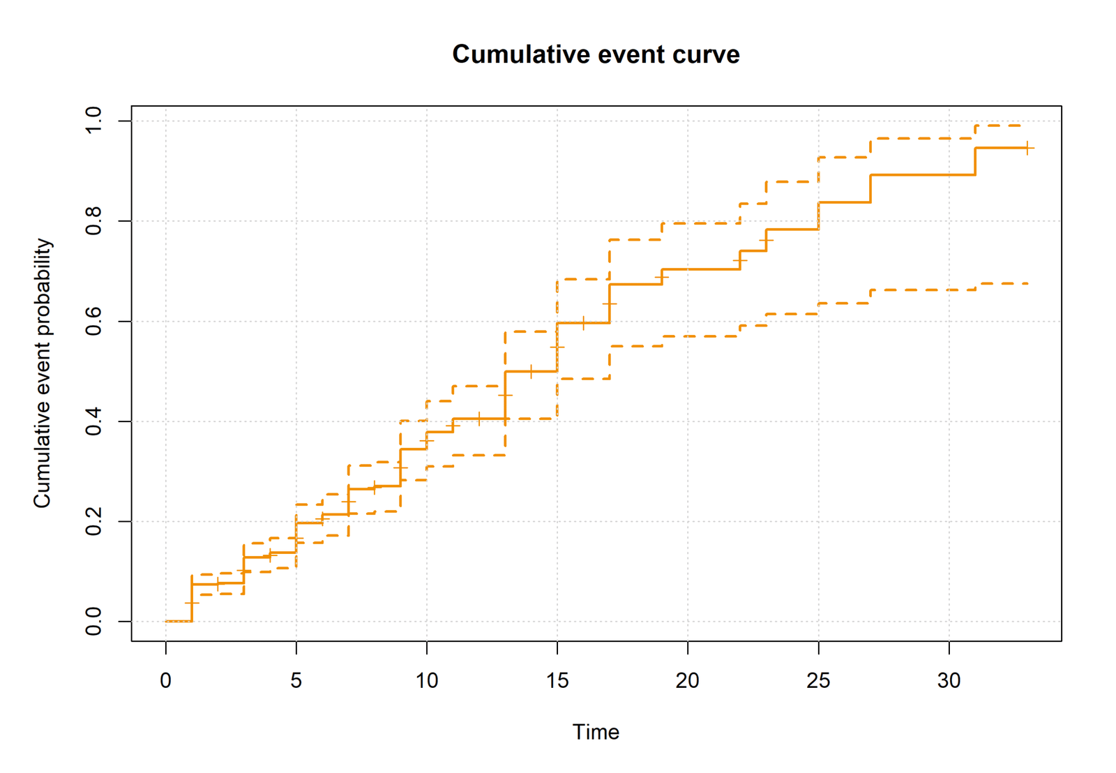
The unadjusted constructed Kaplan-Meier survival is 0.926040 at time 1, 0.872042 at time 3, 0.803402 at time 5, 0.500356 at time 13 and 0.054133 at time 31. Tail values have less support because few records remain at risk.
Tied Events
Breslow reuses the full risk-set denominator across the tied event set. Efron removes fractional tied-event contributions sequentially. With heavily tied integer times, the selected approximation can materially affect coefficients and standard errors.
Variables Used, Coding and Standardization
The outcome construction and predictor roles must remain fixed across software. The nine-term Python and R models deliberately exclude variables used to create time or event status.
| Field | Role | Rule or contrast | Interpretive consequence |
|---|---|---|---|
| cox_time | Constructed duration | absences + 1; range 1 to 33 | One unit is an absence-count step, not prospective follow-up time. |
| cox_event | Constructed event | G3 < 10 or failures > 0 | 151 events; composite educational teaching endpoint. |
| Censored status | Constructed complement | Neither event condition met | 498 records; not natural loss-to-follow-up censoring. |
| G1, G2 | Numeric predictors | One grade-point contrast | Earlier and more recent prior achievement. |
| studytime | Numeric coded predictor | One study-time category | Assumed linear on the log-hazard scale. |
| age | Numeric predictor | One year | Assumed linear on the log-hazard scale. |
| Medu, Fedu | Numeric coded predictors | One education-code step | Equal spacing is assumed unless indicators or splines are used. |
| school | Indicator | MS versus GP | GP is the nine-term reference. |
| sex | Indicator | Male versus female | Female is the nine-term reference. |
| address | Indicator | Urban versus rural | Rural is the nine-term reference. |
| G3, failures | Event construction | Excluded from predictors | Prevents direct reuse of endpoint-defining information. |
| absences | Time construction | Excluded from predictors | Prevents direct reuse of the constructed time variable. |
Verified Cox Regression Results
Model and Software Summary
| Evidence source | Cases / events | Predictors | Tie method stated | Global or fit evidence | Primary use |
|---|---|---|---|---|---|
| Python PHReg | 649 / 151 | 9 | Breslow | Log partial likelihood −707.145324; partial AIC 1432.290648 | Corrected nine-term coefficient and risk-score analysis. |
| R coxph | 649 / 151 | 9 | Efron | LR χ²(9) = 236.168740, p = 8.2526 × 10−46; concordance 0.857725 | Nine-term cross-check and formal PH tests. |
| SPSS primary COXREG | 649 / 151 | 13 | Not stated in saved syntax | Change χ²(13) = 215.671, p < .001; −2LL = 1405.051 | Broader specification sensitivity rather than direct replication. |
Nine-Term Python and R Hazard Ratios
| Term | Python HR | Python p | R HR | R p | Combined reading |
|---|---|---|---|---|---|
| G1 | 0.822437 | 0.000258 | 0.833922 | 0.000910 | Higher prior grade is associated with lower constructed event hazard. |
| G2 | 0.820490 | 3.043 × 10⁻⁷ | 0.776380 | 3.898 × 10⁻¹⁰ | Strongest grade evidence; tie methods alter the exact magnitude. |
| studytime | 0.947487 | 0.676690 | 0.929514 | 0.576997 | Intervals cross one in both models. |
| age | 1.022861 | 0.724809 | 1.031350 | 0.632455 | No clear linear age effect. |
| Medu | 0.940283 | 0.530111 | 0.947155 | 0.580252 | No clear linear maternal-education effect. |
| Fedu | 0.936678 | 0.533836 | 0.936901 | 0.532764 | Nearly identical inconclusive estimates. |
| MS school vs GP | 1.985538 | 0.001644 | 2.123581 | 0.000606 | Approximately doubled fitted hazard, with wide uncertainty. |
| Male vs female | 1.102033 | 0.579820 | 1.108593 | 0.560159 | Intervals cross one. |
| Urban vs rural | 0.705148 | 0.048444 | 0.665191 | 0.021239 | Lower hazard in nine-term models; estimate is specification sensitive. |
Broader SPSS Primary Model
| SPSS term | Hazard ratio | p-value | 95% CI | Interpretation |
|---|---|---|---|---|
| G1 | 0.814 | < .001 | 0.732 to 0.905 | Protective grade association remains. |
| G2 | 0.823 | < .001 | 0.763 to 0.888 | Protective grade association remains. |
| studytime | 0.944 | 0.655 | 0.734 to 1.214 | Inconclusive. |
| age | 1.020 | 0.785 | 0.885 to 1.175 | Inconclusive. |
| Medu | 0.985 | 0.886 | 0.805 to 1.205 | Inconclusive. |
| Fedu | 0.926 | 0.465 | 0.752 to 1.139 | Inconclusive. |
| traveltime | 1.075 | 0.525 | 0.860 to 1.344 | Added SPSS covariate; inconclusive. |
| health | 1.189 | 0.004 | 1.056 to 1.338 | Higher coded health is associated with higher constructed hazard. |
| MS school vs GP | 2.130 | 0.001 | 1.379 to 3.291 | Large positive school contrast persists. |
| Male vs female | 1.017 | 0.923 | 0.716 to 1.445 | Inconclusive. |
| Urban vs rural | 0.781 | 0.187 | 0.541 to 1.128 | No longer below .05 after broader adjustment. |
| Higher intention | 0.897 | 0.605 | 0.595 to 1.353 | Inconclusive. |
| Internet access | 0.873 | 0.495 | 0.591 to 1.290 | Inconclusive. |
Python Charts and Diagnostic Explanations
The first five stories use Python-side or Python-companion visuals. The sixth displays the formal R Schoenfeld-test probabilities in the same chart-story layout so the diagnostic conclusion is not separated from the visual evidence.
Chart 1: Constructed Survival-Time Distribution
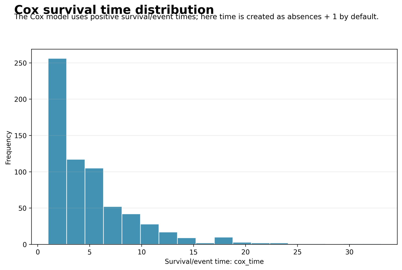
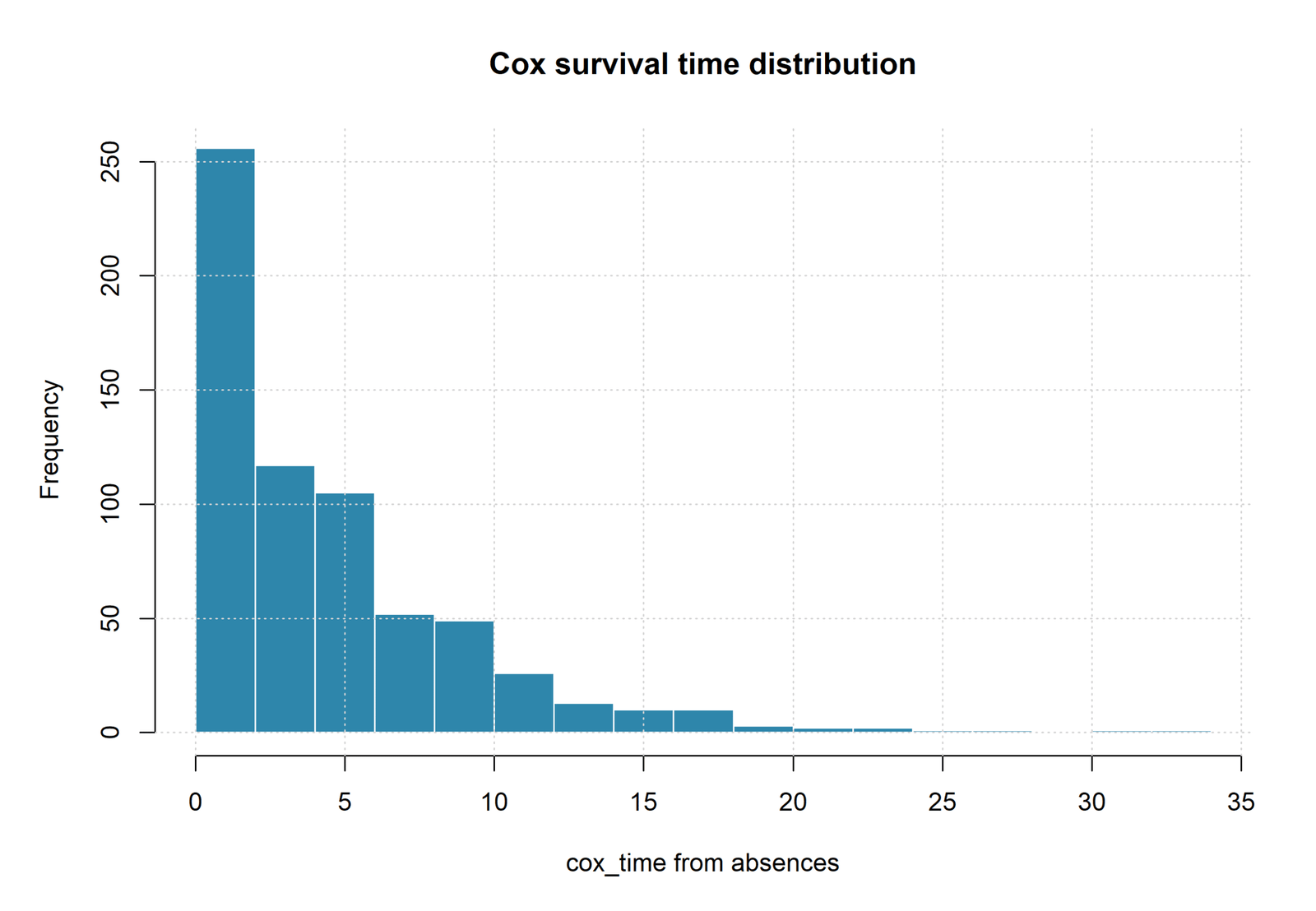
The distribution is strongly right skewed and concentrated at low integer values.
Mean = 4.659476, median = 3, first quartile = 1 and third quartile = 7.
The discrete scale creates many tied event and censoring times, making the tie approximation important.
The chart also shows why the scale should not be described as ordinary prospective follow-up.
Chart 2: Event and Censoring Counts
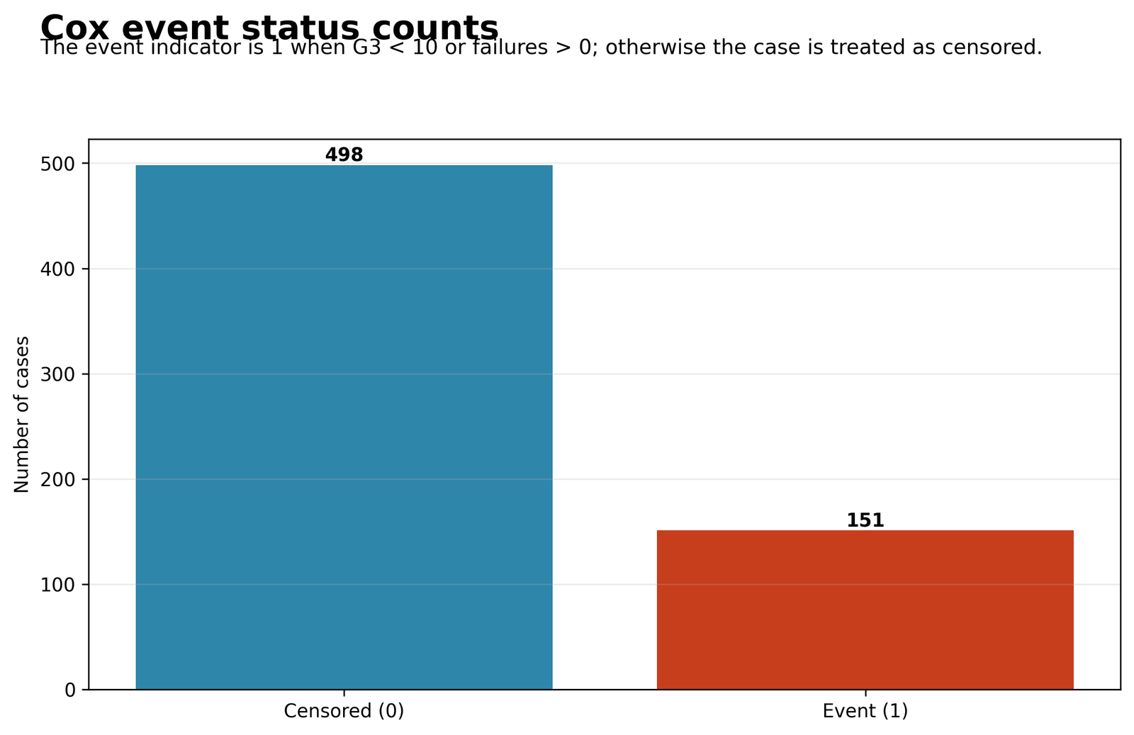
Censored labels substantially outnumber observed constructed events.
151 events and 498 censored records; event fraction = 0.232666.
Events arise from the union of 100 low-G3 records and 100 prior-failure records with 49 overlapping.
The event count supports nine slopes more comfortably than the broader 13-term SPSS model.
Chart 3: Overall Kaplan-Meier Curve
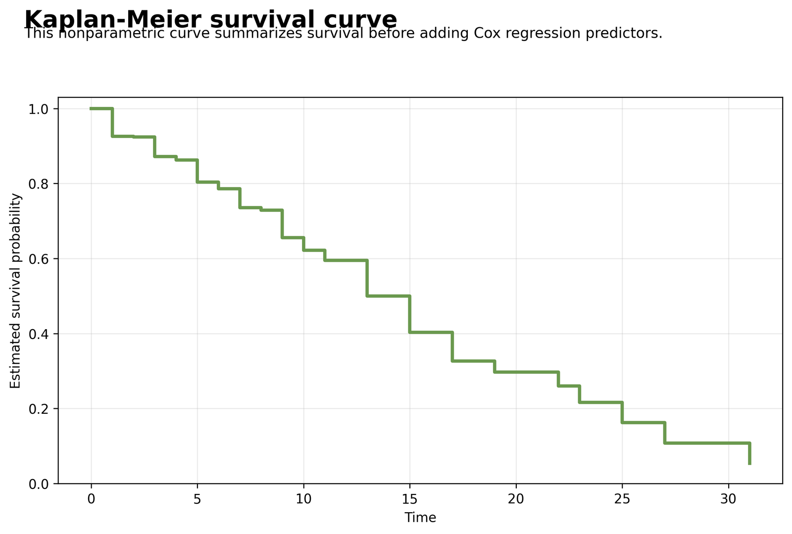
The curve drops at event times and becomes increasingly uncertain in the sparse tail.
S(1) = 0.926040, S(5) = 0.803402, S(13) = 0.500356 and S(31) = 0.054133.
Censoring reduces later risk sets but does not directly create downward survival steps.
The nonparametric curve verifies the time-event construction before multivariable modeling.
Chart 4: Python Baseline Survival for the Raw-Zero Profile
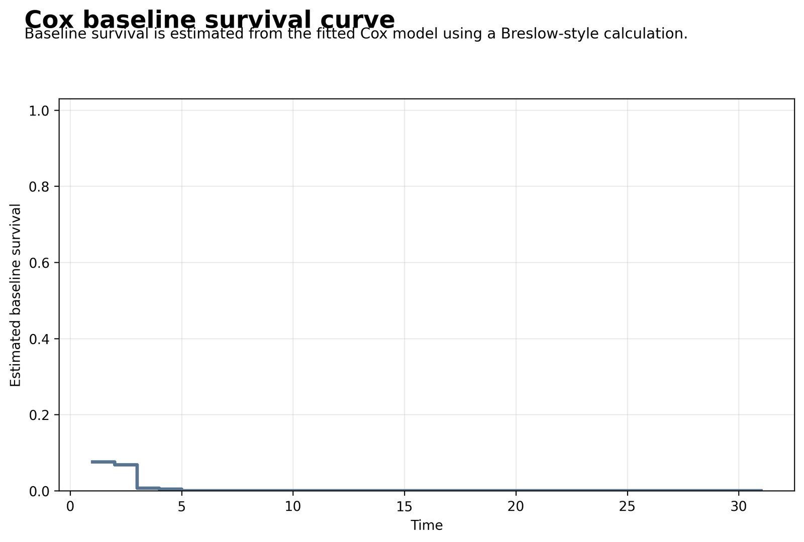
The baseline curve falls extremely quickly.
Baseline survival is 0.075484 at time 1 and 0.006478 at time 3.
The reference includes age zero and grade zero, so the steep curve is mathematically consistent but substantively unrealistic.
Absolute survival curves must identify the covariate profile and centering convention.
Chart 5: Log-Minus-Log Proportional-Hazards Visual
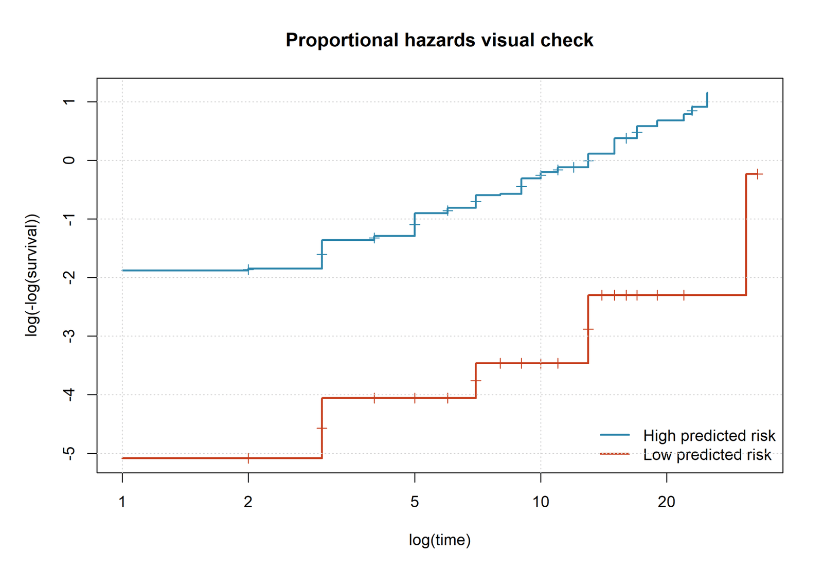
The transformed high- and low-risk curves are separated but not perfectly parallel.
Python forms 325 high-risk and 324 low-risk records.
The groups are derived from the complete score, so the graph is not a term-specific PH test.
The visual motivates formal Schoenfeld residual testing rather than replacing it.
Chart 6: Formal Proportional-Hazards Test Probabilities
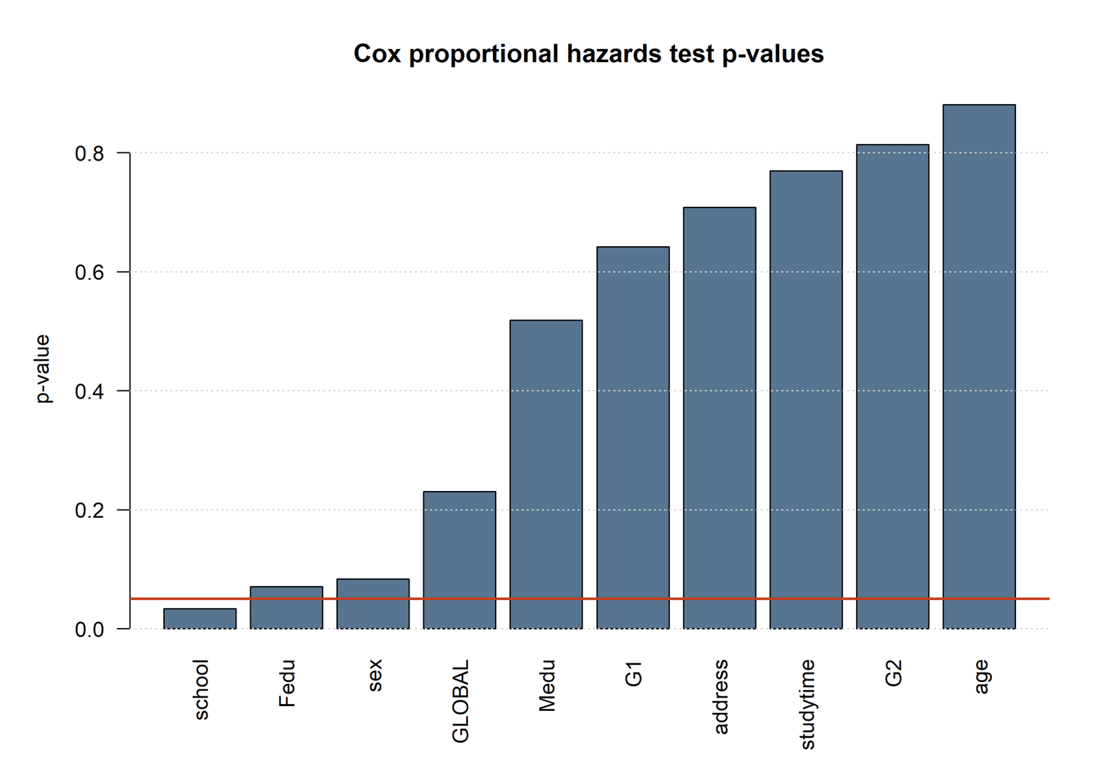
School is the only term below 0.05; the global test remains above the threshold.
School p = 0.033876, Fedu p = 0.070962, sex p = 0.083323 and global p = 0.230437.
The overall model does not show broad PH failure, but a term-specific school signal remains.
A global nonrejection should not be used to dismiss a predictor-level diagnostic concern.
R Charts and Paired Explanations
The R visuals use Efron ties and the same nine-term predictor set. They are arranged in two paired rows with one explanation box behind each chart.
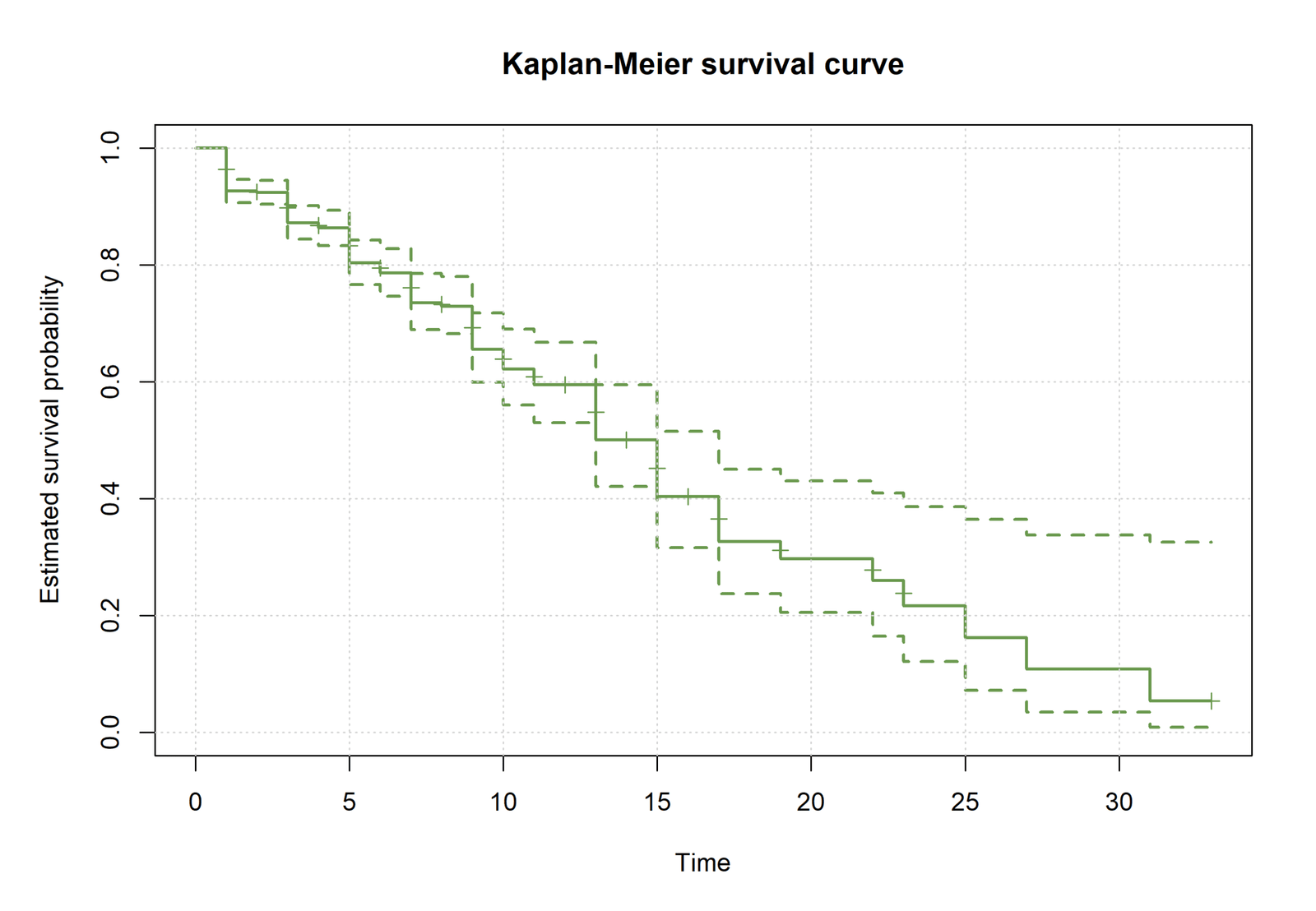
R Chart 1: Kaplan-Meier Survival
Pattern: Survival falls in steps and the tail becomes thin after earlier events and censoring.
Key values: The verified overall curve is 0.926040 at time 1 and approximately 0.500356 at time 13.
Interpretation: The curve describes the constructed outcome before covariate adjustment.
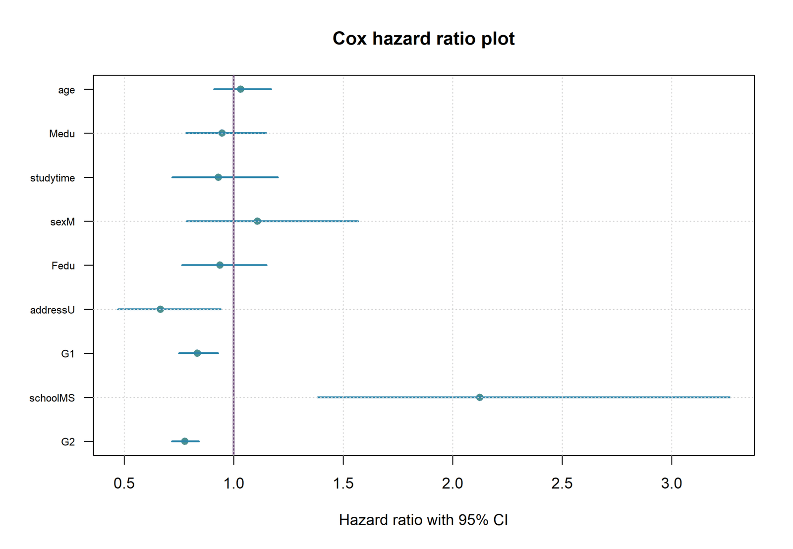
R Chart 2: Hazard-Ratio Forest Plot
Pattern: G1, G2 and address lie below one, while MS school lies above one. Five intervals cross one.
Key values: G2 HR = 0.776380; school HR = 2.123581; address HR = 0.665191.
Interpretation: The logarithmic scale presents reciprocal departures from one symmetrically.
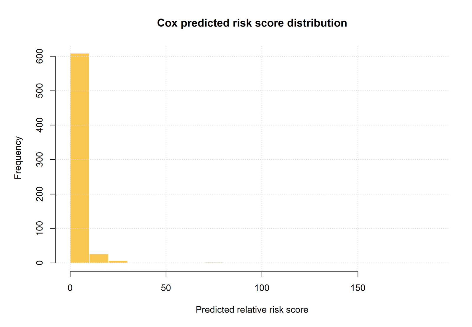
R Chart 3: Relative-Risk Distribution
Pattern: Scores are highly right skewed, with a small number of very large values.
Key values: Range = 0.033921 to 186.597630, median = 0.917373 and mean = 3.521240.
Interpretation: Absolute score scale depends on centering; ranking is the more portable quantity.
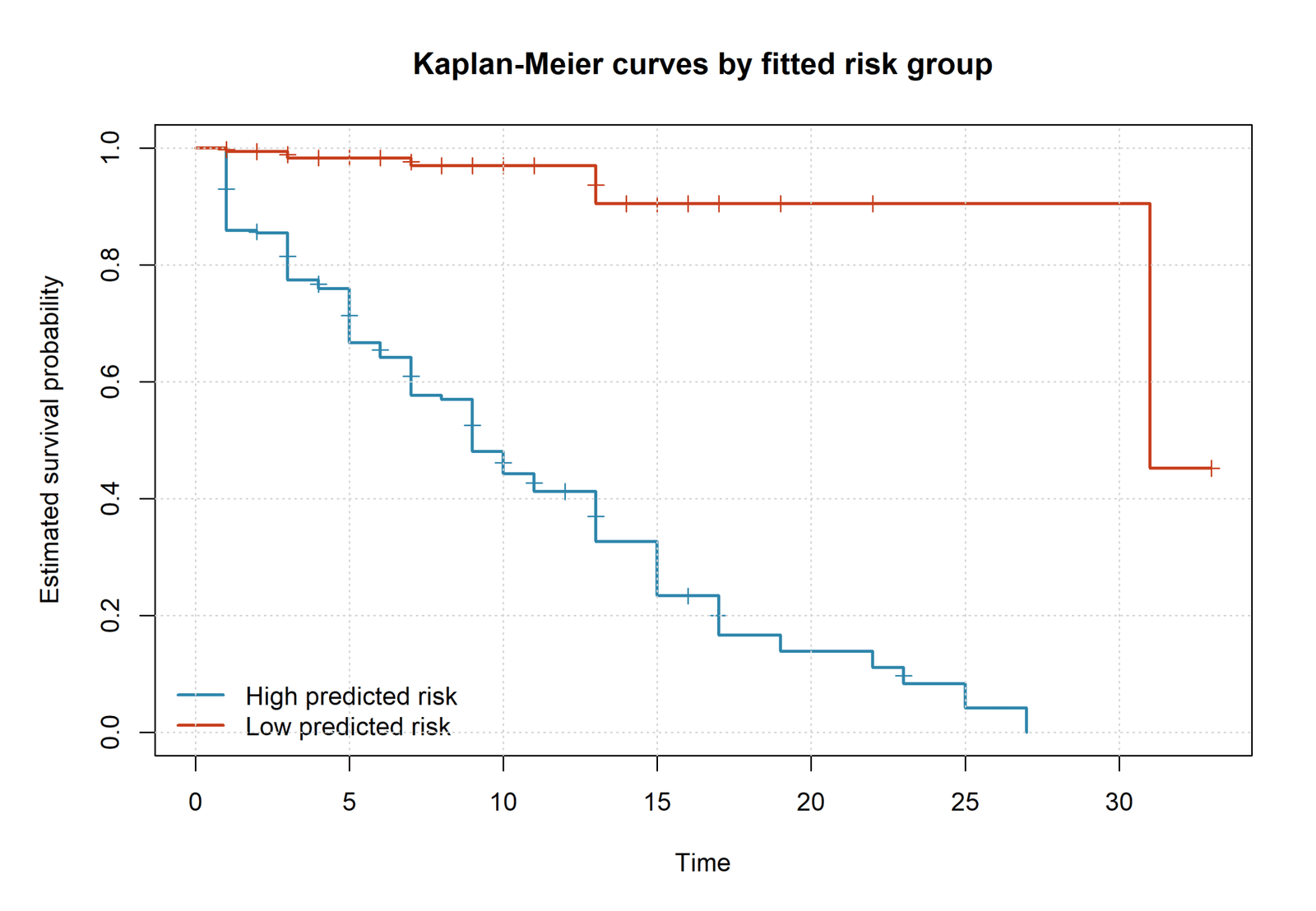
R Chart 4: Kaplan-Meier Curves by Risk Group
Pattern: High- and low-score groups separate sharply.
Key values: The high-score half contains 144 of 151 events; the low-score half contains 7.
Interpretation: The model strongly ranks the same data used for fitting, especially through prior grades.
Cox Regression Coefficient and Parameter Interpretation
G1 and G2
Python estimates G1 B = −0.195483 and HR = 0.822437. Holding the other eight terms fixed, one additional G1 point is associated with a 17.756% lower fitted hazard. G2 B = −0.197854 and HR = 0.820490, corresponding to a 17.951% lower fitted hazard per point.
R estimates similar directions but different magnitudes under Efron ties: G1 HR = 0.833922 and G2 HR = 0.776380. The two prior grades are entered simultaneously, so each slope represents information beyond the other grade.
School
Python estimates MS versus GP HR = 1.985538, 95% CI [1.295446, 3.043246]. R estimates HR = 2.123581, 95% CI [1.380789, 3.265956]. The point estimates are large, but the intervals are broad and the R school PH test is 0.033876.
Address
Urban versus rural has Python HR = 0.705148 and R HR = 0.665191 in the nine-term models. The Python upper interval limit is 0.997614, so the result is close to the no-effect boundary. In the broader SPSS model, HR = 0.781 and p = 0.187.
Inconclusive Terms
studytime, age, Medu, Fedu and sex have nine-term intervals crossing one. This does not prove exact equivalence. It indicates limited evidence against HR = 1 under the specified linear forms and constructed endpoint.
Predictions, Effects and Model Meaning
Cox Regression prediction has two layers. The linear predictor xβ or relative-risk score exp(xβ) ranks profiles. Absolute survival at time t additionally requires the baseline survival S₀(t).
Python stores uncentered risk scores with median 0.009880, mean 0.028624 and range 0.000512 to 1.039230. R stores scores under a different centering convention with median 0.917373, mean 3.521240 and range 0.033921 to 186.597630. Their raw scales are not comparable, but their within-software rankings are meaningful.
The supplied Python median split contains 325 high-risk and 324 low-risk records. High-group survival is 0.858462 at time 1, 0.665391 at time 5 and 0.325878 at time 13. Low-group survival is much higher at the same early points.
The raw-zero Python baseline survival is not an average-student prediction. It evaluates zero for G1, G2, studytime, age, Medu and Fedu along with the categorical references. A realistic profile should use meaningful values and a consistently reconstructed baseline.
Cox Regression Assumptions and Diagnostics
Global R p = 0.230437; school p = 0.033876 requires follow-up.
The constructed absence-based time is not a genuine follow-up duration.
Python/R use nine terms; the SPSS primary model uses thirteen.
Proportional-Hazards Evidence
Term p-values are G1 0.641900, G2 0.813277, studytime 0.769363, age 0.880921, Medu 0.518286, Fedu 0.070962, school 0.033876, sex 0.083323 and address 0.708263. The global p-value is 0.230437.
Functional Form
No saved spline or nonlinear comparison is available. Treating studytime, Medu and Fedu as equally spaced numeric scores and age and grades as linear log-hazard terms remains an assumption.
Independent Observations
Each row represents one student, but students can share school and social context. Ordinary standard errors do not model residual clustering beyond the included school indicator.
Censoring
Noninformative censoring is not naturally assessable because censoring is created by the outcome rule rather than an observation process. This is the most important limitation of the example.
Influence and Stability
Risk scores are highly skewed and school has a large hazard ratio. DFBETA, deviance residuals, score residuals and leave-one-cluster or bootstrap stability checks would strengthen a substantive analysis.
Cox Regression in Python, R, SPSS and Excel
Python
statsmodels PHReg fits the corrected nine-term model with explicitly requested Breslow ties.
- 649 cases and 151 events
- Log partial likelihood −707.145324
- Partial AIC 1432.290648
- Risk-score ledger for all 649 rows
R
survival::coxph fits the same right-hand side with Efron ties and formal cox.zph diagnostics.
- LR χ²(9) = 236.168740
- Concordance = 0.857725
- Global PH p = 0.230437
- School PH p = 0.033876
SPSS
The primary COXREG output adds traveltime, health, higher intention and internet access.
- 13 predictors
- Model change χ² = 215.671
- Health and school below .05
- Address p = 0.187
Excel
The corrected workbook audits time/event construction, hazard-ratio transformations and Kaplan-Meier arithmetic.
- Eight-row worked setup
- Coefficient-to-HR formulas
- Synthetic Kaplan-Meier sheet
- Not a full 649-row partial-likelihood engine
Code: Expand Only the Software You Need
Python Cox Regression with Breslow ties
from pathlib import Path
import numpy as np
import pandas as pd
from statsmodels.duration.hazard_regression import PHReg

DATA = Path("dataset.csv")
NUMERIC = ["G1", "G2", "studytime", "age", "Medu", "Fedu"]
CATEGORICAL = ["school", "sex", "address"]

df = pd.read_csv(DATA)
required = ["absences", "G3", "failures"] + NUMERIC + CATEGORICAL
dat = df[required].dropna().copy()

# Teaching construction used by the supplied files.
dat["cox_time"] = dat["absences"].abs() + 1
dat["cox_event"] = (
    (dat["G3"] < 10) | (dat["failures"] > 0)
).astype(int)

X = pd.get_dummies(
    dat[NUMERIC + CATEGORICAL],
    columns=CATEGORICAL,
    drop_first=True,
    dtype=float,
)

fit = PHReg(
    endog=dat["cox_time"].astype(float),
    exog=X.astype(float),
    status=dat["cox_event"].astype(int),
    ties="breslow",
).fit(disp=False)

ci = np.asarray(fit.conf_int())
coef = pd.DataFrame({
    "term": X.columns,
    "log_hazard_B": fit.params,
    "standard_error": fit.bse,
    "z": fit.params / fit.bse,
    "p_value": fit.pvalues,
    "hazard_ratio": np.exp(fit.params),
    "hr_lower": np.exp(ci[:, 0]),
    "hr_upper": np.exp(ci[:, 1]),
})

linear_predictor = X.to_numpy() @ fit.params
relative_risk = np.exp(linear_predictor)
median_risk = float(np.median(relative_risk))

risk_audit = pd.DataFrame({
    "row": np.arange(1, len(dat) + 1),
    "constructed_time": dat["cox_time"].to_numpy(),
    "event": dat["cox_event"].to_numpy(),
    "linear_predictor": linear_predictor,
    "relative_risk": relative_risk,
    "risk_group": np.where(
        relative_risk >= median_risk,
        "High predicted risk",
        "Low predicted risk",
    ),
})

summary = pd.DataFrame([{
    "n": len(dat),
    "events": int(dat["cox_event"].sum()),
    "censored": int((1 - dat["cox_event"]).sum()),
    "tie_method": "Breslow",
    "log_partial_likelihood": float(fit.llf),
    "partial_aic_9_parameters": float(2 * 9 - 2 * fit.llf),
}])

coef.to_csv("cox_python_coefficients.csv", index=False)
risk_audit.to_csv("cox_python_risk_audit.csv", index=False)
summary.to_csv("cox_python_summary.csv", index=False)
print(fit.summary())
R Cox Regression with Efron ties and cox.zph
library(survival)

raw <- read.csv("dataset.csv", stringsAsFactors = FALSE)
vars <- c(
  "absences", "G3", "failures", "G1", "G2", "studytime",
  "age", "Medu", "Fedu", "school", "sex", "address"
)
d <- na.omit(raw[vars])

d$cox_time <- abs(d$absences) + 1
d$cox_event <- as.integer(d$G3 < 10 | d$failures > 0)
d$school <- relevel(factor(d$school), ref = "GP")
d$sex <- relevel(factor(d$sex), ref = "F")
d$address <- relevel(factor(d$address), ref = "R")

fit <- coxph(
  Surv(cox_time, cox_event) ~
    G1 + G2 + studytime + age + Medu + Fedu +
    school + sex + address,
  data = d,
  ties = "efron",
  model = TRUE,
  x = TRUE
)

s <- summary(fit)
ph <- cox.zph(fit)
base_km <- survfit(Surv(cox_time, cox_event) ~ 1, data = d)
risk <- predict(fit, type = "risk")
risk_group <- ifelse(risk >= median(risk), "High", "Low")
group_km <- survfit(
  Surv(cox_time, cox_event) ~ risk_group,
  data = d
)

coef_table <- data.frame(
  term = rownames(s$coefficients),
  log_hazard_B = s$coefficients[, "coef"],
  standard_error = s$coefficients[, "se(coef)"],
  z = s$coefficients[, "z"],
  p_value = s$coefficients[, "Pr(>|z|)"],
  hazard_ratio = s$conf.int[, "exp(coef)"],
  hr_lower = s$conf.int[, "lower .95"],
  hr_upper = s$conf.int[, "upper .95"],
  row.names = NULL
)

write.csv(coef_table, "cox_r_coefficients.csv", row.names = FALSE)
write.csv(as.data.frame(ph$table), "cox_r_ph_tests.csv")
write.csv(
  data.frame(
    row = seq_len(nrow(d)),
    constructed_time = d$cox_time,
    event = d$cox_event,
    relative_risk = risk,
    risk_group = risk_group
  ),
  "cox_r_risk_audit.csv",
  row.names = FALSE
)

print(s)
print(ph)
SPSS primary and nine-term comparison syntax
* Teaching time and event variables used in the supplied package.
COMPUTE cox_time = ABS(absences) + 1.
COMPUTE cox_event = (G3 < 10 OR failures > 0).
EXECUTE.

* Primary SPSS model in the supplied PDF uses 13 predictors.
COXREG cox_time
 /STATUS=cox_event(1)
 /METHOD=ENTER
   G1 G2 studytime age Medu Fedu traveltime health
   school_MS sex_M address_U higher_yes internet_yes
 /CONTRAST (school_MS)=Indicator
 /CONTRAST (sex_M)=Indicator
 /CONTRAST (address_U)=Indicator
 /CONTRAST (higher_yes)=Indicator
 /CONTRAST (internet_yes)=Indicator
 /PRINT=CI(95).

* Nine-term comparison matching the Python/R right-hand side.
COXREG cox_time
 /STATUS=cox_event(1)
 /METHOD=ENTER
   G1 G2 studytime age Medu Fedu school_MS sex_M address_U
 /PRINT=CI(95).

* The saved primary command does not state a tie option.
* Do not label the SPSS coefficients Breslow or Efron unless the
* installed procedure/output explicitly verifies that setting.
Excel construction, hazard-ratio and Kaplan-Meier formulas
Excel formulas and manual checks

1. Constructed time
=ABS([@absences])+1

2. Event indicator
=IF(OR([@G3]<10,[@failures]>0),1,0)

3. Hazard ratio from a fitted log-hazard coefficient
=EXP([@coefficient])

4. Lower 95% hazard-ratio limit
=EXP([@coefficient]-1.96*[@standard_error])

5. Upper 95% hazard-ratio limit
=EXP([@coefficient]+1.96*[@standard_error])

6. Linear predictor for one profile
=SUMPRODUCT(PredictorValueRange,CoefficientRange)

7. Relative-risk score
=EXP(LinearPredictorCell)

8. One Kaplan-Meier step
=PreviousSurvival*(1-EventsAtTime/AtRiskBeforeTime)

Important:
- Excel can audit coding, hazard ratios and Kaplan-Meier arithmetic.
- The corrected workbook contains a small worked setup, not a full
  replacement for partial-likelihood optimization on all 649 rows.
- A survival probability requires a baseline survival estimate at a
  specified time; EXP(linear predictor) alone is not a probability.
Advanced Cox Regression Topics
These 26 panels extend the worked Cox Regression analysis from risk-set mechanics and tied events through proportionality, baseline survival, validation and responsible reporting.
1. Cox Regression Estimand
Cox Regression estimates conditional hazard ratios for a time-to-event process. A coefficient compares instantaneous event rates among records that are still in the risk set, while leaving the baseline hazard unspecified.
In this package, the estimand is tied to a constructed absence-based time and a composite academic event. The mechanics are valid for teaching, but the estimand is not a literal prospective failure hazard.
2. Genuine Time Origin and Endpoint
A substantive Cox Regression study requires a clearly defined start time, event time, censoring time and endpoint. Every subject must enter the risk set under a common or explicitly modeled time origin.
The current time variable is absences plus one and does not represent elapsed follow-up. A real study should replace it with recorded duration from an educationally meaningful origin.
3. Composite Event Construction
The supplied event equals one when G3 is below 10 or failures exceeds zero. Exactly 100 records meet each condition and 49 meet both, producing 151 unique events.
Composite endpoints should combine components with compatible clinical or substantive meaning. Here, a final-grade criterion and prior-failure history are joined for demonstration rather than because a prospective endpoint was observed.
4. Censoring Interpretation
Censoring normally means the event time is unknown beyond the observed follow-up. It is not the same as declaring that an event never occurred.
The 498 censored labels in this package are assigned by the complement of the constructed event rule, not by loss to follow-up or study closure. Noninformative-censoring assumptions therefore cannot be assessed in their usual form.
5. Partial Likelihood
Cox Regression estimates slopes by comparing the covariates of each event record with all records still at risk at that event time. The baseline hazard cancels from these risk-set ratios.
Partial likelihood uses event ordering and risk-set membership rather than a fully specified survival-time density. This is why tie handling matters when many records share integer-valued constructed times.
6. Breslow Tie Handling
The corrected Python PHReg analysis explicitly uses Breslow handling. At a tied time, Breslow reuses the full risk-set denominator for each event in the tied set.
Breslow is computationally convenient but can differ from Efron when ties are numerous. Its coefficients should be reported as the Python result rather than pooled with R decimals.
7. Efron Tie Handling
The R coxph analysis explicitly uses Efron handling. Efron gradually removes fractions of the tied-event contribution across the tied set and often approximates the exact discrete likelihood more closely.
R estimates G2 HR = 0.776380, whereas Python estimates 0.820490. The difference is expected when tie approximations and software implementations differ.
8. Exact and Discrete-Time Alternatives
An exact tied-event method can be considered when event times are genuinely discrete and tied sets are manageable. A discrete-time hazard model is another option when time is observed in intervals.
The present absence-count scale creates heavy ties by construction. A real application should decide whether continuous-time Cox Regression or a discrete-time model better matches data collection.
9. Proportional Hazards
Proportional hazards requires a covariate hazard ratio to remain constant over the modeled time scale. The baseline hazard may vary, but the multiplicative contrast is time invariant unless a time-varying effect is specified.
The R global Schoenfeld test has p = 0.230437, while school has p = 0.033876. The global result is reassuring only model-wide; the school term still deserves targeted follow-up.
10. Schoenfeld Residual Tests
Scaled Schoenfeld residual tests evaluate whether coefficient residual patterns are associated with transformed event time. A small term-specific p-value indicates evidence against a constant coefficient.
G1, G2, studytime, age, Medu and address show no supplied term-specific signal. Fedu and sex sit above 0.05 but are close enough to justify graphical review.
11. Log-Minus-Log Curves
Approximately parallel log-minus-log survival curves can support proportionality for a categorical grouping. Crossing or strongly nonparallel curves can indicate time-varying effects.
The supplied grouping is created from the fitted multivariable score, so it is only a coarse visual check. It cannot replace term-level Schoenfeld residual diagnostics.
12. Time-Varying Effects
When proportionality fails, a predictor can be interacted with a function of time or modeled through a stratified or extended Cox Regression specification.
A time-varying school effect is one possible follow-up because the school PH test is below 0.05. The form should be prespecified or validated rather than chosen solely to remove a diagnostic p-value.
13. Stratification
Stratified Cox Regression allows separate baseline hazards across strata while estimating common slopes for the remaining predictors. The stratifying variable does not receive a single hazard ratio.
Stratifying by school could address a school-specific baseline pattern, but it would change the scientific question and remove the direct school hazard-ratio estimate.
14. Functional Form of Numeric Predictors
Cox Regression assumes each numeric term is linear on the log-hazard scale unless another basis is specified. Grade points, age and coded education steps may not satisfy that assumption.
Restricted cubic splines or indicator coding can test nonlinear forms. Any added flexibility consumes event information and must be evaluated without reusing outcome-construction variables as predictors.
15. Reference Categories
The nine-term Python and R models use GP school, female sex and rural address as reference categories. Indicator hazard ratios compare MS with GP, male with female and urban with rural.
Changing a reference category changes coefficient signs and labels but not fitted risk ordering. Cross-software comparisons require identical dummy coding.
16. Hazard Ratio versus Probability
A hazard ratio compares instantaneous event rates, not cumulative probabilities. HR = 0.820490 corresponds to a 17.951 percent lower fitted hazard per G2 point, conditional on the model.
It does not imply a 17.951 percent lower event probability at every time. Survival probabilities require the baseline survival function and a specified covariate profile.
17. Multi-Unit Contrasts
For a multi-unit numeric contrast, exponentiate the coefficient multiplied by the contrast. A five-point G2 contrast is exp(5B), not five times the one-point hazard ratio.
Reporting meaningful contrasts can improve interpretation when one-unit changes are too small or coded categories are not naturally unit spaced.
18. Baseline Survival and Centering
Baseline survival is defined for the covariate reference used by the software. Python reconstructs a raw all-zero profile that includes age zero and grade zero, which is mathematically valid but substantively unrealistic.
R may center covariates when reporting baseline quantities. Absolute baseline curves therefore cannot be compared without reconstructing the same profile and centering convention.
19. Relative-Risk Scores
The relative-risk score exp(xβ) ranks profiles by fitted hazard. Its absolute numerical scale depends on coefficient centering and the covariate reference.
Python scores have median 0.009880 and mean 0.028624, whereas R scores have median 0.917373 and mean 3.521240. Ranking is comparable; the raw scales are not.
20. Concordance
Concordance measures whether higher fitted risk tends to correspond to earlier events among usable pairs. R reports 0.857725 for the constructed endpoint.
Concordance is a discrimination measure, not R-squared and not calibration. It should not be translated into the percentage of outcomes explained.
21. Calibration
A Cox Regression model can rank risk well while producing inaccurate absolute survival probabilities. Calibration requires comparing predicted and observed survival at prespecified times or across risk groups.
The supplied package emphasizes ranking and Kaplan-Meier separation but does not provide an independent calibration assessment for a genuine prospective endpoint.
22. Events per Parameter
The nine-term models use 151 events for nine coefficients, while the primary SPSS model uses 13 coefficients. Event information must support the number of terms, nonlinearities and interactions.
The raw ratio is more comfortable for nine terms than 13, but it does not guarantee stable estimates. Bootstrap or repeated-sample validation is still valuable.
23. Clustering and Dependence
Ordinary Cox Regression assumes independent subject-level contributions. Students may share school, classroom, neighborhood or social contexts that create correlated outcomes.
Robust sandwich covariance or frailty and multilevel survival methods may be needed when the sampling design contains clusters beyond the included school indicator.
24. SPSS Specification Difference
The SPSS primary model adds traveltime, health, higher-education intention and internet access to the nine-term right-hand side. Its address estimate therefore answers a different adjusted question.
Address has p = 0.187 in the broader SPSS run but remains below 0.05 in Python and R. This is specification sensitivity, not proof that one software calculation is wrong.
25. Validation and Optimism
The same 649 records define the outcome, estimate coefficients, form risk groups and display discrimination. Apparent separation is therefore descriptive and can be optimistic.
Bootstrap validation or an external cohort should evaluate concordance, calibration and coefficient stability after every modeling decision is fixed.
26. Cox Regression Decision Framework
Use Cox Regression only after verifying a genuine time origin, event definition, censoring process and risk-set interpretation. Declare tie handling, predictor coding, functional forms and proportional-hazards checks.
Report coefficients with hazard-ratio intervals, keep software specifications separate and validate discrimination and calibration. In the present package, treat the analysis as a detailed teaching demonstration rather than a real causal or prospective survival study.
- Cox Regression requires a genuine time origin and event process.
- Cox Regression estimates hazard ratios rather than direct probability differences.
- Cox Regression should state the tied-event method.
- Cox Regression should report proportional-hazards diagnostics.
- Cox Regression should separate software specifications.
- Cox Regression should validate discrimination and calibration.
- Cox Regression begins with a defensible time origin.
- Cox Regression requires a prespecified event definition.
- Cox Regression distinguishes censoring from permanent event absence.
- Cox Regression estimates conditional hazard ratios.
- Cox Regression does not convert a hazard ratio directly into probability change.
- Cox Regression uses risk sets at observed event times.
- Cox Regression should disclose the tied-event approximation.
- Cox Regression should report categorical reference groups.
- Cox Regression should evaluate numeric functional form.
- Cox Regression should report proportional-hazards evidence.
- Cox Regression should distinguish global and term-specific diagnostics.
- Cox Regression should identify the baseline-survival reference profile.
- Cox Regression should report concordance as discrimination, not explained variation.
- Cox Regression should examine calibration before absolute-risk use.
- Cox Regression should keep different software specifications separate.
- Cox Regression should preserve the risk-score audit trail.
- Cox Regression should validate optimism from in-sample risk groups.
- Cox Regression should avoid causal claims from observational coefficients.
- Cox Regression should use genuine longitudinal data for substantive survival claims.
- Cox Regression should report limitations beside the numerical results.
APA-Style Reporting
Using 649 complete student records, time was operationalized as absences plus one and the event as G3 below 10 or any prior failure, yielding 151 events and 498 censored labels. An Efron-tied Cox Regression model included G1, G2, studytime, age, maternal education, paternal education, school, sex and address. The model improved on the null partial likelihood, likelihood-ratio χ²(9) = 236.17, p < .001, and concordance was .858.
Higher G1 was associated with a lower fitted event hazard, HR = 0.834, 95% CI [0.749, 0.928], p = .001, as was higher G2, HR = 0.776, 95% CI [0.717, 0.840], p < .001. MS school was associated with a higher fitted hazard than GP, HR = 2.124, 95% CI [1.381, 3.266], p = .001, and urban address with a lower fitted hazard than rural address, HR = 0.665, 95% CI [0.470, 0.941], p = .021.
The global Schoenfeld-residual test did not reject proportional hazards, p = .230, although the school term had p = .034 and required follow-up. The report must state that the duration, event and censoring indicators were constructed for teaching and do not represent a genuine prospective survival process.
Publication Checklist
- State the exact time origin and duration unit.
- State the exact event and censoring rules.
- Report 649 records, 151 events and 498 censored labels.
- Disclose that the survival outcome is constructed.
- List the nine Python/R predictors.
- State GP, female and rural references.
- State Breslow ties for Python.
- State Efron ties for R.
- Keep the 13-term SPSS model separate.
- Report hazard ratios with confidence intervals.
- Do not translate hazard ratios into direct probability changes.
- Report concordance as discrimination, not R².
- Report global and term-specific PH tests.
- Explain the school PH concern.
- Identify the raw-zero baseline profile.
- Preserve the complete risk-score ledger outside public tables.
- Verify all report, workbook and chart links.
- Retain five advertisements and the back-to-top control.
Downloads and Verification Resources
Frequently Asked Questions
What is Cox Regression?
Cox Regression is a semiparametric time-to-event model that estimates hazard ratios while leaving the baseline hazard unspecified.
How were time and event status defined?
Time equals absences plus one. The event equals one when G3 is below 10 or failures exceeds zero. This is a constructed teaching outcome.
How many events and censored records were analyzed?
The package contains 151 constructed events and 498 constructed censored records among 649 complete rows.
Why was one added to absences?
The implementation requires positive durations. Adding one moves zero absences to constructed time one.
What is the main Python result?
With Breslow ties, G1 HR = 0.822437, G2 HR = 0.820490, school MS HR = 1.985538 and urban address HR = 0.705148.
What is the main R result?
With Efron ties, G1 HR = 0.833922, G2 HR = 0.776380, school MS HR = 2.123581 and urban address HR = 0.665191. Concordance is 0.857725.
Why do Python and R coefficients differ?
They use different tied-event approximations—Breslow in Python and Efron in R—and can also differ in internal centering and numerical optimization.
Does HR = 0.820490 mean an 17.951% lower event probability?
No. It means a 17.951% lower fitted instantaneous hazard per G2 point, conditional on the other predictors and proportional hazards.
Did the model satisfy proportional hazards?
The R global test has p = 0.230437, but school has p = 0.033876. The model-wide test does not reject, while school needs follow-up.
What does concordance 0.857725 mean?
Among usable pairs, higher fitted risk usually corresponds to an earlier constructed event. It is not R-squared and does not measure calibration.
Why is the Python baseline survival so low?
It is evaluated at a raw all-zero profile, including age zero and grade zero. That mathematical reference is not a realistic student profile.
Can SPSS be treated as a direct replication?
No. The primary SPSS model uses 13 predictors, while Python and R use nine. SPSS also does not state a tie method in the saved command.
Why did address lose significance in the primary SPSS run?
The SPSS model adds four covariates and therefore estimates a different adjusted contrast. The change is specification sensitivity.
Can Excel fit the full Cox model?
The workbook can audit coding, hazard-ratio transformations and Kaplan-Meier arithmetic. It is not presented as a full 649-row partial-likelihood optimizer.
What should replace this teaching construction in real research?
Use an actual start date, follow-up duration, event date or censoring date, a prespecified endpoint and a defensible censoring mechanism.
What is the best next analysis?
Fit the same prespecified model to genuine longitudinal data, investigate the school PH signal, test nonlinear numeric effects and validate discrimination and calibration.
Cox Regression Conclusion
The verified nine-term Cox Regression analyses use 649 records, 151 constructed events and 498 constructed censored labels. Python uses Breslow ties and R uses Efron ties. Both identify G1, G2, school and address as the principal coefficient signals.
R reports likelihood-ratio χ²(9) = 236.168740, p = 8.2526 × 10−46, and concordance = 0.857725. The global proportional-hazards p-value is 0.230437, but school has a term-specific p-value of 0.033876.
The broader SPSS model retains the grade and school findings but changes the address result after adding four predictors. That difference demonstrates specification sensitivity rather than a simple software disagreement.
The most important conclusion concerns design. Cox Regression can illustrate risk sets, ties, hazard ratios and diagnostics with this package, but absences plus one is not genuine follow-up and the event/censoring labels are not produced by a prospective observation process. Real survival claims require real time-to-event data.