
Spread Around the Mean, Squared Deviations and Descriptive Statistics
Variance measures how far values spread around their mean using squared distances. It is one of the most important descriptive statistics because it is the foundation of standard deviation, regression error, ANOVA, variance tests and many assumption checks. This guide explains sample variance, population variance, formula, interpretation, SPSS output, Python charts, R charts and Excel workflow using G3 final grade and other numeric variables from the student performance dataset.
Quick Answer: Variance Result for G3
The main variable analyzed was G3 final grade. The verified output shows N = 649, mean = 11.9060, sample variance = 10.4371, population variance = 10.4211 and standard deviation = 3.2307. The sample variance means that the average squared distance of G3 values from their mean is about 10.44 grade-points squared. Because variance is in squared units, the standard deviation is easier to interpret in the original grade scale: typical G3 values are roughly 3.23 grade points away from the mean.
Among the selected numeric variables, absences had the largest sample variance, 21.5366, followed by G3 = 10.4371, G2 = 8.4893, G1 = 7.5365 and age = 1.4839. This means absences were the most dispersed variable in the selected set. However, variance values should be compared carefully because variables measured on different scales naturally produce different variances.
Final report sentence: The G3 final grade variable had a mean of 11.906, sample variance of 10.437 and standard deviation of 3.231. This indicates moderate dispersion around the mean, with most grade values clustered near the center but some low scores contributing strongly to total variance. The largest selected variance was observed for absences, s² = 21.537, showing that absence counts were more spread out than grade variables.
Hypothesis note: Variance itself is mainly descriptive. A formal null and alternative hypothesis is only needed when comparing variance against a target value or comparing variance between groups. In this output, the group comparison by sex shows male G3 variance = 11.027 and female G3 variance = 9.760, but no formal Levene, Brown-Forsythe or F-test p-value is attached. Therefore, this post reports the group difference descriptively and gives the correct hypothesis framework without claiming a formal reject/fail-to-reject decision.
Table of Contents
- What Is Variance?
- Variance Formula
- Null and Alternative Hypothesis for Variance
- Dataset and Variables Used
- Verified SPSS, Python and R Results
- Python Charts and Interpretation
- R Validation Charts and Interpretation
- SPSS Output Interpretation
- How to Calculate Variance in Python, R, SPSS and Excel
- How to Report Variance
- Common Mistakes
- Downloads and Resources
- FAQs
What Is Variance?
Variance is a measure of statistical dispersion. It tells us how spread out the values are around the mean. The idea is simple: subtract the mean from each value, square the difference, add the squared differences and divide by the appropriate denominator. The result is the average squared distance from the mean.
Variance is important because many statistical methods are built from squared deviations. Standard deviation is the square root of variance. ANOVA literally means analysis of variance. Regression residual diagnostics often use squared errors. Tests of equal variance, such as Levene Test, Brown-Forsythe Test and Cochran C Test, also depend on the concept of variance.
In this guide, the main variable is G3 final grade. The output shows that G3 has sample variance = 10.4371 and standard deviation = 3.2307. The variance is useful mathematically, while the standard deviation is easier for readers because it returns the spread to the original grade scale.
Simple interpretation: If variance is small, values are close to the mean. If variance is large, values are more spread out. For G3 final grade, the spread is moderate. Most grades are close to the mean of about 11.91, but several very low scores create large squared deviations and increase the total variance.
Variance Formula
There are two common variance formulas: sample variance and population variance. The difference is the denominator. Sample variance divides by n − 1, while population variance divides by N.
Sample Variance Formula
s² = Σ(xᵢ − x̄)² / (n − 1)

where:
s² = sample variance
xᵢ = each observed value
x̄ = sample mean
n = sample size
Population Variance Formula
σ² = Σ(xᵢ − μ)² / N

where:
σ² = population variance
xᵢ = each population value
μ = population mean
N = population size| Formula type | Denominator | When to use | G3 result |
|---|---|---|---|
| Sample variance | n − 1 | Use when the dataset is treated as a sample from a larger population. | 10.4371 |
| Population variance | N | Use when the dataset contains the whole population of interest. | 10.4211 |
| Standard deviation | Square root of variance | Use when you want spread in original measurement units. | 3.2307 |
For the G3 final grade data, sample variance and population variance are very close because the sample size is large, N = 649. In smaller samples, the difference between the two formulas can be more visible.
Null and Alternative Hypothesis for Variance
Variance is usually reported as a descriptive statistic, so a hypothesis is not always required. However, a hypothesis becomes important when you compare a variance to a target value or compare variance between two or more groups.
Single-Variance Hypothesis
| Hypothesis | Statement | Meaning |
|---|---|---|
| Null hypothesis | H0: σ² = σ²0 | The population variance equals a specified target variance. |
| Alternative hypothesis | H1: σ² ≠ σ²0 | The population variance differs from the specified target variance. |
Two-Group Variance Hypothesis
| Hypothesis | Statement | Meaning for G3 by sex |
|---|---|---|
| Null hypothesis | H0: σ²Female = σ²Male | Female and male students have equal G3 variance. |
| Alternative hypothesis | H1: σ²Female ≠ σ²Male | Female and male students differ in G3 variance. |
Decision rule for this output: The attached variance output gives descriptive group variances, not a formal p-value. Female students have G3 variance = 9.7603, while male students have G3 variance = 11.0270. This shows a descriptive difference, with male G3 scores slightly more dispersed, but we should not formally reject or fail to reject the null hypothesis unless a variance equality test such as Levene Test, Brown-Forsythe Test or an F-test is also reported.
Hypothesis-ready wording: Descriptively, G3 variance was slightly higher for male students than female students. A formal equality-of-variance hypothesis would test H0: σ²Female = σ²Male against H1: σ²Female ≠ σ²Male. Because no p-value for this group comparison is included in the attached output, the result should be reported as descriptive rather than inferential.
Dataset and Variables Used
The worked example uses the student performance data structure. The main variable is G3 final grade, and the selected comparison variables are G1, G2, age and absences. A group-level variance comparison is also shown for G3 by sex.
| Item | Value | Explanation |
|---|---|---|
| Main variable | G3 | Final grade used to demonstrate variance around the mean. |
| Selected numeric variables | G1, G2, G3, age, absences | Variables used for variance comparison across different numeric measures. |
| Group variable | sex | Used to compare G3 variance between female and male students. |
| Sample size | 649 | All selected variables have 649 valid cases in the output. |
| Software workflow | Python, R, SPSS and Excel | Python and R created validation charts; SPSS PDF provides output; Excel formulas are shown for manual calculation. |
External dataset source: UCI Machine Learning Repository: Student Performance dataset.
Verified SPSS, Python and R Results
The variance results show that different variables have different levels of spread. The grade variables G1, G2 and G3 are on the same 0 to 19 scale, so comparing their variances is meaningful. Absences are measured on a different count scale, so their larger variance should be interpreted as a sign of wider absence-count dispersion, not automatically as a larger educational effect.
Variance Summary for Selected Numeric Variables
| Variable | N | Mean | Sample variance | Population variance | Standard deviation | CV % | Min | Max | IQR |
|---|---|---|---|---|---|---|---|---|---|
| G1 | 649 | 11.3991 | 7.5365 | 7.5249 | 2.7453 | 24.08% | 0 | 19 | 3 |
| G2 | 649 | 11.5701 | 8.4893 | 8.4762 | 2.9136 | 25.18% | 0 | 19 | 3 |
| G3 | 649 | 11.9060 | 10.4371 | 10.4211 | 3.2307 | 27.13% | 0 | 19 | 4 |
| age | 649 | 16.7442 | 1.4839 | 1.4816 | 1.2181 | 7.27% | 15 | 22 | 2 |
| absences | 649 | 3.6595 | 21.5366 | 21.5035 | 4.6408 | 126.81% | 0 | 32 | 6 |
Share of Selected Variance
| Variable | Sample variance | Share of selected variance | Interpretation |
|---|---|---|---|
| absences | 21.5366 | 43.52% | Absences contribute the largest share of total selected variance. |
| G3 | 10.4371 | 21.09% | Final grades have the highest variance among the three grade variables. |
| G2 | 8.4893 | 17.16% | Second-period grades are moderately dispersed. |
| G1 | 7.5365 | 15.23% | First-period grades have slightly lower variance than G2 and G3. |
| age | 1.4839 | 3.00% | Age has the smallest selected variance because the age range is narrow. |
Group Variance Summary for G3 by Sex
| Group variable | Group | N | Mean | Sample variance | Standard deviation | Minimum | Maximum | Interpretation |
|---|---|---|---|---|---|---|---|---|
| sex | Female | 383 | 12.2533 | 9.7603 | 3.1241 | 0 | 19 | Female G3 scores are slightly less dispersed than male G3 scores. |
| sex | Male | 266 | 11.4060 | 11.0270 | 3.3207 | 0 | 19 | Male G3 scores show slightly higher dispersion. |
Result interpretation: G3 variance is higher than G1 and G2 variance, suggesting final grades are more dispersed than earlier grades. Absences have the largest variance because absence counts include many low values and some much larger values. Group-level results show that male students have slightly higher G3 variance than female students, but this is a descriptive comparison unless a formal equality-of-variance test is added.
Python Charts and Interpretation
1. Variance: Distribution Around the Mean
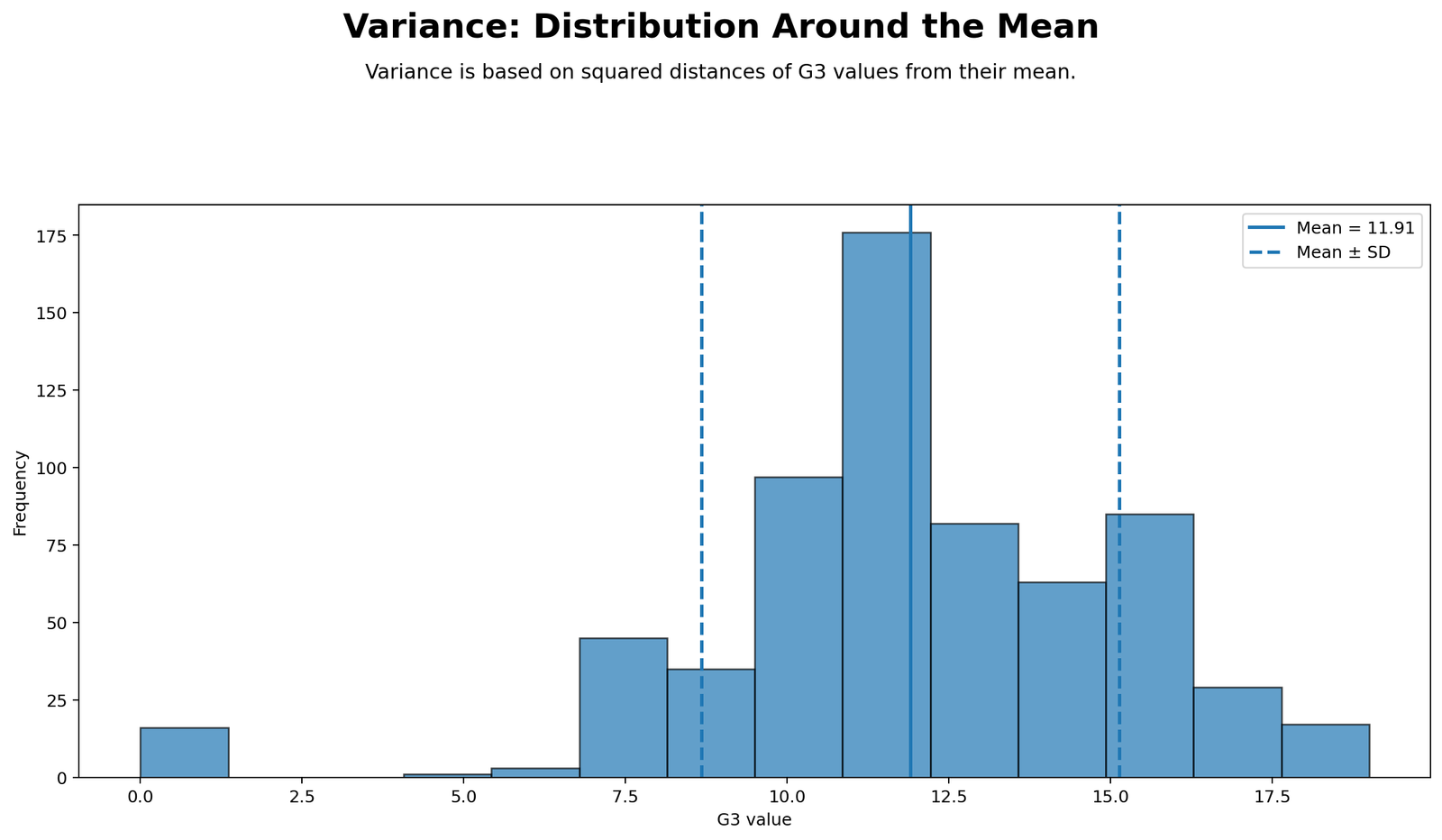
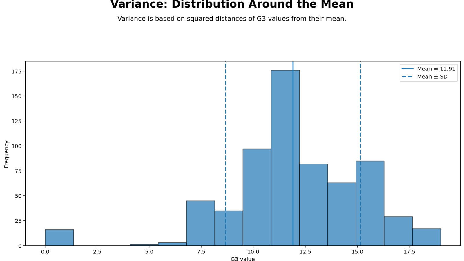
This chart explains variance visually. The solid vertical line marks the G3 mean at about 11.91. The dashed vertical lines mark approximately one standard deviation below and above the mean. Since the standard deviation is about 3.23, the dashed lines fall near 8.68 and 15.14. Most G3 values cluster around the central grade range, but there are also low scores near zero and higher scores near 18 or 19. Variance is calculated by taking the squared distance of every G3 value from the mean. Values close to 11.91 contribute little to variance, while values far from 11.91 contribute a lot. This is why the low-score values near zero strongly increase the total variance.
2. Variance: Comparison Across Numeric Variables
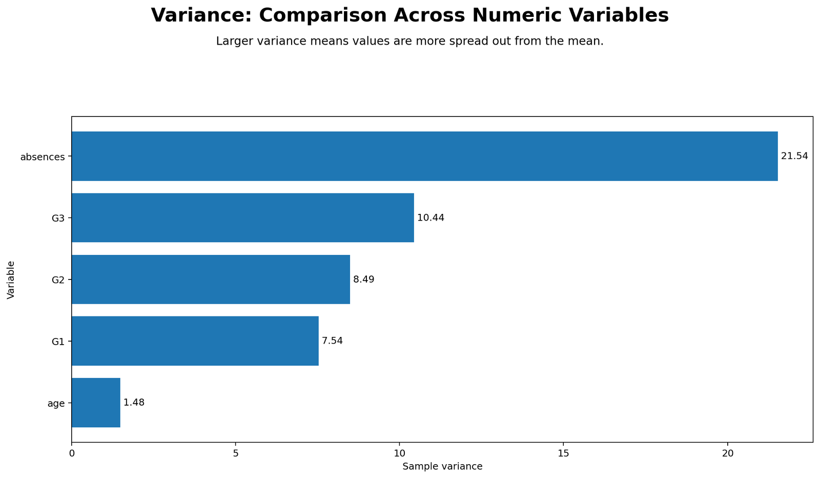
This chart ranks the selected numeric variables by sample variance. Absences has the largest variance, 21.54, which means absence counts are highly spread out. G3 has the next largest variance, 10.44, followed by G2 = 8.49 and G1 = 7.54. Age has the smallest variance, 1.48, because most students are within a narrow age range. The chart is useful because it quickly shows which variables are more dispersed. However, it should be interpreted with scale awareness: absences and grades are measured differently, so the largest variance does not automatically mean the strongest educational importance.
3. Variance and Standard Deviation
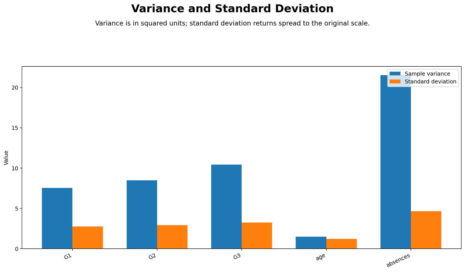
This chart compares variance with standard deviation. Variance is always in squared units, while standard deviation is the square root of variance and returns spread to the original scale. For example, G3 variance is 10.44, but its standard deviation is 3.23. Absences variance is 21.54, but its standard deviation is 4.64. This is why standard deviation is often easier to explain in reports. A standard deviation of 3.23 grade points is more understandable than a variance of 10.44 squared grade points. Still, variance is important because many statistical formulas and models are based on squared deviations.
4. Variance: Largest Squared-Deviation Contributors
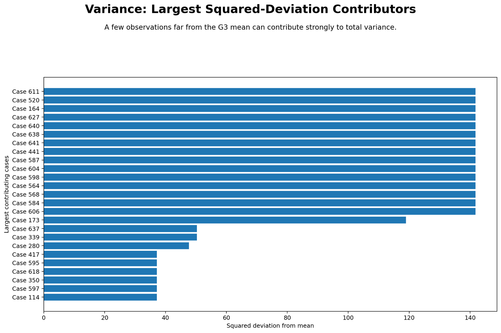
This chart shows why variance is sensitive to extreme values. Cases with G3 values far away from the mean create very large squared deviations. The largest displayed contributors have G3 = 0, a deviation of about -11.906 from the mean and a squared deviation of about 141.753. Because the deviation is squared, these cases contribute much more to total variance than scores near the mean. This does not mean the cases should automatically be deleted. Instead, it means they should be understood as important contributors to dispersion. If these values are valid grades, they are part of the real spread of the dataset.
5. Variance: Group Comparison by Sex
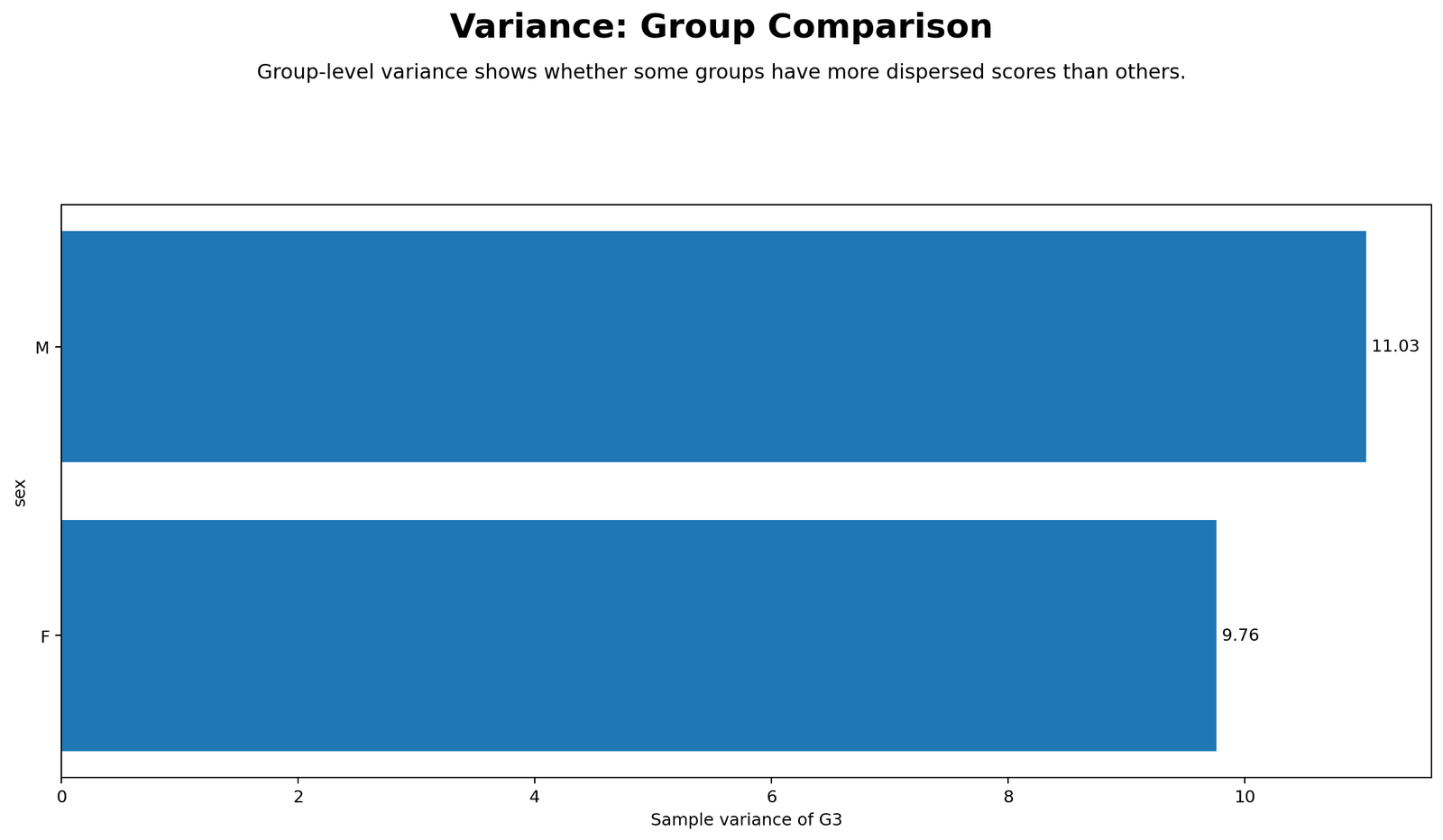
This chart compares G3 variance by sex. Female students have sample variance = 9.76, while male students have sample variance = 11.03. Descriptively, male G3 scores are slightly more spread out. Female students have a higher mean G3 score in the summary table, but variance answers a different question: it measures dispersion, not average performance. Because no formal variance equality p-value is attached, this chart should be reported as descriptive. A formal test would require Levene, Brown-Forsythe or an F-test depending on the assumptions and reporting purpose.
R Validation Charts and Interpretation
The R charts validate the same results using a different plotting style. They confirm the distribution around the mean, the ranking of variable variances, the relationship between variance and standard deviation, the influence of large squared deviations and the group-level variance comparison.
1. R Distribution Around the Mean
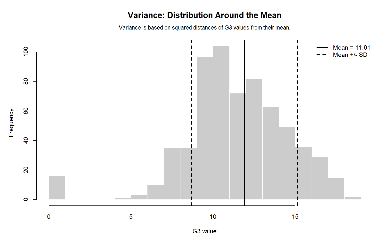
The R chart confirms that G3 scores cluster around the mean of about 11.91 but also include values far from the center. The dashed standard-deviation reference lines help readers understand how variance is connected to spread. Values outside the central range add more to total variance because their deviations from the mean are larger and then squared.
2. R Variance Comparison Across Numeric Variables
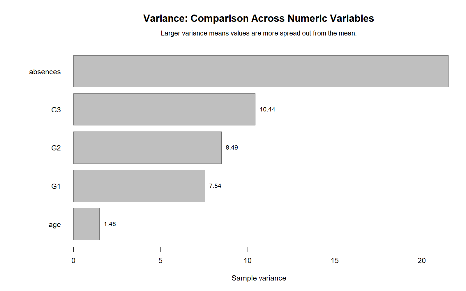
The R variance comparison confirms the Python ranking. Absences show the largest variance, followed by G3, G2, G1 and age. The chart reinforces the key result that G3 is the most variable of the three grade variables, while age is the least variable among the selected variables.
3. R Variance and Standard Deviation
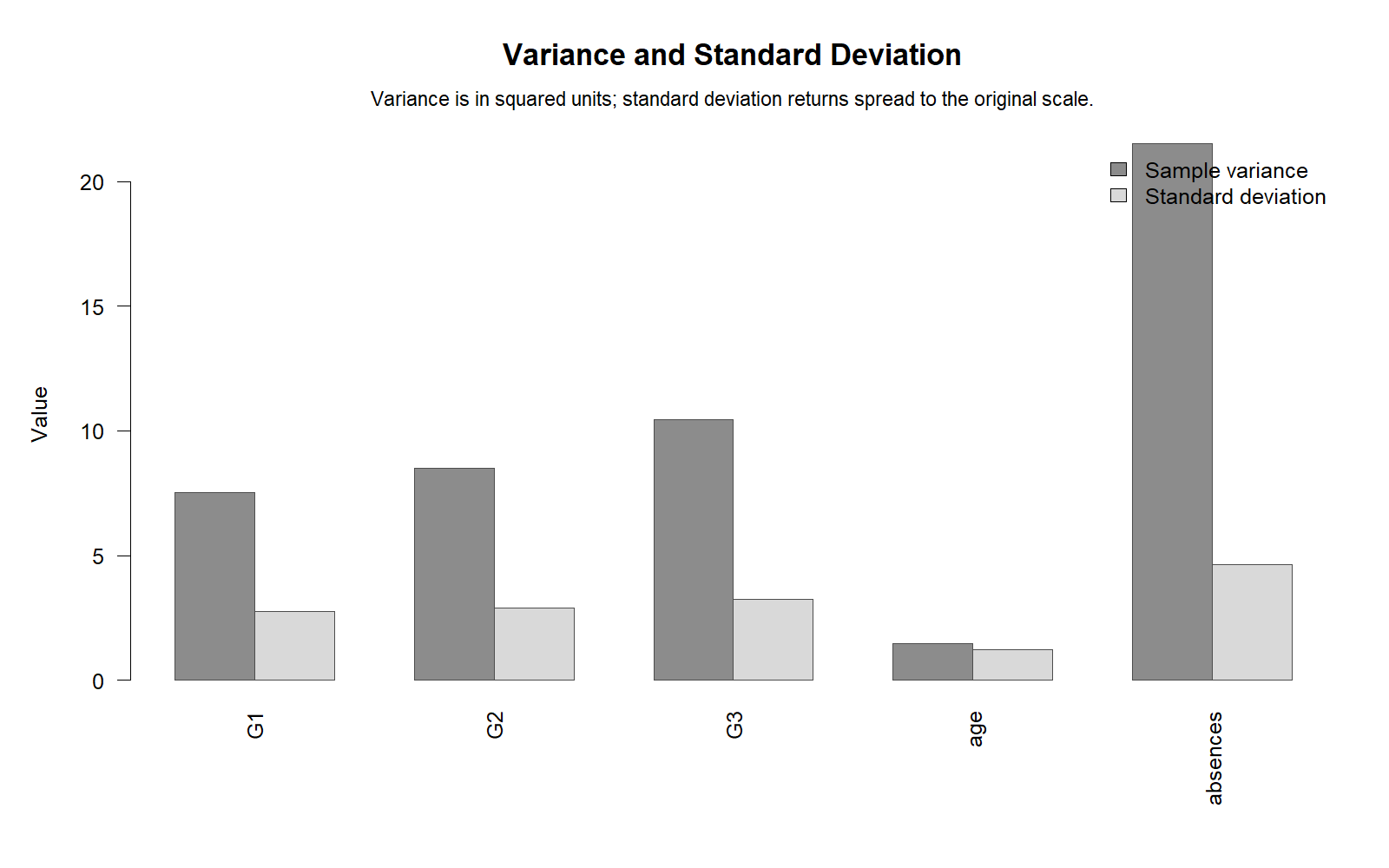
The R chart confirms that variance values are larger because they are in squared units, while standard deviation is lower because it is the square root of variance. This is an important teaching point. Variance is powerful for statistical formulas, but standard deviation is usually clearer for practical interpretation.
4. R Largest Squared-Deviation Contributors
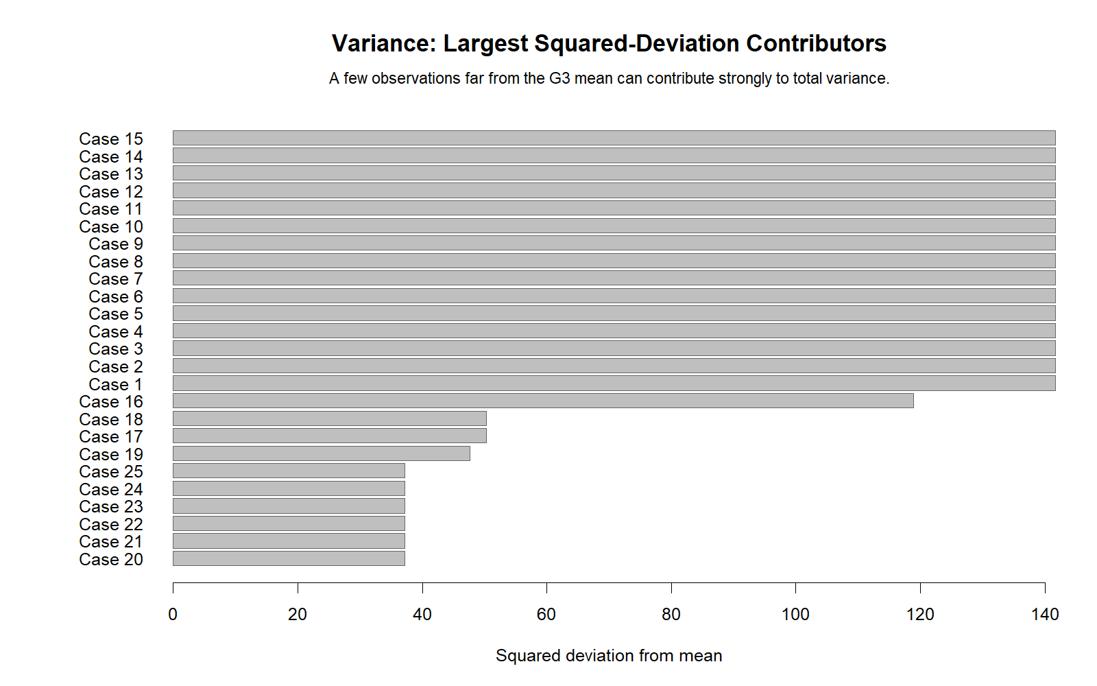
The R contributor chart confirms the same idea as the Python chart: a small number of values far from the mean can contribute strongly to total variance. Because the deviations are squared, extreme low or high values have much larger influence than values near the mean. This is why variance should be interpreted with a distribution plot or boxplot whenever possible.
5. R Group Variance Comparison
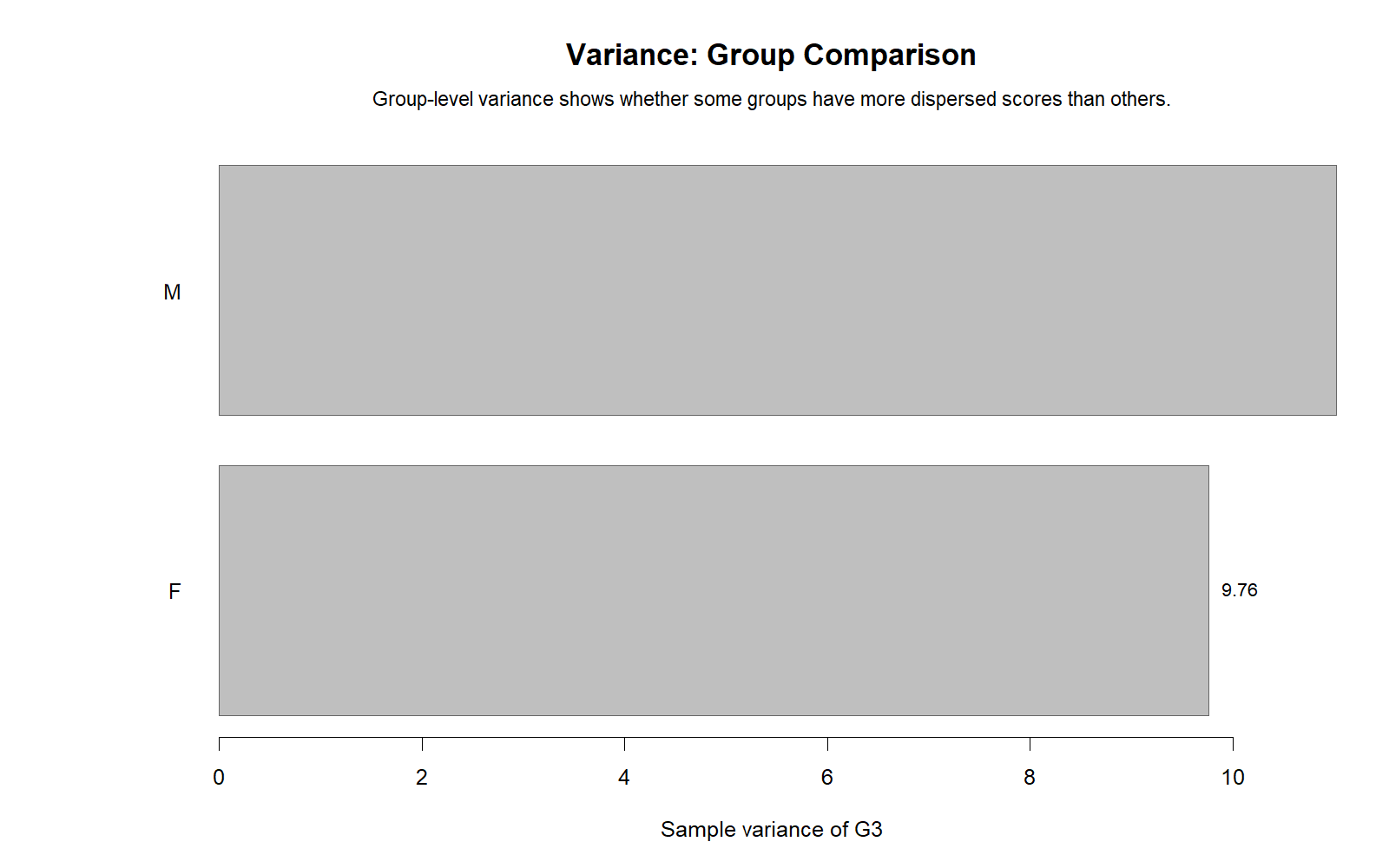
The R group comparison confirms that male students have slightly higher G3 variance than female students. This validates the descriptive group result. For formal inference, this chart should be followed by an equality-of-variance test such as Levene Test or Brown-Forsythe Test.
SPSS Output Interpretation
The SPSS output link supports the variance workflow by providing descriptive statistics and output documentation. The key values used in this guide are the sample variances, population variances, standard deviations, ranges and group-level variance summaries.
Main SPSS-Style Interpretation
For G3, the sample variance is 10.4371. This means the average squared deviation from the G3 mean is about 10.44. The standard deviation is 3.2307, which means the typical spread is about 3.23 grade points from the mean. The minimum is 0, maximum is 19 and interquartile range is 4. These values show that most grades are concentrated around the center, but a few very low scores create large squared deviations.
SPSS-Ready Reporting Table
| Measure | G3 value | SPSS-style interpretation |
|---|---|---|
| N | 649 | The variance calculation used 649 valid G3 observations. |
| Mean | 11.9060 | The average final grade is about 11.91. |
| Sample variance | 10.4371 | The average squared distance from the mean is about 10.44. |
| Population variance | 10.4211 | The population-formula variance is almost the same because N is large. |
| Standard deviation | 3.2307 | The typical spread is about 3.23 grade points. |
| Coefficient of variation | 27.13% | The standard deviation is about 27% of the mean. |
| Range | 19 | G3 scores span from 0 to 19. |
| Interquartile range | 4 | The middle 50% of G3 scores are spread across about 4 grade points. |
SPSS reporting caution: SPSS may label variance under descriptive statistics. Always check whether you are reporting sample variance or population variance. Most statistical software uses sample variance by default when calculating variance from a dataset.
How to Calculate Variance in Python, R, SPSS and Excel
Python Method
In Python, pandas calculates sample variance with var() by default because it uses ddof = 1. Population variance uses ddof = 0.
import pandas as pd
import numpy as np

df = pd.read_csv("student-por.csv", sep=";")

selected = ["G1", "G2", "G3", "age", "absences"]

summary = []
for col in selected:
    x = df[col].dropna()
    summary.append({
        "variable": col,
        "n": x.size,
        "mean": x.mean(),
        "sample_variance": x.var(ddof=1),
        "population_variance": x.var(ddof=0),
        "standard_deviation": x.std(ddof=1),
        "minimum": x.min(),
        "maximum": x.max(),
        "range": x.max() - x.min(),
        "interquartile_range": x.quantile(0.75) - x.quantile(0.25)
    })

summary_df = pd.DataFrame(summary)
print(summary_df)

# Group variance for G3 by sex
group_summary = df.groupby("sex")["G3"].agg(
    n="count",
    mean="mean",
    sample_variance=lambda s: s.var(ddof=1),
    standard_deviation=lambda s: s.std(ddof=1),
    minimum="min",
    maximum="max"
)

print(group_summary)
R Method
In R, the var() function calculates sample variance. Use a custom formula if you need population variance.
df <- read.csv("student-por.csv", sep = ";")

selected <- c("G1", "G2", "G3", "age", "absences")

variance_summary <- data.frame(
  variable = selected,
  n = sapply(df[selected], function(x) sum(!is.na(x))),
  mean = sapply(df[selected], mean, na.rm = TRUE),
  sample_variance = sapply(df[selected], var, na.rm = TRUE),
  population_variance = sapply(df[selected], function(x) {
    x <- x[!is.na(x)]
    sum((x - mean(x))^2) / length(x)
  }),
  standard_deviation = sapply(df[selected], sd, na.rm = TRUE),
  minimum = sapply(df[selected], min, na.rm = TRUE),
  maximum = sapply(df[selected], max, na.rm = TRUE)
)

variance_summary$range <- variance_summary$maximum - variance_summary$minimum

print(variance_summary)

# Group variance for G3 by sex
aggregate(G3 ~ sex, data = df, function(x) c(
  n = length(x),
  mean = mean(x),
  sample_variance = var(x),
  standard_deviation = sd(x),
  minimum = min(x),
  maximum = max(x)
))
SPSS Method
In SPSS, variance can be requested through DESCRIPTIVES, FREQUENCIES or EXAMINE. The following syntax calculates descriptive statistics for the selected variables and group summaries for G3 by sex.
DESCRIPTIVES VARIABLES=G1 G2 G3 age absences
  /STATISTICS=MEAN STDDEV VARIANCE MIN MAX.

EXAMINE VARIABLES=G3 BY sex
  /PLOT NONE
  /STATISTICS DESCRIPTIVES
  /CINTERVAL 95
  /MISSING LISTWISE
  /NOTOTAL.

OUTPUT EXPORT
  /CONTENTS EXPORT=ALL
  /PDF DOCUMENTFILE="D:\DATA ANALYSIS\A Basic Descriptive Statistics Guides\Variance\SPSS_Output\Variance-SPSS-Output.pdf".
Excel Method
Excel has direct variance formulas. Use VAR.S for sample variance and VAR.P for population variance.
| Task | Excel formula | Meaning |
|---|---|---|
| Sample variance | =VAR.S(A2:A650) | Calculates variance using n − 1. |
| Population variance | =VAR.P(A2:A650) | Calculates variance using N. |
| Standard deviation | =STDEV.S(A2:A650) | Square root of sample variance. |
| Mean | =AVERAGE(A2:A650) | Center of the distribution. |
| Squared deviation | =(A2-$B$1)^2 | Squared distance from the mean stored in B1. |
| Manual sample variance | =SUM(B2:B650)/(COUNT(A2:A650)-1) | Manual formula using squared deviations. |
How to Report Variance
Variance can be reported in a short descriptive sentence or in a table. Because variance is in squared units, it is usually helpful to report standard deviation together with variance.
Descriptive Report Example
The G3 final grade variable had a mean of 11.906, sample variance of 10.437 and standard deviation of 3.231. This indicates that G3 scores were moderately dispersed around the mean. The distribution plot showed that most values were near the center, while several very low scores contributed strongly to the total variance through large squared deviations.
Group Comparison Report Example
Descriptive group results showed that male students had slightly higher G3 variance, s² = 11.027, than female students, s² = 9.760. This suggests slightly greater dispersion in male final-grade scores. However, because no formal equality-of-variance p-value was attached, this difference should be described as a descriptive variance comparison rather than a formal hypothesis-test decision.
APA-style tip: For most student reports, write both variance and standard deviation: M = 11.91, s² = 10.44, SD = 3.23. The variance shows the statistical squared-spread measure, while the standard deviation gives the practical spread in grade points.
Common Mistakes When Interpreting Variance
| Mistake | Why it is wrong | Correct approach |
|---|---|---|
| Interpreting variance in original units | Variance is in squared units. | Use standard deviation when you want original-scale interpretation. |
| Comparing variance across different scales without caution | Variables with larger measurement scales often have larger variance. | Use coefficient of variation or standardized measures when scale differs. |
| Ignoring outliers or extreme values | Variance squares deviations, so far values strongly affect it. | Check histograms, boxplots and squared-deviation contributor charts. |
| Confusing sample and population variance | Sample variance divides by n − 1; population variance divides by N. | Report which formula was used. |
| Making a hypothesis decision without a p-value | Descriptive variance differences are not automatically statistically significant. | Use Levene, Brown-Forsythe, Cochran C or an F-test for formal variance comparison. |
Downloads and Resources
The following hosted resources support this variance guide. The chart links show the Python and R visual outputs used in the interpretation sections, and the SPSS PDF provides the software output for the variance workflow.
SPSS Output PDF
Variance SPSS output with descriptive statistics and variance results.
Python Distribution Chart
G3 distribution around the mean with mean ± standard deviation.
Python Variance Comparison Chart
Sample variance comparison across selected numeric variables.
R Group Variance Chart
R validation chart comparing G3 variance by sex.
External References
FAQs About Variance
What is variance in statistics?
Variance is a measure of spread around the mean. It is calculated by averaging squared deviations from the mean. A larger variance means values are more spread out.
What is the variance formula?
The sample variance formula is s² = Σ(xᵢ − x̄)² / (n − 1). The population variance formula is σ² = Σ(xᵢ − μ)² / N.
What is the G3 variance in this example?
The G3 final grade variable has sample variance = 10.4371, population variance = 10.4211 and standard deviation = 3.2307.
What is the difference between variance and standard deviation?
Variance is in squared units, while standard deviation is the square root of variance and is interpreted in the original measurement units. For G3, variance is 10.4371 and standard deviation is 3.2307 grade points.
Should I use sample variance or population variance?
Use sample variance when the dataset is treated as a sample from a larger population. Use population variance when the dataset is the complete population of interest. Most statistical software reports sample variance by default.
Why does absences have the largest variance?
Absences range from 0 to 32 and include many small values plus some larger values. This wider count spread creates a larger sample variance of 21.5366.
Can variance be negative?
No. Variance cannot be negative because it is based on squared deviations. The smallest possible variance is 0, which happens only when all values are the same.
How do I test whether two variances are equal?
Use a formal equality-of-variance test such as Levene Test, Brown-Forsythe Test or an F-test. In this post, female and male G3 variances are compared descriptively, but no formal p-value is attached.

