
Wald Wolfowitz Runs Test: 7 Essential Steps, Formula and Worked Example
The Wald Wolfowitz runs test is a nonparametric two-sample procedure for testing whether two independent samples come from the same continuous distribution. The samples are pooled, ordered by the outcome, converted into a sequence of group labels, and summarized by the number of label runs. This complete guide covers the Wald Wolfowitz runs test formula, exact and large-sample inference, tie handling, a verified school-grade example, interpretation, and reproducible workflows in Python, R, SPSS and Excel.
The two school grade distributions were statistically different.
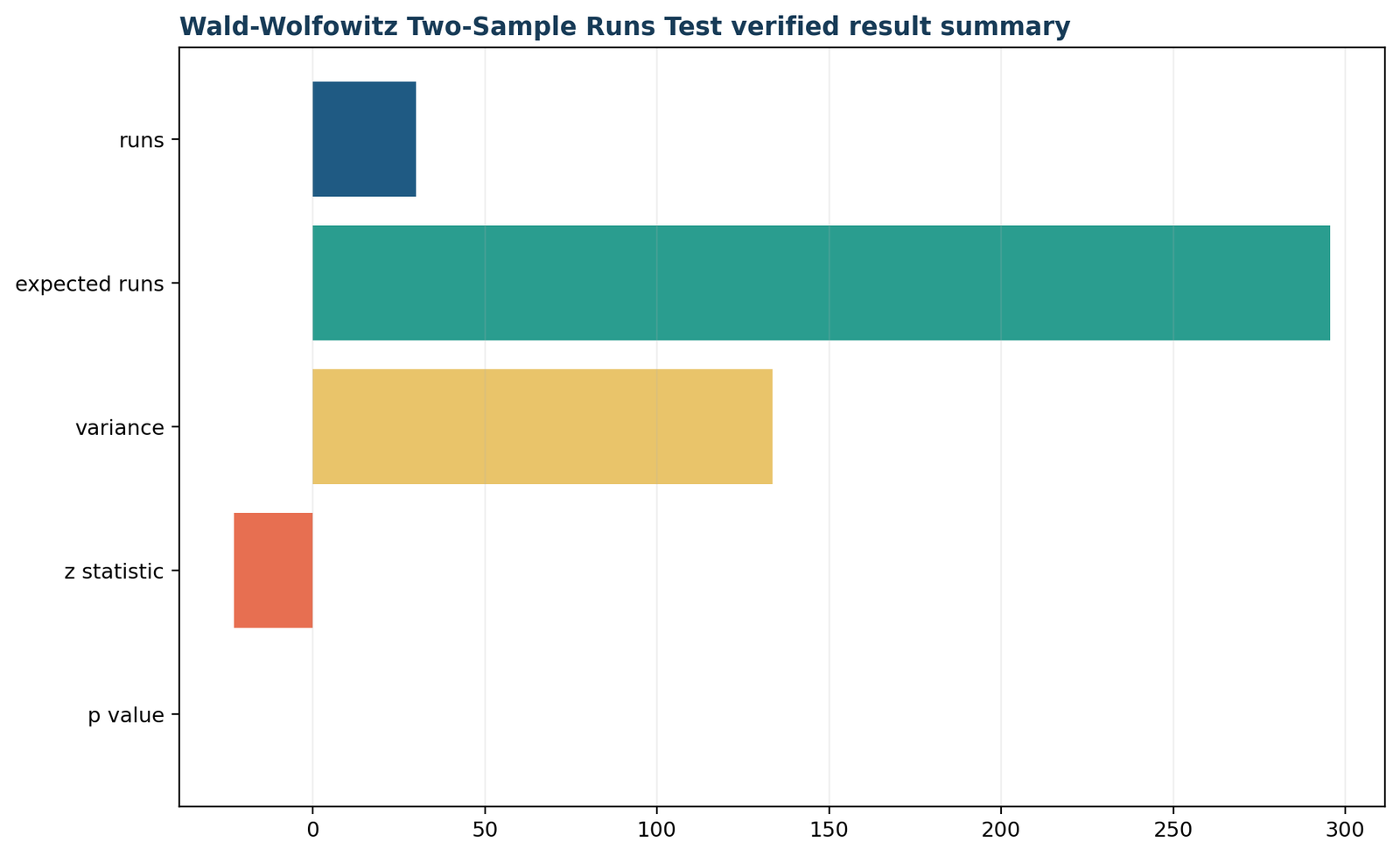
In the verified Wald Wolfowitz runs test example, final grade (G3) was compared between the GP school (n = 423) and the MS school (n = 226). After the 649 observations were pooled and sorted by G3, the stable school-label sequence contained only 30 runs. Under the null hypothesis that both samples come from the same continuous distribution, the expected number of runs was 295.600924 with variance 133.480098. The resulting statistic was z = −22.989066 and the verified two-sided probability was p = 5.99658 × 10−117.
At α = .05, the null hypothesis is rejected. The school labels are much more clustered after ordering by G3 than they would be if GP and MS had the same population distribution. GP had a higher mean grade (12.5768 versus 10.6504) and a higher median (13 versus 11), while MS had the larger standard deviation (3.8340 versus 2.6256). The Wald Wolfowitz runs test therefore detects a broad distributional difference rather than isolating only a mean, median or variance difference.
What does the Wald Wolfowitz runs test measure?
A two-sample test of complete distributional equality based on label mixing in pooled order.
The Wald Wolfowitz runs test asks whether two independent samples could reasonably have been generated by the same continuous population distribution. Unlike a test aimed only at means, medians or variances, the Wald Wolfowitz runs test can respond to differences in location, scale, shape or combinations of those features because every observation is used to create the pooled group-label sequence.
The central idea
Pool the two samples and sort the observations from smallest to largest. Replace each numerical observation by its sample label. If the two populations are identical, labels should be reasonably intermingled throughout the ordered list. If one sample tends to contain lower observations and the other tends to contain higher observations, long blocks of the same label appear and the number of runs becomes unusually small.
A run is a maximal uninterrupted block of identical labels. The sequence GP, GP, MS, MS, GP contains three runs: one GP run, one MS run and another GP run. The Wald Wolfowitz runs test converts this simple count into a probability using the sample sizes.
What a significant result means
A significant Wald Wolfowitz runs test rejects the proposition that the two complete distributions are the same. It does not, by itself, say whether the difference is specifically in the mean, median, variance, skewness or tails. Descriptive statistics, plots and targeted follow-up tests are required to characterize the pattern.
In the current analysis, GP has the higher center while MS has the greater spread. The Wald Wolfowitz runs test is appropriate as a broad equality-of-distributions test because the observed difference is not confined to one descriptive feature.
In applied work, the Wald Wolfowitz runs test should be interpreted alongside descriptive evidence. The test belongs beside other two-sample nonparametric methods such as the Mann–Whitney U test, two-sample Kolmogorov–Smirnov test, Moses test of extreme reactions and Ansari–Bradley test. The best choice depends on the scientific question.
When should you use the Wald Wolfowitz runs test?
Choose it for a broad two-distribution comparison, not merely because normality is doubtful.
Use the Wald Wolfowitz runs test when there are exactly two independent groups, the outcome can be ordered, and the null hypothesis concerns equality of the complete population distributions. The design and estimand should determine the method before software is opened.
Exactly two groups?
The classic Wald Wolfowitz runs test is a two-sample procedure.
Independent observations?
No person or unit should contribute to both samples.
Orderable outcome?
The pooled measurements must be sortable from low to high.
General difference?
The hypothesis concerns the full distributions, not only center or spread.
Ties understood?
Continuous outcomes are ideal; mixed-group ties require explicit handling.
Strong applications
Choose another method when
Wald Wolfowitz runs test calculator decision rule
A reliable Wald Wolfowitz runs test calculator must request two independent samples, pool and sort them, preserve group labels, count runs, display n1, n2, E(R), Var(R), z and the p-value, and warn when ties occur. A calculator that merely dichotomizes one sequence above and below its median is performing a one-sample runs test, not the two-sample Wald Wolfowitz runs test described here.
Wald Wolfowitz runs test assumptions: seven checks
The method is distribution-free under its null model, but not assumption-free.
The Wald Wolfowitz runs test assumptions concern sampling, independence, measurement order and ties. The usual exact distribution is cleanest for continuous populations because continuous measurements have zero probability of exact equality.
Independent samples
The two samples must be independent of each other, and observations within each sample must also be independent. Paired before-and-after data violate the design.
Random or defensible sampling
Population inference requires random sampling, random assignment or another design that supports generalization. The test cannot repair selection bias.
Orderable outcome
The outcome must have a meaningful total ordering. Numeric continuous data are ideal; sufficiently granular ordinal data may sometimes be used with careful tie treatment.
Exactly two groups
Each valid observation belongs to one and only one of two groups. More groups require a different k-sample procedure or planned pairwise tests with multiplicity control.
Continuous null model
The classic combinatorial distribution assumes no ties. With discrete scores, the test statistic depends on how opposite-group cases tied at the same value are ordered.
Missing values handled
Cases missing either the outcome or group label must be excluded consistently. Report final group sizes after exclusions.
Direction chosen in advance
Two-sided inference is the default for general distributional inequality. A one-sided low-runs alternative should be justified before inspecting results.
Review parametric versus nonparametric tests for the broader principle: “nonparametric” describes how a null distribution is obtained; it does not mean every data structure is automatically valid.
Wald Wolfowitz runs test hypotheses and data dictionary
State equality of the complete population distributions and identify the pooled ordering variable.
The Wald Wolfowitz runs test uses a broader null hypothesis than a two-sample location or scale test. The null says that GP and MS final grades follow the same population distribution; the alternative says that the distributions differ in at least one respect.
Formal hypotheses
The cumulative distribution functions are identical across the full grade scale.
The two distributions differ in location, spread, shape, tails or a combination of these characteristics.
The observed run count is the test statistic. Too few runs indicate that labels cluster in different portions of the pooled ordering. Depending on the alternative and implementation, unusually many runs can also be treated as evidence against random mixing.
Variables and coding
Two-sided research wording
Null: GP and MS students have the same population distribution of final grades.
Alternative: the population distribution of final grades differs between GP and MS students.
This wording is preferable to “the medians are equal,” because the Wald Wolfowitz runs test is not limited to medians.
Observed descriptive pattern
GP has a higher mean and median, whereas MS has greater standard deviation and IQR. These simultaneous differences motivate a general distributional test. They also show why a significant Wald Wolfowitz runs test should not be reduced to a single statement about average grades.
Wald Wolfowitz runs test formula, expectation and exact distribution
Count label blocks, then compare the count with its combinatorial null distribution.
The Wald Wolfowitz runs test formula uses the observed number of runs R and the two sample sizes. For large samples, R is standardized with its null mean and variance. For small tie-free samples, the exact probability can be calculated from combinations.
Step 1: define and count runs
After pooling and sorting, let Li be the group label at ordered position i. The first observation begins a run. Every later position begins a new run when its label differs from the preceding label.
I(·) equals 1 when a label change occurs and 0 otherwise.
Step 2: null expectation
When labels are randomly interspersed, the expected run count increases with the balance and size of the two samples.
Step 3: null variance
The standard deviation is √Var(R). This formula applies to the usual tie-free two-sample labeling model.
Step 4: large-sample statistic
For the current large sample, no continuity correction is needed to reproduce the supplied verified result. A two-sided probability is calculated as 2Φ(−|z|).
Exact probability when R is even
There are k runs from each sample, and the sequence may begin with either sample.
Exact probability when R is odd
One sample contributes k+1 runs and the other contributes k runs.
| Current calculation | Formula substitution | Result |
|---|---|---|
| Expected runs | 1 + 2(423)(226)/649 | 295.600924499 |
| Variance | 2(423)(226)[2(423)(226)−649] / [649²(648)] | 133.480098443 |
| Standard deviation | √133.480098443 | 11.553358752 |
| z statistic | (30−295.600924499)/11.553358752 | −22.989065795 |
| Two-sided p | 2Φ(−|−22.989065795|) | 5.996580928 × 10−117 |
Wald Wolfowitz runs test example: GP versus MS final grades
A complete example with 649 school records, pooled ordering and descriptive context.
This Wald Wolfowitz runs test example compares final-grade distributions between two schools. It preserves the exact source-group sizes, shows how runs arise, reports the full calculation, and separates the stable-order result from the additional tie-order sensitivity audit.
Research scenario
The dataset contains final grade G3 and school membership. There are 423 GP observations and 226 MS observations. The research question is whether the entire final-grade distribution is the same for the two schools.
GP grades are more concentrated in the higher central range, while MS includes more very low grades and a wider spread. When all observations are sorted by grade, this pattern produces long school-specific blocks. The Wald Wolfowitz runs test summarizes the amount of mixing through R.
Group descriptives
| Statistic | GP | MS |
|---|---|---|
| n | 423 | 226 |
| Mean | 12.5768 | 10.6504 |
| Median | 13 | 11 |
| SD | 2.6256 | 3.8340 |
| Q1 | 11 | 9 |
| Q3 | 14 | 13 |
| IQR | 3 | 4 |
| Range | 0–19 | 0–19 |
How the pooled sequence begins
The stable grade ordering starts with the following school labels. Vertical bars mark new runs:
G3 = 0: GP | MS MS MS MS MS MS MS MS MS MS MS MS MS MS
G3 = 1: | GP
G3 = 5: GP
G3 = 6: GP GP | MS
G3 = 7: | GP GP GP | MS MS MS MS MS MS MS
G3 = 8: | GP × 14 | MS × 21
As the grades continue, most tied grade blocks contain a GP block followed by an MS block. The full stable ordering yields 30 runs. The longest run contains 70 GP observations at G3 = 11; the sequence has median run length 14.5 and mean run length 21.63.
| G3 | GP count | MS count | Pooled count | Distributional signal |
|---|---|---|---|---|
| 0 | 1 | 14 | 15 | Most zero grades are in MS. |
| 8 | 14 | 21 | 35 | MS is more represented at this lower grade. |
| 9 | 10 | 25 | 35 | MS is more represented. |
| 10 | 53 | 44 | 97 | Both groups are common. |
| 11 | 70 | 34 | 104 | Largest pooled frequency; GP dominates. |
| 13 | 67 | 15 | 82 | GP is strongly represented. |
| 15 | 41 | 8 | 49 | GP dominates the higher grade. |
| 17 | 24 | 5 | 29 | GP remains more represented. |
Wald Wolfowitz runs test statistics, result and tie-order audit
The stable-order result is extreme, and the conclusion survives every possible tie arrangement.
The Wald Wolfowitz runs test statistics show an enormous departure from equal distributional mixing. The observed R is 265.6009 runs below its null expectation, equivalent to 22.9891 null standard deviations.
Primary inference
Reject H0
The two-sided probability is effectively zero for ordinary reporting precision, but it is not mathematically equal to zero. GP and MS do not show the label mixing expected under identical final-grade distributions.
Calculation audit
Exhaustive tie-order sensitivity
Within a grade value shared by both schools, the order of GP and MS labels is not determined by G3. A dynamic-programming audit was therefore used to find the minimum and maximum number of runs that can be created while keeping every observation at its original grade.
| Tie arrangement | Runs | z | Two-sided p | Decision |
|---|---|---|---|---|
| Minimum possible mixing | 16 | −24.2008 | 2.18 × 10−129 | Reject H0 |
| Supplied stable order | 30 | −22.9891 | 5.9966 × 10−117 | Reject H0 |
| Maximum possible mixing | 378 | 7.1320 | 9.89 × 10⁻¹³ | Reject H0 |
The maximum possible run count exceeds the null expectation and is significant in the opposite direction. Therefore, every allowable within-grade order is inconsistent with the ordinary equal-distributions reference model at α = .05. This does not remove the discrete-data limitation, but it demonstrates that the decision is not an artifact of choosing GP before MS within tied grade blocks.
Wald Wolfowitz runs test in Python: verified calculation and charts
Reproduce the workbook directly, then cross-check with statsmodels.
The Wald Wolfowitz runs test Python workflow below preserves group labels, uses a stable sort for the supplied result, calculates R from label changes and avoids p-value cancellation. The statsmodels implementation provides a useful cross-check and issues a tie warning.
import numpy as np
import pandas as pd
from scipy.stats import norm# Required columns: school and G3
df = pd.read_csv("dataset.csv")[["school", "G3"]].dropna()
df = df[df["school"].isin(["GP", "MS"])].copy()
# Stable pooled ordering reproduces the supplied workbook sequence.
pooled = df.sort_values("G3", kind="mergesort").reset_index(drop=True)
labels = pooled["school"].to_numpy()
runs = 1 + np.sum(labels[1:] != labels[:-1])
n_gp = np.sum(labels == "GP")
n_ms = np.sum(labels == "MS")
N = n_gp + n_ms
expected = 1 + (2 * n_gp * n_ms) / N
variance = (
2 * n_gp * n_ms * (2 * n_gp * n_ms - N)
/ (N**2 * (N - 1))
)
z = (runs - expected) / np.sqrt(variance)
# Numerically stable for a very large absolute z statistic.
p_two_sided = 2 * norm.cdf(-abs(z))
print(f"Runs = {runs}")
print(f"Expected runs = {expected:.12f}")
print(f"Variance = {variance:.12f}")
print(f"z = {z:.12f}")
print(f"Two-sided p = {p_two_sided:.12e}")
from statsmodels.sandbox.stats.runs import runstest_2sampgp = df.loc[df["school"].eq("GP"), "G3"].to_numpy()
ms = df.loc[df["school"].eq("MS"), "G3"].to_numpy()
z_sm, p_sm = runstest_2samp(gp, ms, correction=False)
print(z_sm, p_sm)
# -22.989065795455694, 5.996580928044667e-117
The statsmodels function is located in a sandbox module and explicitly warns that the two-sample procedure is intended for continuous distributions. For mixed-group ties, its documented tie rule is not the same as an exhaustive maximum/minimum-run analysis. The post therefore reports both the software cross-check and the separate tie-range audit.
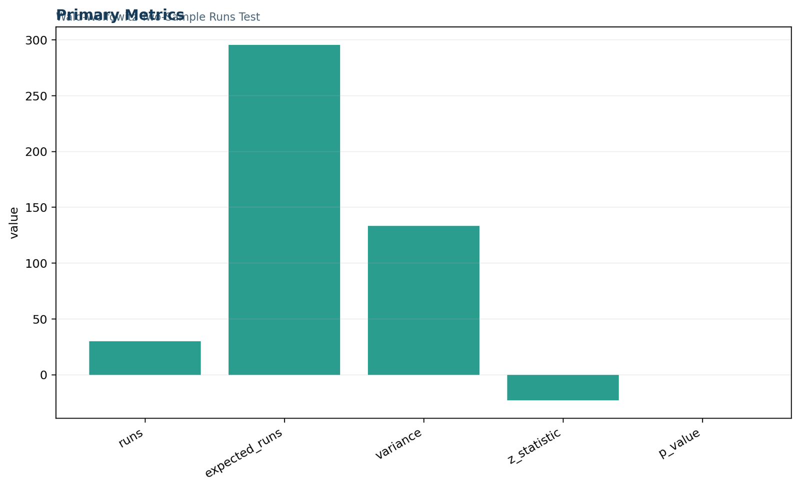
Python chart 1: Primary metrics
The first chart places the observed run count beside its null expectation, variance, z statistic and p-value. The defining contrast is 30 observed runs versus 295.6009 expected runs. The z statistic is −22.9891, so the observed school labels are far more clustered in the pooled grade ordering than the equal-distribution null predicts.
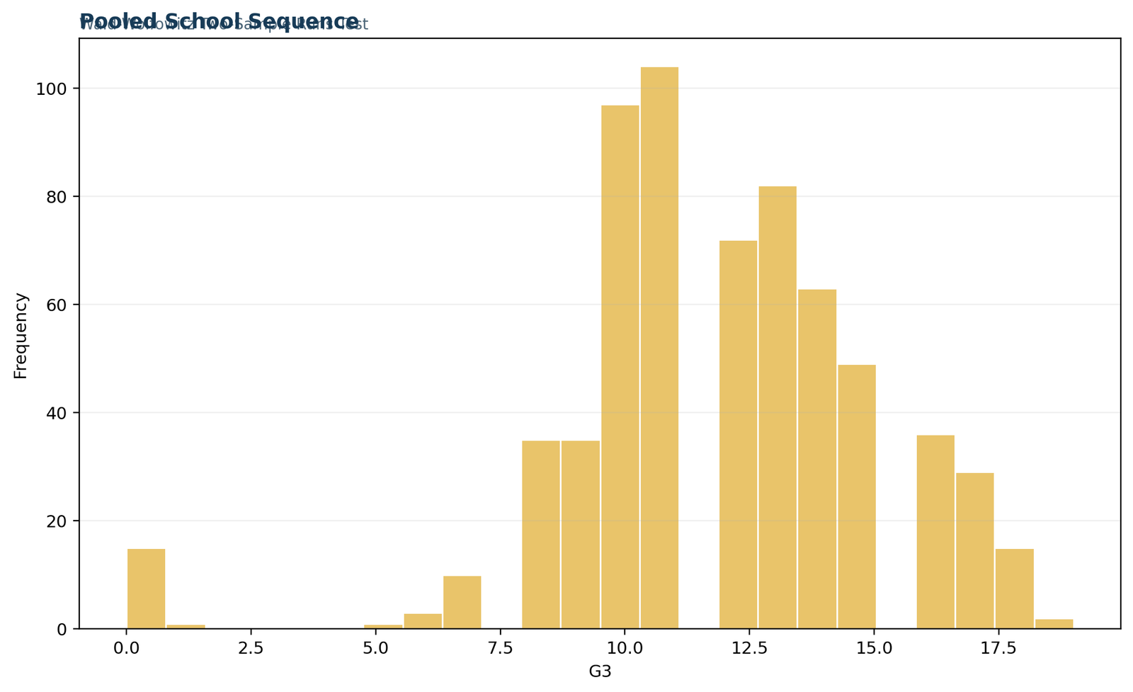
Python chart 2: Pooled school sequence
The pooled G3 values are ordered from the smallest grade to the largest grade, and school membership is then read along that ordering. The grade frequencies peak around 10 and 11. Because GP and MS cases tend to occupy different portions of the grade scale, labels remain together for long stretches instead of alternating at the rate expected when both schools have the same distribution.
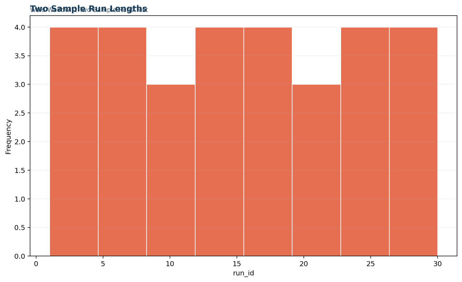
Python chart 3: Run-index profile
This panel groups the 30 identified run IDs into bins. Because its horizontal axis is the run identifier rather than the actual run length, it is best interpreted as confirmation of the 30-run structure. The underlying stable-order sequence has run lengths from 1 to 70 cases, a median run length of 14.5 and a mean of 21.63.
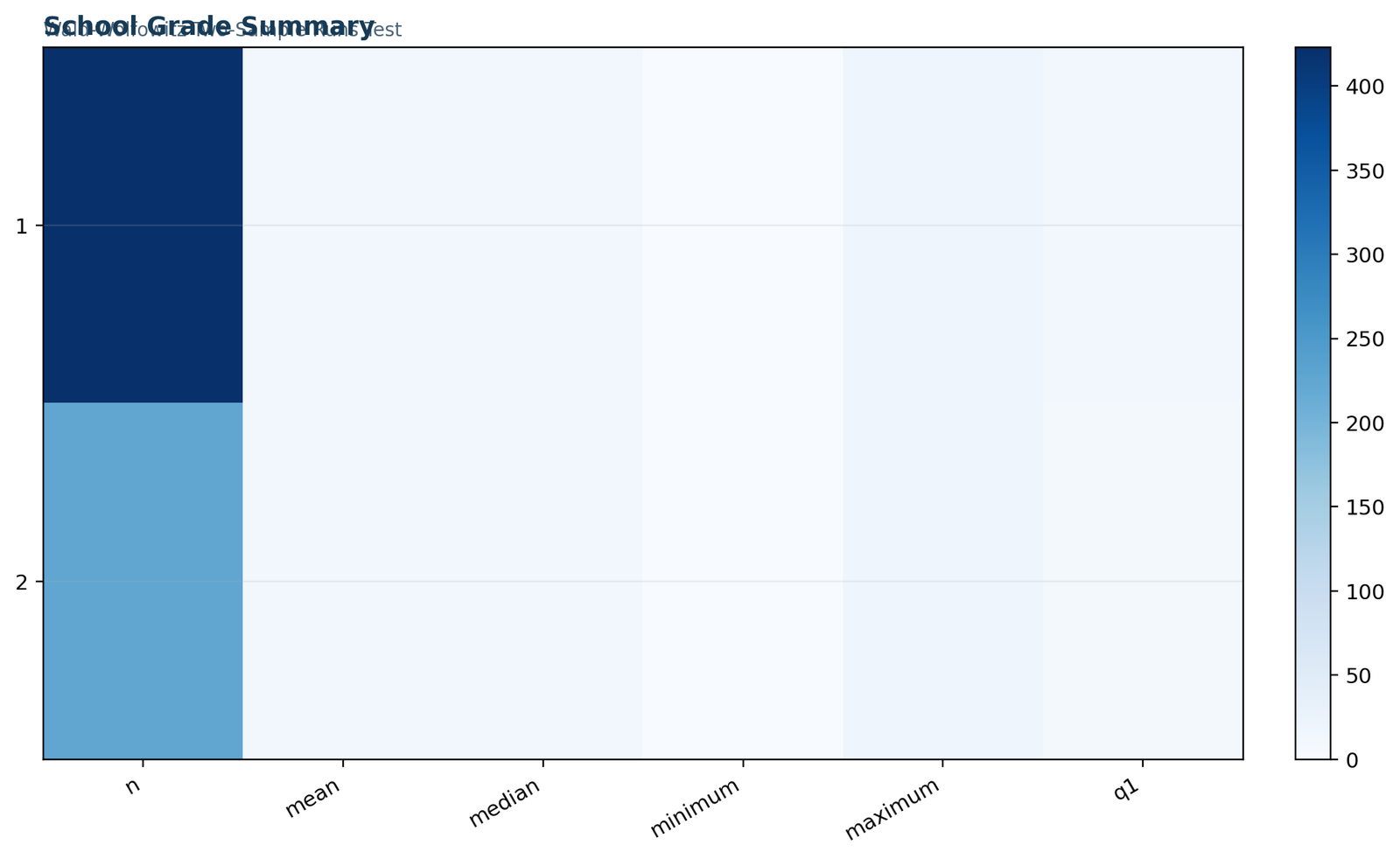
Python chart 4: School grade summary
The two-row summary compares school-specific sample size, mean, median, minimum, maximum and first quartile. GP contributes 423 cases with mean G3 = 12.5768 and median 13; MS contributes 226 cases with mean G3 = 10.6504 and median 11. The location and spread differences help explain why the pooled labels form unusually long blocks.
Python chart 5: Verified result summary
The final verification chart repeats the calculation on a common horizontal scale: R = 30, E(R) = 295.6009, Var(R) = 133.4801, z = −22.9891 and p = 5.9966 × 10⁻¹¹⁷. The p-value appears visually at zero because it is tiny relative to the other metrics, not because the mathematical probability is exactly zero.
Wald Wolfowitz runs test in R: DescTools and manual verification
Use a dedicated two-sample function and show the underlying run calculation.
The Wald Wolfowitz runs test in R can be performed with DescTools::RunsTest() when two numeric vectors are supplied. A manual calculation is still valuable because it documents the exact pooled order and connects the software output to R, E(R), Var(R) and z.
df <- read.csv("dataset.csv")
df <- na.omit(df[c("school", "G3")])
df <- df[df$school %in% c("GP", "MS"), ]# Stable ordering by G3.
ord <- order(df$G3, method = "radix")
pooled <- df[ord, ]
lab <- pooled$school
R_obs <- 1 + sum(lab[-1] != lab[-length(lab)])
n_gp <- sum(lab == "GP")
n_ms <- sum(lab == "MS")
N <- n_gp + n_ms
E_R <- 1 + 2 * n_gp * n_ms / N
Var_R <- 2 * n_gp * n_ms * (2 * n_gp * n_ms - N) /
(N^2 * (N - 1))
z <- (R_obs - E_R) / sqrt(Var_R)
p_two <- 2 * pnorm(-abs(z))
c(runs = R_obs, expected = E_R, variance = Var_R,
z = z, p_value = p_two)
library(DescTools)gp <- df$G3[df$school == "GP"]
ms <- df$G3[df$school == "MS"]
RunsTest(gp, ms,
alternative = "two.sided",
exact = FALSE,
correct = FALSE)
runs.test implement only a one-sample randomness test. Supplying two numeric vectors to DescTools::RunsTest() requests the two-sample Wald Wolfowitz runs test. Confirm the method name printed in the returned object.R chart 1: Primary metrics
The first chart places the observed run count beside its null expectation, variance, z statistic and p-value. The defining contrast is 30 observed runs versus 295.6009 expected runs. The z statistic is −22.9891, so the observed school labels are far more clustered in the pooled grade ordering than the equal-distribution null predicts.
R chart 2: Pooled school sequence
The pooled G3 values are ordered from the smallest grade to the largest grade, and school membership is then read along that ordering. The grade frequencies peak around 10 and 11. Because GP and MS cases tend to occupy different portions of the grade scale, labels remain together for long stretches instead of alternating at the rate expected when both schools have the same distribution.
R chart 3: Run-index profile
This panel groups the 30 identified run IDs into bins. Because its horizontal axis is the run identifier rather than the actual run length, it is best interpreted as confirmation of the 30-run structure. The underlying stable-order sequence has run lengths from 1 to 70 cases, a median run length of 14.5 and a mean of 21.63.
R chart 4: School grade summary
The two-row summary compares school-specific sample size, mean, median, minimum, maximum and first quartile. GP contributes 423 cases with mean G3 = 12.5768 and median 13; MS contributes 226 cases with mean G3 = 10.6504 and median 11. The location and spread differences help explain why the pooled labels form unusually long blocks.
R chart 5: Verified result summary
The final verification chart repeats the calculation on a common horizontal scale: R = 30, E(R) = 295.6009, Var(R) = 133.4801, z = −22.9891 and p = 5.9966 × 10⁻¹¹⁷. The p-value appears visually at zero because it is tiny relative to the other metrics, not because the mathematical probability is exactly zero.
Wald Wolfowitz runs test in SPSS: menu, syntax and ties
SPSS provides the dedicated procedure through its legacy two-independent-samples dialog.
The Wald Wolfowitz runs test SPSS workflow is available under the two-independent-samples legacy procedures. SPSS pools and ranks the outcome, performs a runs test using group membership, and provides special minimum/maximum calculations when tied outcome values contain both groups.
SPSS menu steps
What to inspect
Verify the valid counts for both groups, the reported number of runs, z and the significance label. When ties occur across groups, SPSS can report minimum and maximum possible runs and corresponding statistics. This is especially relevant for integer grades.
The public report should state whether the displayed probability is one-tailed or two-tailed. The worked workbook uses the two-sided normal probability based on z = −22.9891.
* Recode string school if a numeric grouping variable is required.

AUTORECODE VARIABLES=school /INTO school_num.

VALUE LABELS school_num 1 'GP' 2 'MS'.NPAR TESTS

/W-W = G3 BY school_num(1 2)

/STATISTICS = DESCRIPTIVES QUARTILES

/MISSING ANALYSIS.
Wald Wolfowitz runs test Excel calculation
Build an auditable pooled sequence and use a numerically stable probability formula.
A correct Wald Wolfowitz runs test Excel workbook must keep raw input separate from the ordered working table. The supplied workbook does this with Data_Input, Working, Calculations, Diagnostics and Reporting sheets.
Recommended columns and formulas
| Location | Purpose | Formula or action |
|---|---|---|
| Working A | Sequence position | 1 through N after sorting G3 ascending. |
| Working B | Observed G3 | Copy the pooled sorted outcome. |
| Working C | School label | Carry GP or MS with each observation. |
| Working D5 | First run start | =1 |
| Working D6 downward | Later run starts | =--(C6<>C5) |
| Runs | Observed R | =SUM(Working!D5:D653) |
| Expected | E(R) | =1+2*n1*n2/N |
| Variance | Var(R) | =2*n1*n2*(2*n1*n2-N)/(N^2*(N-1)) |
| z | Standardized statistic | =(Runs-Expected)/SQRT(Variance) |
| p-value | Stable two-sided probability | =2*NORM.S.DIST(-ABS(z),TRUE) |
Why the workbook displayed zero
The expression =2*(1-NORM.S.DIST(ABS(z),TRUE)) first asks Excel for a cumulative probability so close to 1 that it rounds to exactly 1. Subtracting that rounded value from 1 returns zero. This is numerical cancellation.
The lower-tail equivalent =2*NORM.S.DIST(-ABS(z),TRUE) evaluates the tiny tail directly and preserves the verified value, approximately 5.9966 × 10−117.
Handling ties in Excel
A single stable sort produces one allowable sequence, not a unique tie-free answer. At minimum, flag every G3 value containing both schools. For a rigorous audit, calculate minimum and maximum attainable runs within tied blocks or reproduce SPSS’s tie-range output.
Never break ties by sorting on group and then present that arrangement as if it were determined by the outcome. State the secondary sort rule.
Wald Wolfowitz runs test in MATLAB, SAS and Stata
Distinguish genuine two-sample implementations from one-sample randomness commands.
Searches for a Wald Wolfowitz runs test MATLAB, SAS or Stata command often lead to one-sample runs procedures. A software function named “runstest” is not automatically the two-sample Wald Wolfowitz runs test.
MATLAB
MATLAB’s built-in runstest tests randomness in one observed sequence using values above/below a reference or runs up/down. It is not the pooled two-sample equality-of-distributions procedure. For the current analysis, implement the pooled-label algorithm directly using sortrows, label changes and the formulas shown above.
T = table(G3, school);

T = sortrows(T, 'G3');

lab = string(T.school);

R = 1 + sum(lab(2:end) ~= lab(1:end-1));
SAS
A dependable SAS workflow can sort the pooled data by G3, retain group membership, count changes in a DATA step and calculate the large-sample statistic. Because ties require special treatment, compare the custom sequence with an implementation that documents minimum and maximum possible runs rather than relying on an unrelated one-sample randomness option.
proc sort data=grades out=pooled;

by G3;

run;data runs;

set pooled;

retain R 0 previous '';

if _N_=1 or school ne previous then R+1;

previous=school;

run;
Stata
Stata commands found for runs above/below a median typically address one-sample randomness. A transparent two-sample analysis can be programmed after sorting by G3 and counting school-label changes. Document the sort rule, especially within ties, and verify the result with SPSS, Python or R.
Wald Wolfowitz runs test versus alternative nonparametric tests
Match the procedure to the difference that matters scientifically.
The Wald Wolfowitz runs test is a broad distributional test, but it is not uniformly the most powerful procedure for every alternative. A targeted test is often preferable when the research question concerns only location or only scale. The Wald Wolfowitz runs test is most defensible when the complete distribution is the stated target.
| Method | Primary null | Best suited to | Main caution |
|---|---|---|---|
| Wald Wolfowitz runs test | Two complete distributions are equal. | General location, scale or shape differences that create label clustering. | Ties make pooled order nonunique; power depends on the alternative. |
| Mann–Whitney U | Equal relative ordering / distributions; location under equal shape. | Systematic upward or downward shift. | Location interpretation needs comparable shape. |
| Two-sample K–S | Equal continuous distributions. | Maximum CDF separation anywhere on the scale. | Classical calibration is affected by ties and discrete outcomes. |
| Ansari–Bradley | Equal scale under common location and shape. | Two-sample dispersion differences. | Location differences contaminate scale interpretation. |
| Moses extreme reactions | Equal variability / extreme reaction pattern. | Robust scale comparison. | Block construction and interpretation differ from runs. |
| Two-sample t test | Equal population means. | Mean differences with suitable sampling conditions. | Does not test complete distributional equality. |
| One-sample runs test | Sequence order is random. | Temporal or ordered randomness around a cutoff. | Not a two-sample distribution comparison. |
Diagnostics, tie checks and common Wald Wolfowitz mistakes
Validate the sequence before interpreting its p-value.
A defensible Wald Wolfowitz runs test procedure includes more than counting labels. Every Wald Wolfowitz runs test should preserve an auditable pooled sequence. The analyst should audit group coding, sorted values, tie blocks, run starts, tail calculation and the exact test name used by software.
Pre-analysis diagnostics
Calculation diagnostics
| Common mistake | Why it is wrong | Better practice |
|---|---|---|
| Using a one-sample runs command | It tests sequence randomness, not equality of two distributions. | Confirm the method explicitly accepts two samples or a group indicator. |
| Calling the test a median test | It can respond to location, scale and shape differences. | State equality of complete distributions. |
| Ignoring ties | Opposite-group cases with equal values can be ordered in multiple ways. | Use documented tie handling and report sensitivity. |
| Reporting p = 0 | Finite test statistics do not produce an exact probability of zero. | Report p < .001 or scientific notation. |
| Interpreting significance as causation | School membership may reflect many confounding characteristics. | Use associational language unless the design supports causality. |
| Skipping descriptive plots | The runs test does not identify the type or direction of difference. | Report group summaries and distribution plots. |
How to report the Wald Wolfowitz runs test in APA style
Report the groups, ordering variable, run count, reference method, z, p and tie treatment.
An APA-style Wald Wolfowitz runs test report should describe the complete-distribution hypothesis and avoid claiming that the test specifically proves a mean or median difference.
Concise APA-style result
A Wald Wolfowitz two-sample runs test indicated that the distribution of final grades differed between GP (n = 423) and MS (n = 226), R = 30, E(R) = 295.60, z = −22.99, p < .001. GP had a higher median grade (Mdn = 13) than MS (Mdn = 11), whereas MS showed greater variability (SD = 3.83 versus 2.63). Because G3 contained extensive ties, the stable-order result was supplemented by a possible-run sensitivity analysis; all allowable run counts remained significant.
Full methods wording
“The two independent school samples were pooled and ordered by final grade. School membership was converted into a binary label sequence, and a run was defined as a maximal block of identical consecutive labels. The observed number of runs was standardized using the large-sample Wald Wolfowitz expectation and variance. A two-sided normal probability was used. Because the integer-valued outcome produced mixed-group ties, minimum and maximum possible runs were also evaluated.”
Interpretation wording
“The rejection indicates that the two samples are not consistent with the same complete grade distribution. Descriptive statistics suggest that GP grades are higher in location, whereas MS grades are more variable. The test does not isolate a single distributional parameter and does not establish a causal school effect.”
Wald Wolfowitz runs test PDF, Excel and software downloads
Use the reports to audit code, output and the worked calculation.
The supplied Wald Wolfowitz runs test PDF files and Excel workbook reproduce the same school-grade analysis. The downloadable materials should be used together: the reports show software output and the workbook exposes row-level formulas.
Python report PDFVerified Python calculation, charts and result summary.Download PDF →
R report PDFR workflow and matching run-test results.Download PDF →
SPSS output PDFTwo-independent-samples output and diagnostics.Download PDF →
Worked Excel analysisRaw data, pooled sequence, formulas and verification sheet.Download workbook →
Official Wald Wolfowitz references and software documentation
Method identity and software behavior were checked against primary documentation.
The Wald Wolfowitz runs test was introduced as a two-sample nonparametric test of whether two samples come from the same population. Modern software documentation differs in exact small-sample, correction and tie behavior, so the implementation must be named in reproducible reports.
Wald Wolfowitz runs test FAQs
Answers to the most common formula, software, tie and interpretation questions.
What is the Wald Wolfowitz runs test?
The Wald Wolfowitz runs test is a nonparametric test for whether two independent samples come from the same continuous distribution. It pools and orders the measurements, converts them to sample labels and counts consecutive label runs.
What is a run in the Wald Wolfowitz test?
A run is a maximal consecutive block of the same group label. In A A B B A, there are three runs: A A, B B and A.
What does a small number of runs indicate?
Too few runs indicate that labels cluster in different portions of the pooled ordering. This is evidence that the samples may not come from the same distribution.
What is the Wald Wolfowitz runs test formula?
The large-sample mean is E(R) = 1 + 2n₁n₂/N, and the variance is 2n₁n₂(2n₁n₂ − N)/[N²(N − 1)]. The standardized statistic is z = [R − E(R)]/√Var(R).
Is the Wald Wolfowitz test the same as a one-sample runs test?
No. The two-sample test orders pooled observations and examines sample labels. A one-sample runs test examines randomness in one sequence relative to a cutoff.
Is it a test of medians?
No. The null concerns equality of complete distributions. A result can be caused by location, spread, shape or tail differences.
How many groups can be compared?
The classic procedure compares exactly two independent samples. More than two groups require another method or planned pairwise analyses with multiplicity control.
Can the Wald Wolfowitz runs test handle ties?
The classic exact theory assumes continuous distributions and no ties. Software may report minimum and maximum possible runs or apply a documented tie rule. The chosen approach must be reported.
Why are ties important in the school example?
G3 has only 17 observed values, so many GP and MS observations share the same grade. Their order within a tied grade is not determined by G3 and can change R.
Does tie order change the conclusion here?
No. The possible run count ranges from 16 to 378, and even the maximum-run arrangement gives a highly significant two-sided result.
How is the test performed in Python?
Use statsmodels runstest_2samp for a cross-check or manually sort the pooled values, count label changes and apply the expectation and variance formulas. Inspect tie behavior explicitly.
How is the test performed in R?
DescTools::RunsTest(x, y) performs the two-sample Wald Wolfowitz test. A manual pooled-order calculation can verify the printed output.
Where is the test in SPSS?
Use Analyze → Nonparametric Tests → Legacy Dialogs → 2 Independent Samples and select Wald Wolfowitz runs, or use the NPAR TESTS W-W subcommand.
Why does Excel show p = 0?
The upper-tail subtraction formula loses precision when the normal CDF rounds to 1. Use =2*NORM.S.DIST(-ABS(z),TRUE) to evaluate the tiny lower tail directly.
What result was obtained in the worked example?
The supplied stable ordering produced R = 30, E(R) = 295.6009, z = −22.9891 and p = 5.9966 × 10⁻¹¹⁷.
How should the result be interpreted?
The GP and MS final-grade samples are inconsistent with the same population distribution. GP has a higher center, while MS has greater spread. The test does not establish causality.
Should an effect size be reported?
There is no single universally accepted effect size for the two-sample runs test. Report transparent descriptive contrasts, the run count versus expectation, distribution plots and any substantively meaningful difference measure chosen in advance.
What should a Wald Wolfowitz runs test calculator display?
It should display group sizes, pooled ordering, observed runs, expected runs, variance, z, p-value, inference method, continuity correction and a tie warning or tie sensitivity analysis.
Related statistical guides
Continue with tests that answer more specific location, scale and distribution questions.