
Chi Square Goodness of Fit Test: Formula, Example, Calculator, Interpretation, Python, R, SPSS and Excel
The chi square goodness of fit test determines whether the observed frequencies of one categorical variable match a stated set of expected proportions. This complete guide explains the formula, hypotheses, assumptions, degrees of freedom, manual calculation, calculator logic, interpretation, effect size, Python, R, SPSS and Excel workflows, APA reporting, charts and downloadable reports through a verified analysis of 649 students.
Chi Square Goodness of Fit Test Model Overview
The chi square goodness of fit test is a one-sample test for categorical counts. It asks whether a sample distribution is compatible with a population distribution specified before the data are examined. The observed data are counts such as 285 students selecting “course,” 149 selecting “home,” 72 selecting “other,” and 143 selecting “reputation.” The null model in this worked example assigns equal probability, 0.25, to each of the four categories.
What Question Does the Test Answer?
The chi square goodness of fit test answers a distributional question: are the observed frequencies close enough to the expected frequencies that random sampling variation is a reasonable explanation? It does not compare two separate variables and it does not estimate a predictive model. It compares one observed categorical frequency vector with one expected frequency vector.
Verified Worked Scenario
The variable reason records the main reason a student chose the school. Across 649 valid observations, the observed category counts are 285 for course, 149 for home, 72 for other, and 143 for reputation. Under an equal four-category null distribution, every expected count is 649 × 0.25 = 162.25. The resulting chi square goodness of fit test statistic is 146.4329738 with 3 degrees of freedom and a p-value of approximately 1.549 × 10⁻³¹.
Interpretive Bottom Line
The observed reason distribution is not remotely close to an equal 25%-per-category distribution. The course category is substantially overrepresented, the other category is substantially underrepresented, and those two categories account for almost all of the chi-square statistic. Cohen’s w is 0.475, indicating a large discrepancy by common benchmarks.
Quick Answer: Chi Square Goodness of Fit Test Result
The chi square goodness of fit test compared the observed distribution of the reason variable with an equal four-category distribution. Expected counts were 162.25 in every category.
Test Summary
- Procedure: Pearson chi square goodness of fit test
- Null distribution: equal proportions, 0.25 each
- Statistic: χ² = 146.4329738
- p-value: 1.549456119 × 10⁻³¹
- Decision: reject H0
Substantive Meaning
- Course: 285 observed versus 162.25 expected
- Home: 149 versus 162.25
- Other: 72 versus 162.25
- Reputation: 143 versus 162.25
- Cohen’s w: 0.475, large
Table of Contents
- What is a chi square goodness of fit test?
- Research question and hypotheses
- When to use the test
- Formula and manual calculation
- Variables and data dictionary
- Assumptions and conditions
- Complete worked results
- Category contributions and residuals
- Goodness of fit versus independence
- Calculator steps
- Python chart interpretations
- R chart pairs
- Python, R, SPSS, Excel and other software
- Expandable software code
- Advanced topics
- APA reporting
- Common mistakes
- Practice problems
- Downloads
- Related guides
- Frequently asked questions
- Conclusion
What Is a Chi Square Goodness of Fit Test?
A chi square goodness of fit test is a hypothesis test for one categorical variable. The test begins with observed frequencies from a sample and expected frequencies derived from a null distribution. It then measures the total standardized discrepancy between those two frequency sets. A small discrepancy supports the idea that the sample could reasonably have arisen from the specified distribution. A large discrepancy produces a large chi-square statistic and evidence against the null distribution.
The Meaning of “Goodness of Fit”
“Goodness of fit” describes how well a proposed probability model fits the observed category counts. The proposed model may assign equal probabilities, known unequal probabilities, proportions from a scientific theory, market shares from a prior period, genetic ratios, manufacturing defect proportions, or any other set of probabilities that sum to 1. The chi square goodness of fit test does not assume that equal proportions are always correct. Equal proportions are merely one possible null model.
Suppose a fair four-sided outcome should occur 25% of the time in each category. If a sample of 400 observations contains about 100 in every category, the fit is good. If it contains 230, 80, 50, and 40, the fit is poor. The chi square goodness of fit test converts those departures into a single nonnegative statistic that can be compared with a chi-square reference distribution.
One Variable, Not Two
The defining data structure is one categorical variable with two or more mutually exclusive categories. Each observation contributes to exactly one category. In the current dataset, each student contributes one value of the variable reason: course, home, other, or reputation. The chi square goodness of fit test compares this one-variable distribution with a four-category target distribution.
This differs from the chi-square test of independence, which cross-classifies two categorical variables in a contingency table. A goodness-of-fit table can be displayed as one row of observed counts with one row of expected counts. An independence table has rows for one observed variable and columns for another observed variable. Confusing these designs leads to incorrect hypotheses, degrees of freedom, and interpretations.
Observed Frequencies
Observed frequencies are the actual category counts in the sample. They must be counts, not percentages copied into the formula. Percentages can be reported for interpretation, but the Pearson statistic uses counts. In the worked chi square goodness of fit test, observed counts are 285, 149, 72, and 143. Their total is 649.
Expected Probabilities and Expected Frequencies
Expected probabilities describe the null model. They must be stated before examining the sample result, and they must sum to 1. Expected frequencies are obtained by multiplying each null probability by the sample size. With four equal probabilities and N = 649, every expected count is 649 × 0.25 = 162.25. Expected counts do not have to be whole numbers because they are theoretical averages under repeated sampling.
A chi square goodness of fit test can also use unequal expected probabilities. For example, a theory might predict 0.50, 0.20, 0.20, and 0.10. The corresponding expected counts for N = 649 would be 324.50, 129.80, 129.80, and 64.90. The formula remains the same; only the null model changes.
How the Statistic Measures Lack of Fit
For each category, the test calculates observed minus expected, squares that difference, and divides by the expected count. Squaring prevents positive and negative departures from cancelling. Dividing by the expected count standardizes the discrepancy, so a difference of 20 is treated differently when the expected count is 10 than when it is 1,000. The category contributions are then added.
Because every contribution is nonnegative, the chi-square statistic is always zero or positive. A value of zero represents a perfect match between observed and expected counts. Larger values indicate poorer fit. This one-directional measure is the reason the chi square goodness of fit test is right-tailed: only large positive statistics contradict the null model.
Why the Test Is Called Nonparametric
The chi square goodness of fit test is commonly classified as nonparametric because it does not require a normally distributed quantitative outcome or estimate a population mean and standard deviation. It works with category counts. However, “nonparametric” does not mean assumption-free. Independence, correct categorization, adequate expected counts, and a valid pre-specified null distribution remain essential.
What the Null Hypothesis Really Says
The null hypothesis specifies the complete population probability vector. In an equal four-category chi square goodness of fit test, the null is not merely “there is no difference.” It is the precise statement that all four category probabilities equal 0.25. The alternative is omnibus: one or more probabilities differ. The global result does not automatically identify which probabilities differ or by how much.
What the P-Value Means
The p-value is the probability, under the stated null distribution and assumptions, of obtaining a chi-square statistic at least as large as the observed statistic. It is not the probability that the null hypothesis is true. It is not the percentage of observations that fail to fit. It is not an effect-size measure. In this chi square goodness of fit test, the p-value is so small that it is best reported as p < .001 rather than as 0.000.
Degrees of Freedom
When all expected probabilities are fixed in advance and no parameters are estimated from the same data, degrees of freedom equal the number of categories minus one: df = k − 1. One degree is lost because observed counts must sum to N. With four categories, df = 3. If parameters are estimated from the sample to construct expected probabilities, additional degrees of freedom may need to be subtracted.
Why Sample Size Matters
A chi square goodness of fit test becomes more sensitive as sample size increases. Small deviations can become statistically significant in very large samples, while meaningful deviations may not reach significance in small samples. Therefore the p-value should be paired with observed proportions, expected proportions, category-level departures, and an effect size such as Cohen’s w.
Cohen’s w as an Effect Size
Cohen’s w summarizes the overall discrepancy between observed and expected proportions. For a completed chi square goodness of fit test, it can be calculated as the square root of χ² divided by N. The current value is √(146.4329738/649) = 0.4750038. Common reference points are 0.10 for small, 0.30 for medium, and 0.50 for large, so the current discrepancy is close to the large benchmark.
What the Test Does Not Establish
The chi square goodness of fit test does not prove why categories differ. It does not establish causation. It does not adjust for age, sex, school, socioeconomic variables, or clustering. It does not show that every category differs. It does not replace a multinomial regression when predictors are part of the research question. It does not validate a poorly justified expected distribution.
Typical Applications
The chi square goodness of fit test is used for testing fairness of dice or random generators, Mendelian ratios, customer preference shares, response-option distributions, defect-type frequencies, arrival distributions across time blocks, voting proportions against a benchmark, and category distributions against historical targets. In every case, the observed variable is categorical and the expected probability vector is explicit.
Equal Versus Unequal Expected Proportions
Equal expected proportions are appropriate only when the theory, design, or research question genuinely predicts equal probabilities. They should not be selected simply because they are easy to calculate. An equal-proportions chi square goodness of fit test asks whether every category is equally common. A benchmark-proportions test asks whether the current distribution matches a specified external or theoretical pattern.
Why Category Order Usually Does Not Affect the Statistic
Reordering categories does not change the chi-square statistic because the same contributions are summed. Category order does affect cumulative-departure charts and can affect interpretation when the categories are ordinal. For nominal categories such as course, home, other, and reputation, cumulative order is mainly descriptive and must not be interpreted as a natural progression unless an order is substantively justified.
Relationship to Pearson Residuals
The signed square root of each category contribution equals (O − E)/√E. These signed roots retain direction while the global chi-square statistic discards direction through squaring. Large positive values indicate overrepresentation; large negative values indicate underrepresentation. In the current chi square goodness of fit test, course has +9.637 and other has −7.085, making them the primary drivers.
Relationship to Likelihood-Ratio Tests
Pearson’s chi-square statistic is not the only goodness-of-fit statistic. The likelihood-ratio statistic G² compares observed counts with expected counts using logarithms. With adequate expected counts, Pearson χ² and G² usually lead to similar conclusions. The selected statistic should be named. This article uses Pearson’s chi square goodness of fit test because the provided Python, R and Excel outputs are based on the Pearson formula.
Why “Statistically Significant” Is Not Enough
A complete interpretation reports the null model, observed counts, expected counts, χ², df, p-value, effect size, and the categories responsible for the discrepancy. Saying only that the chi square goodness of fit test was significant hides the direction and practical scale of the result. In this example, the key substantive finding is that course is much more common than 25%, while other is much less common than 25%.
Research Question, Hypotheses and Data Design
Research Question
Does the population distribution of school-choice reasons differ from an equal four-category distribution?
Null and Alternative Hypotheses
| Hypothesis | Statistical statement | Meaning |
|---|---|---|
| Null | H0: pcourse = phome = pother = preputation = 0.25 | All four reasons are equally common in the population. |
| Alternative | H1: at least one pj differs from 0.25 | The population distribution is not equal across the four categories. |
Unit of Analysis
Each row represents one student, and each student contributes one reason category. The chi square goodness of fit test therefore uses 649 independent categorical observations, assuming the dataset design supports independence.
Why This Is an Omnibus Test
The alternative does not identify a particular category. A significant chi square goodness of fit test establishes that the complete vector is inconsistent with the null vector. Category contributions, residuals, and adjusted follow-up comparisons provide the diagnostic detail.
When to Use a Chi Square Goodness of Fit Test
Use the Test When
- There is one categorical variable.
- Each observation belongs to one category.
- The expected population proportions are known or specified.
- The observations are independent.
- Expected counts are sufficiently large for the asymptotic reference distribution.
- The research question concerns the entire categorical distribution.
Choose Another Method When
- Two categorical variables are cross-classified; use independence or homogeneity.
- Data are paired or repeated; use a paired categorical method.
- Observations are clustered; use a model that accounts for clustering.
- Expected counts are very small; consider exact or Monte Carlo procedures.
- Predictors or covariate adjustment are required; consider multinomial or binary regression.
- The raw outcome is quantitative and should not be unnecessarily categorized.
Test-Selection Flow
One categorical variable supports goodness of fit.
Expected probabilities must be explicit and sum to 1.
If yes, the Pearson procedure is appropriate.
When Equal Proportions Are Justified
An equal-proportions chi square goodness of fit test is justified when equality is the actual theoretical or policy benchmark. It is not a default substitute for a missing theory. In this worked example, equality is used as a clear analytic benchmark for the four reasons.
Chi Square Goodness of Fit Test Formula and Manual Calculation
The Pearson chi square goodness of fit test statistic is the sum of category-level squared deviations divided by expected counts.
Here, Oj is the observed count, Ej is the expected count, pj0 is the null probability, k is the number of categories, and m is the number of distribution parameters estimated from the same data. In this example m = 0, so df = 4 − 1 = 3.
Step 1: Calculate Expected Counts
Step 2: Calculate Category Contributions
| Category | Observed O | Expected E | O − E | (O − E)²/E | Signed root |
|---|---|---|---|---|---|
| course | 285 | 162.25 | +122.75 | 92.866333 | +9.636718 |
| home | 149 | 162.25 | −13.25 | 1.082049 | −1.040216 |
| other | 72 | 162.25 | −90.25 | 50.200693 | −7.085245 |
| reputation | 143 | 162.25 | −19.25 | 2.283898 | −1.511257 |
| Total | 649 | 649 | 0 | 146.432974 | — |
Step 3: Add the Contributions
Step 4: Determine Degrees of Freedom
Step 5: Obtain the P-Value
The right-tail probability beyond 146.432974 on a chi-square distribution with 3 degrees of freedom is approximately 1.549456119 × 10⁻³¹. This is far below .05, .01, and .001.
Step 6: Calculate Cohen’s w
Variables and Data Dictionary
| Variable | Role | Coding | Valid N | Use in analysis |
|---|---|---|---|---|
| reason | Observed categorical variable | course, home, other, reputation | 649 | Provides the four observed frequencies. |
| expected probability | Null-model input | 0.25 for every category | Not row-level | Defines the equal reference distribution. |
| observed count | Derived frequency | 285, 149, 72, 143 | 649 total | Numerator information for category proportions. |
| expected count | Derived null frequency | 162.25 for each category | 649 total | Denominator in each Pearson contribution. |
Observed Distribution
| Reason | Observed count | Observed proportion | Expected proportion | Observed/expected ratio |
|---|---|---|---|---|
| course | 285 | 43.9137% | 25% | 1.7565 |
| home | 149 | 22.9584% | 25% | 0.9183 |
| other | 72 | 11.0940% | 25% | 0.4438 |
| reputation | 143 | 22.0339% | 25% | 0.8814 |
Chi Square Goodness of Fit Test Assumptions and Conditions
Randomness and Representativeness
The mathematical chi square goodness of fit test can be computed for any count vector, but population inference depends on how the sample was obtained. Convenience sampling, nonresponse, or restricted coverage can limit generalization even when the p-value is extremely small.
Expected-Count Guidance
A common practical guideline is that all expected counts should be at least 5. More nuanced guidance allows a small proportion below 5 when none are extremely small. The current analysis has no expected-count concern because every expected count is 162.25.
Independence Cannot Be Diagnosed from the Frequency Table
Software does not test whether observations are independent. Independence comes from study design. Repeated observations from the same student, siblings within households, or students clustered within schools may require a different analytic strategy.
Expected Probabilities Must Sum to One
If expected values are entered as percentages, they must total 100%. If entered as proportions, they must total 1. The chi square goodness of fit test is invalid when the expected vector is incomplete or internally inconsistent.
Complete Chi Square Goodness of Fit Test Results
Primary Test Table
| Test | Null model | Statistic | df | P-value | Decision |
|---|---|---|---|---|---|
| Pearson chi square goodness of fit test | 0.25, 0.25, 0.25, 0.25 | 146.4329738 | 3 | 1.549456119 × 10⁻³¹ | Reject H0 |
Critical-Value Comparison
| Alpha | Critical χ², df = 3 | Observed χ² | Decision |
|---|---|---|---|
| .10 | 6.251 | 146.433 | Reject |
| .05 | 7.815 | 146.433 | Reject |
| .01 | 11.345 | 146.433 | Reject |
| .001 | 16.266 | 146.433 | Reject |
Statistical Interpretation
The result rejects the claim that course, home, other, and reputation each account for 25% of the population. The observed statistic is almost 19 times the .05 critical value. Sampling variation under the equal model is not a plausible explanation for the observed discrepancy.
Practical Interpretation
Course accounts for 43.91% of observed responses, nearly 19 percentage points above the 25% target. Other accounts for only 11.09%, almost 14 percentage points below target. Home and reputation are each modestly below 25%. Cohen’s w = .475 indicates a large overall difference.
Contribution Shares
| Category | Contribution | Share of χ² | Direction |
|---|---|---|---|
| course | 92.8663 | 63.42% | Above expected |
| home | 1.0820 | 0.74% | Below expected |
| other | 50.2007 | 34.28% | Below expected |
| reputation | 2.2839 | 1.56% | Below expected |
Category Contributions, Residuals and Follow-Up Interpretation
Signed Root Contributions
The signed root contribution equals sign(O − E) × √[(O − E)²/E]. It has the same magnitude as the Pearson residual for a one-sample category count. Values beyond about ±2 deserve attention as descriptive diagnostics, although formal category-by-category inference should account for multiple testing.
| Category | Signed root | Diagnostic reading |
|---|---|---|
| course | +9.6367 | Far more observations than expected. |
| home | −1.0402 | Close to the expected count. |
| other | −7.0852 | Far fewer observations than expected. |
| reputation | −1.5113 | Moderately below expected but not a major driver. |
Why Contributions Need Direction
Contributions are squared and therefore positive. A contribution of 50.20 says that other strongly affects the global statistic but does not say whether other is high or low. The observed-minus-expected difference and signed residual reveal that other is underrepresented.
Post-Hoc Category Comparisons
When the global chi square goodness of fit test is significant, analysts may compare each observed proportion with its expected proportion using standardized residuals or one-sample proportion tests. A Bonferroni adjustment for four category checks would use α = .05/4 = .0125. A more powerful multiplicity procedure can also be selected before analysis.
Cumulative Departure
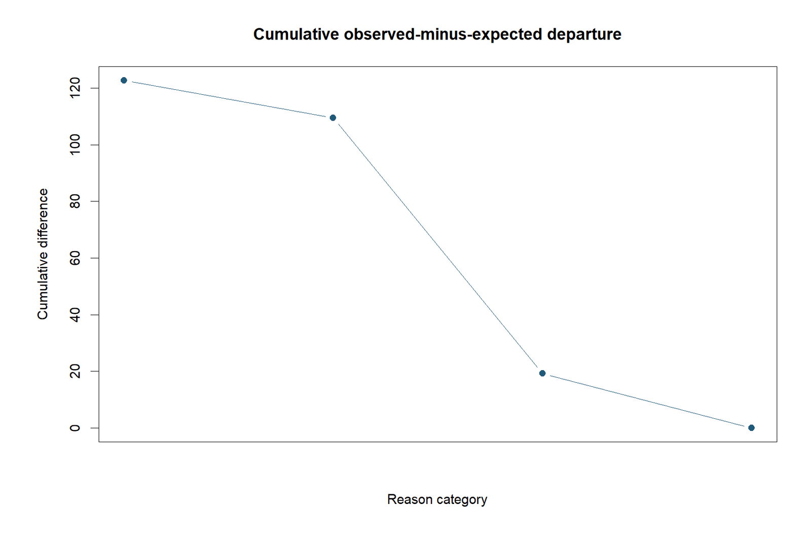
In the displayed category order, cumulative observed-minus-expected differences are +122.75 after course, +109.50 after home, +19.25 after other, and 0 after reputation. The final value must return to zero because total observed and expected counts are equal. For nominal categories, the curve is descriptive and depends on order.
Chi Square Goodness of Fit Test Versus Independence, Homogeneity and Other Tests
One observed categorical variable compared with specified probabilities.
Two categorical variables measured in one population and cross-tabulated.
One categorical outcome compared across separate populations or groups.
Exact inference for a small 2 × 2 contingency table, not a general one-variable multinomial fit test.
| Feature | Goodness of fit | Independence | Homogeneity |
|---|---|---|---|
| Observed variables | One categorical variable | Two categorical variables | One categorical outcome plus population/group source |
| Expected counts | N × specified probability | Row total × column total / N | Row total × column total / N |
| Degrees of freedom | k − 1, minus estimated parameters | (r − 1)(c − 1) | (r − 1)(c − 1) |
| Null hypothesis | Observed distribution matches target | Variables are independent | Populations share the same distribution |
Goodness of Fit Versus Normality Tests
The phrase “goodness of fit” is also used broadly for models and continuous distributions. A Pearson chi square goodness of fit test can assess grouped continuous data against a fitted distribution, but binning choices and estimated parameters affect validity and degrees of freedom. For ordinary normality assessment, dedicated methods and graphical diagnostics are often preferable.
Pearson χ² Versus G²
Pearson χ² uses squared standardized deviations. The likelihood-ratio G² uses 2ΣO log(O/E). Both assess the same null distribution but can differ in small samples. The reported workflow uses Pearson χ² throughout to keep the formula and software outputs consistent.
Chi Square Goodness of Fit Test Calculator: Step-by-Step Workflow
A reliable chi square goodness of fit test calculator should accept category labels, observed counts, and expected proportions. It should verify that the observed counts are nonnegative integers, expected probabilities are nonnegative and sum to 1, and expected counts are adequate.
Calculator Inputs for This Example
Calculator Step 1: Check Totals
The observed total is 285 + 149 + 72 + 143 = 649. The expected proportions total 1.00. A calculator should stop with an error when expected probabilities do not total 1 within a small numerical tolerance.
Calculator Step 2: Generate Expected Counts
Multiply N by each null probability. The calculator should display 162.25 for all four expected counts and should not round these counts before calculating the statistic.
Calculator Step 3: Calculate Contributions
The calculator should show category contributions rather than returning only a global p-value. These contributions reveal that course contributes 92.8663 and other contributes 50.2007.
Calculator Step 4: Calculate χ² and df
Sum the contributions to obtain 146.4329738. With four fixed-probability categories, df = 3.
Calculator Step 5: Calculate the Right-Tail P-Value
The output should use P(Χ²3 ≥ 146.4329738), not a two-tailed normal probability. The result is approximately 1.549 × 10⁻³¹.
Calculator Step 6: Add Effect Size and Interpretation
A complete calculator reports Cohen’s w = 0.475004, observed and expected proportions, signed residuals, and a plain-language conclusion.
Python Chi Square Goodness of Fit Test Charts
The Python workflow produces six figures. Each chart below includes exact values, statistical meaning, and the next reporting step.
Python Chart 1: Observed and Expected Counts
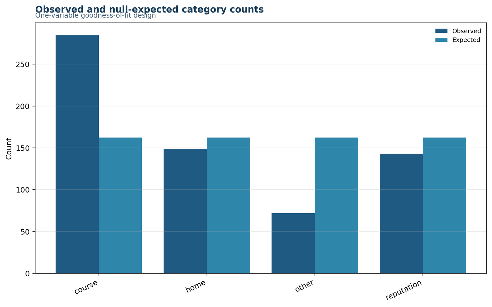
The course bar is far above its equal-share expectation, while the other bar is far below expectation.
Course: 285 observed versus 162.25 expected. Home: 149 versus 162.25. Other: 72 versus 162.25. Reputation: 143 versus 162.25.
The global lack of fit is visible before the statistic is calculated. Course exceeds expectation by 122.75 and other falls short by 90.25.
Report raw counts and expected counts together so readers can see the denominators behind the test.
Python Chart 2: Observed Category Proportions
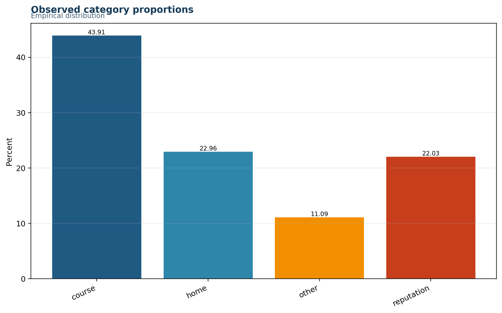
Course is the most common reason and other is the least common.
Course: 43.91%. Home: 22.96%. Other: 11.09%. Reputation: 22.03%. The null reference is 25% for every category.
The substantive distribution is dominated by course, while home and reputation are fairly close to one another and other is much lower.
Percentages make practical magnitude easier to understand than χ² alone.
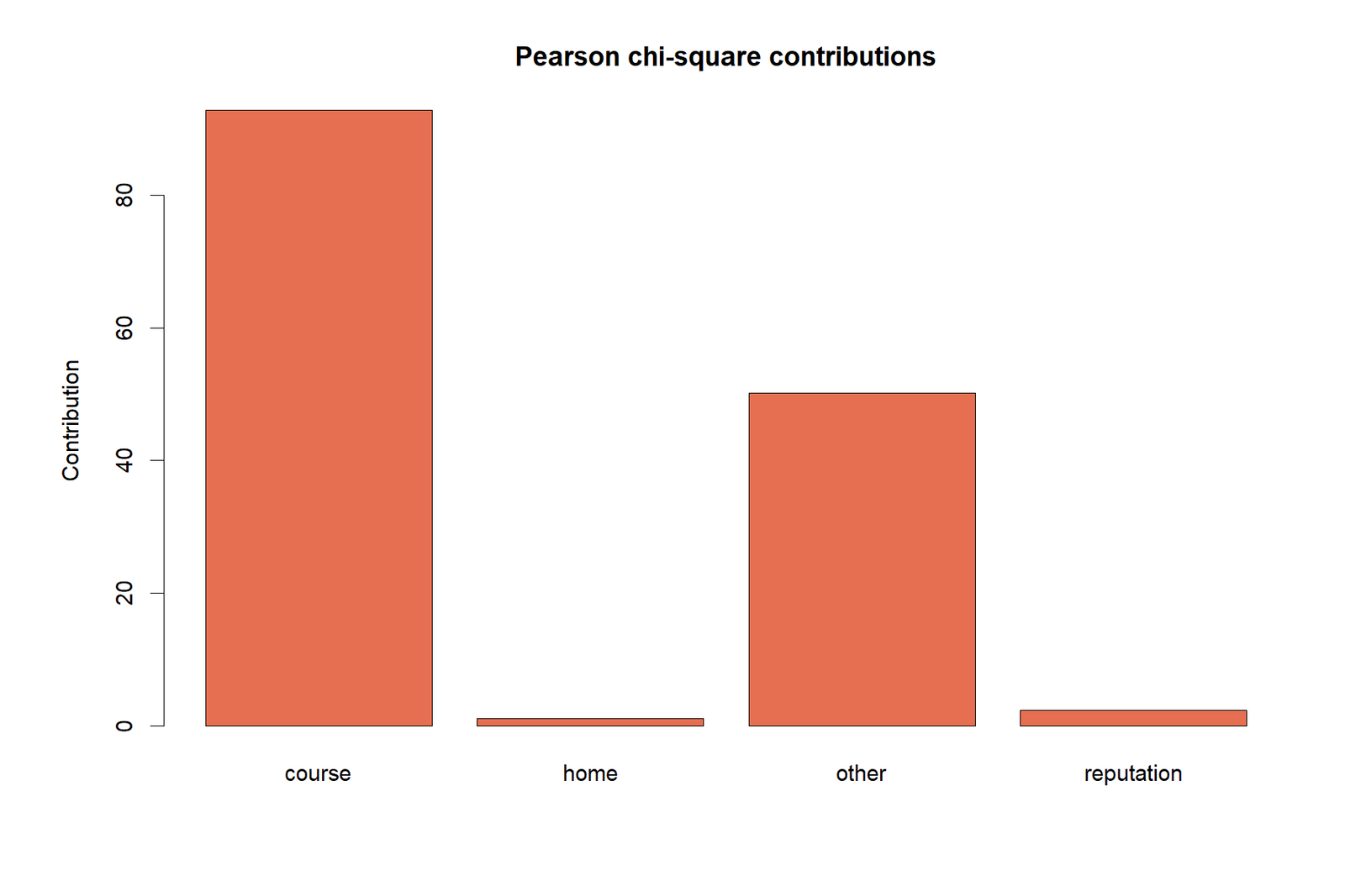
Python Chart 3: Pearson Contributions
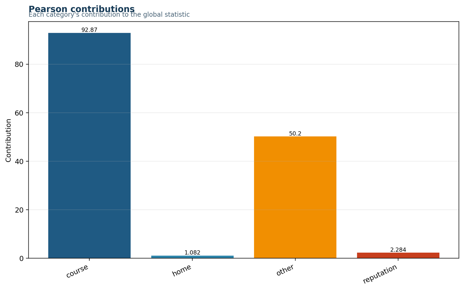
Two bars dominate: course and other.
Course contribution: 92.8663. Other: 50.2007. Home: 1.0820. Reputation: 2.2839.
Course provides 63.42% of χ² and other provides 34.28%; together they explain 97.70% of the statistic.
A significant global chi square goodness of fit test should be decomposed so readers know which categories matter.
Python Chart 4: Signed Contributions
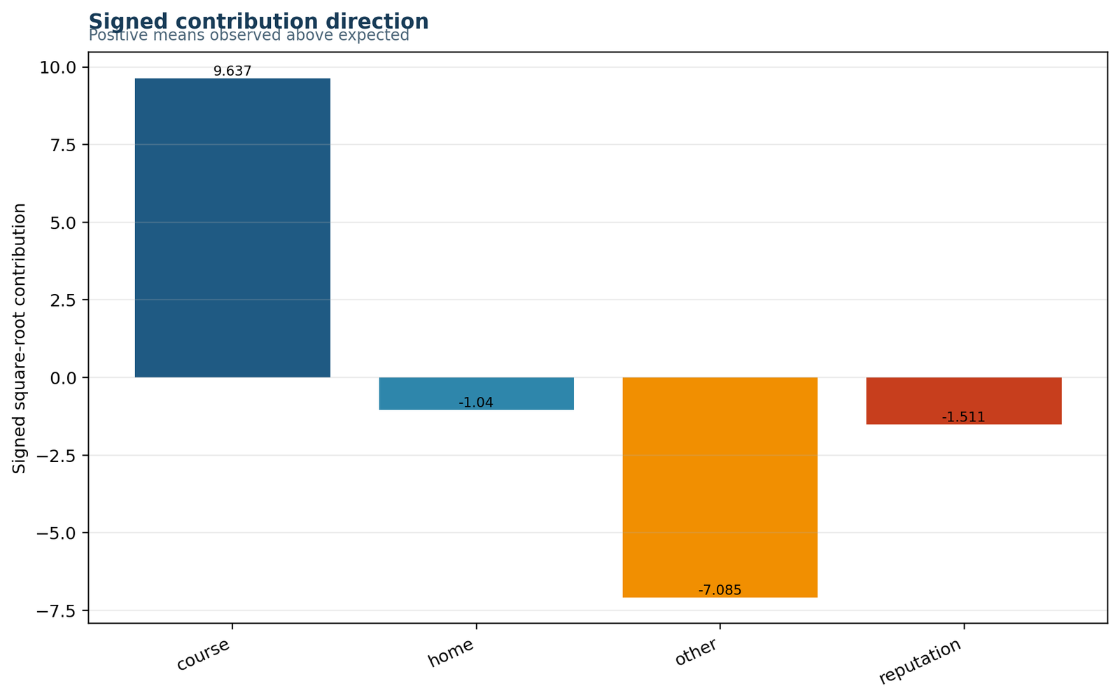
Course is strongly positive, other is strongly negative, and the remaining categories are modestly negative.
Signed roots: course +9.6367, home −1.0402, other −7.0852, reputation −1.5113.
Positive means above expected and negative means below expected. Magnitudes beyond about 2 are substantial diagnostics.
The chart distinguishes overrepresentation from underrepresentation, which the squared statistic cannot do.
Python Chart 5: Null Reference Distribution
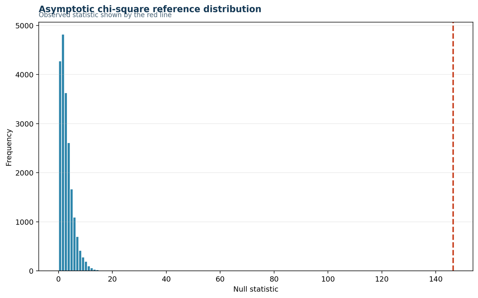
The null distribution is concentrated near zero, while the observed statistic appears far to the right at 146.43.
Observed χ²: 146.432974. df: 3. .05 critical value: 7.8147.
The extreme separation explains the p-value near 1.55 × 10⁻³¹. This is not a borderline threshold result.
The figure makes the right-tailed decision rule intuitive.
Python Chart 6: Result Summary
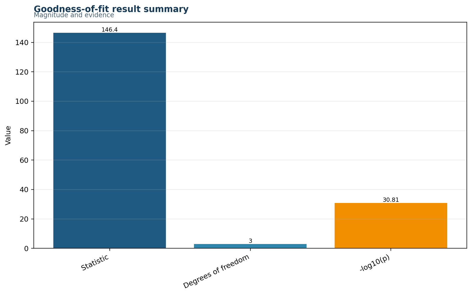
The statistic is large relative to df, and −log10(p) is approximately 30.81.
Statistic: 146.43. Degrees of freedom: 3. −log10(p): 30.81.
The p-value is extremely small, but effect size and category differences remain necessary for substantive interpretation.
Result summaries should not imply that p-value magnitude is an effect size.
R Chi Square Goodness of Fit Test Chart Pairs
The R output is arranged in three balanced pairs. Each figure has its own explanation box so the chart remains useful on desktop and mobile.
Observed and expected counts
Observed counts are 285, 149, 72, and 143; every expected count is 162.25. Course is +122.75 above expected and other is −90.25 below expected.
Contribution by category
Pearson contributions are 92.8663, 1.0820, 50.2007, and 2.2839. Course and other account for 97.70% of χ².
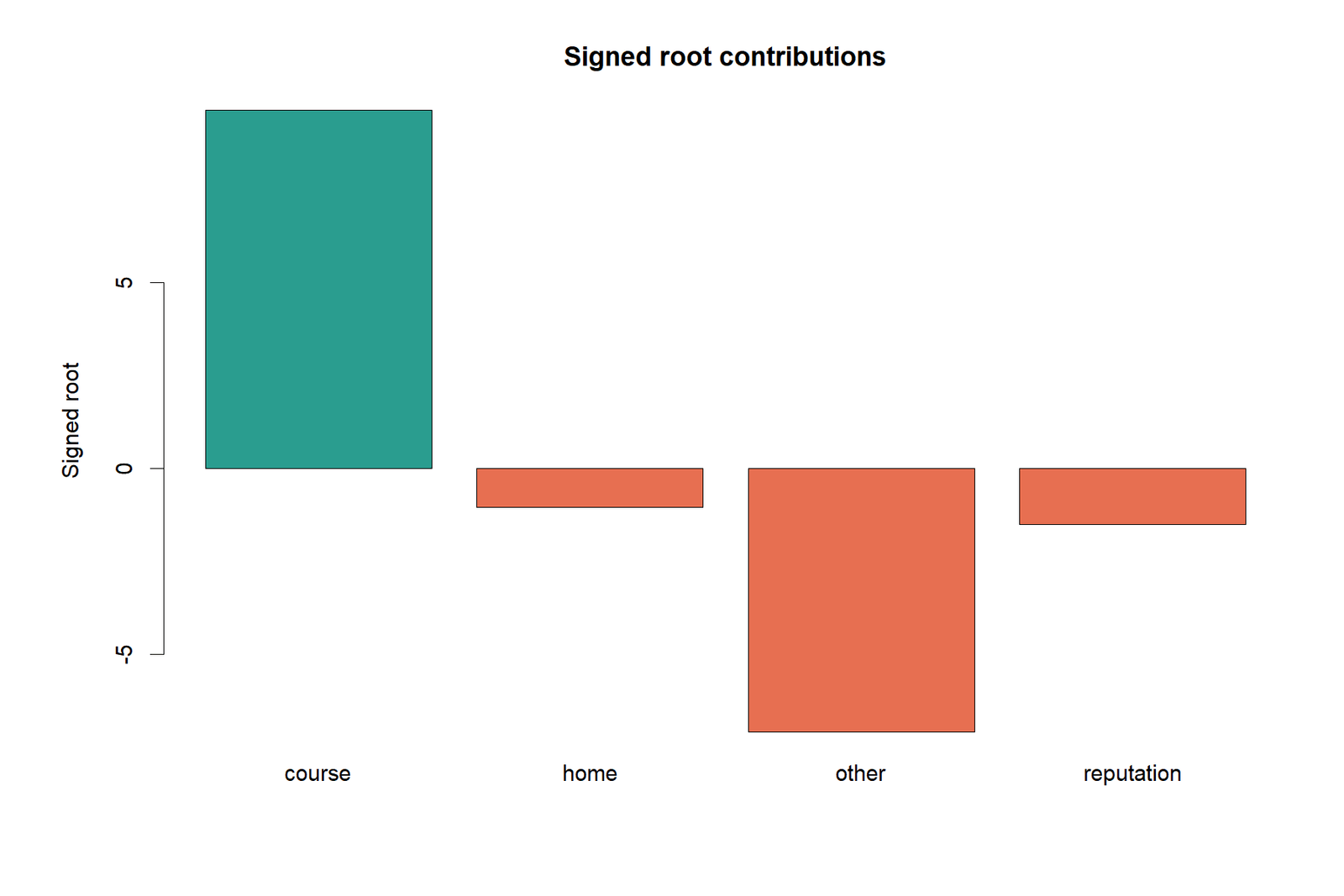
Signed root residuals
The values are +9.6367, −1.0402, −7.0852, and −1.5113. Course and other are the clearly exceptional categories.
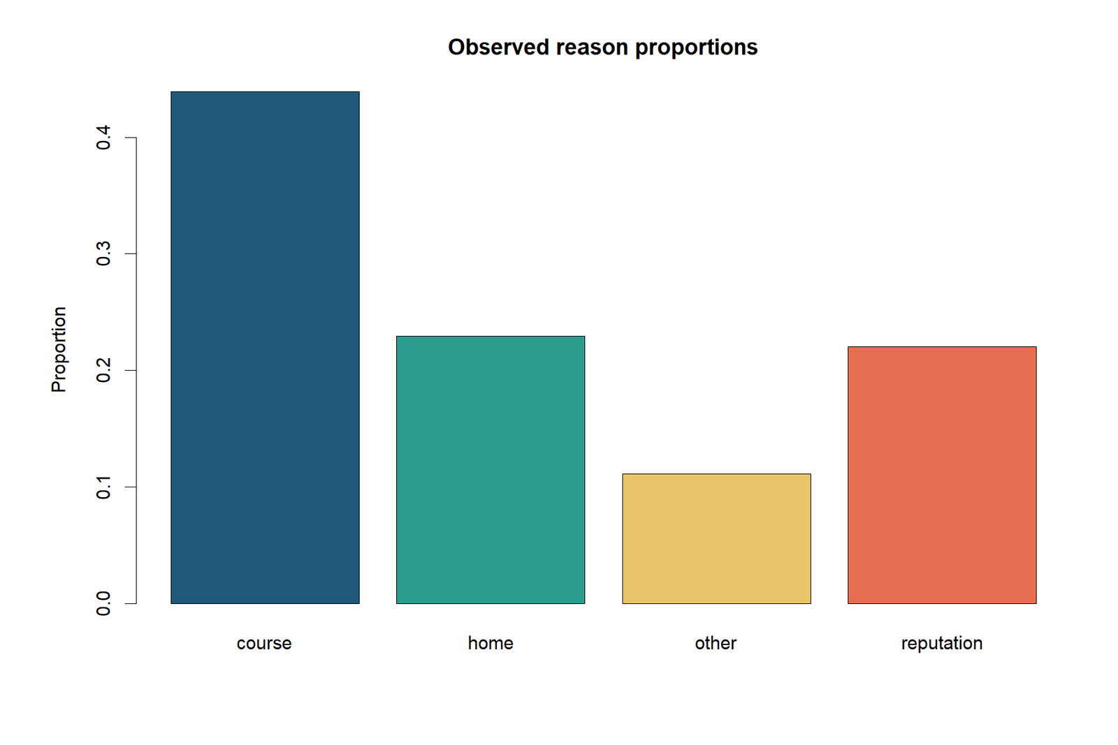
Observed proportions
The empirical shares are 43.91%, 22.96%, 11.09%, and 22.03%, compared with 25% each under H₀.
Result summary
R reproduces χ² = 146.4329738, df = 3, p = 1.549456119 × 10⁻³¹, and maximum |signed root| = 9.6367.
Cumulative departure
Cumulative differences in the displayed order are 122.75, 109.50, 19.25, and 0. The final return to zero is required by equal totals.
Chi Square Goodness of Fit Test in Python, R, SPSS, Excel and Other Software
Python
Use scipy.stats.chisquare with observed counts and expected counts or expected proportions converted to counts. Confirm category order before passing arrays.
- Count the reason categories.
- Set expected proportions to [0.25, 0.25, 0.25, 0.25].
- Calculate expected counts as N × p.
- Request the Pearson statistic and p-value.
- Calculate contributions and Cohen’s w separately.
Target: χ² = 146.4329738, p = 1.549456119 × 10⁻³¹.
R
Use chisq.test(x, p=...). R normalizes the supplied probabilities unless rescale.p=FALSE is used, so explicitly verify the probability vector.
- Create a named count vector.
- Run
chisq.testwith p = rep(.25, 4). - Inspect expected counts and residuals.
- Calculate category contributions.
- Save tables and charts to the R output folders.
SPSS
Use the One-Sample Chi-Square procedure or legacy Nonparametric Tests with expected values specified as equal or custom. SPSS should display observed N, expected N, residuals, χ², df, and asymptotic significance.
- Define the four reason categories.
- Select equal expected values.
- Check that missing categories are handled correctly.
- Do not use CROSSTABS independence output as a substitute.
- Export SAV, SPV, and PDF where available.
Excel
Excel can reproduce the full manual calculation. Use formulas for expected counts, contributions, χ², df, p-value, and effect size.
Expected = Total × Expected proportionContribution = (Observed − Expected)^2 / ExpectedStatistic = SUM(contributions)P-value = CHISQ.DIST.RT(statistic, df)w = SQRT(statistic / total)
TI-84
Many TI-84 models provide a χ² GOF-Test under STAT TESTS. Enter observed counts in one list and expected counts in another, then select the correct degrees of freedom.
- L1: 285, 149, 72, 143
- L2: 162.25, 162.25, 162.25, 162.25
- df: 3
- Read χ² and p from the output.
StatCrunch, Minitab, SAS and Stata
Each package has a one-sample categorical or frequency-table workflow. The essential validation is identical: one observed count vector, one expected probability vector, correct category alignment, df adjustment when parameters are estimated, and right-tail p-value interpretation.
Expandable Chi Square Goodness of Fit Test Code
Python code
import numpy as np
from scipy.stats import chisquare

labels = np.array(["course", "home", "other", "reputation"])
observed = np.array([285, 149, 72, 143], dtype=float)
probabilities = np.repeat(0.25, 4)
expected = observed.sum() * probabilities

result = chisquare(f_obs=observed, f_exp=expected)
contributions = (observed - expected) ** 2 / expected
signed_roots = np.sign(observed - expected) * np.sqrt(contributions)
cohens_w = np.sqrt(result.statistic / observed.sum())

print(result.statistic)  # 146.43297380585514
print(result.pvalue)     # 1.5494561192342533e-31
print(contributions)
print(signed_roots)
print(cohens_w)          # 0.4750038095798172
R code
observed <- c(course=285, home=149, other=72, reputation=143)
expected_p <- c(.25, .25, .25, .25)
fit <- chisq.test(observed, p=expected_p, rescale.p=FALSE)

expected <- fit$expected
contribution <- (observed - expected)^2 / expected
signed_root <- sign(observed - expected) * sqrt(contribution)
cohens_w <- sqrt(unname(fit$statistic) / sum(observed))

fit
contribution
signed_root
cohens_w
SPSS syntax outline
* reason must be coded as four numeric categories before this block.
NPAR TESTS
  /CHISQUARE=reason(1,4)
  /EXPECTED=EQUAL
  /MISSING ANALYSIS.

* Verify expected N = 162.25 in all four categories.
* Verify Chi-Square = 146.432974 and df = 3.
Excel formula layout
A2:A5  Category labels
B2:B5  Observed counts
C2:C5  Expected proportions
D2     =SUM($B$2:$B$5)*C2
E2     =(B2-D2)^2/D2
F2     =SIGN(B2-D2)*SQRT(E2)
E6     =SUM(E2:E5)
E7     =ROWS(A2:A5)-1
E8     =CHISQ.DIST.RT(E6,E7)
E9     =SQRT(E6/SUM(B2:B5))
Advanced Chi Square Goodness of Fit Test Topics
Unequal Expected Proportions
Replace the equal 0.25 vector with the theory-based probabilities. Expected counts remain Npj. The probabilities must be fixed before inspecting the current sample unless the analysis explicitly adjusts degrees of freedom for estimated parameters.
Estimated Parameters and Degrees of Freedom
When fitting a Poisson, normal, or another distribution to grouped data, parameters estimated from the same sample consume degrees of freedom. A common form is df = number of usable categories − 1 − number of estimated parameters. The exact adjustment depends on the model and grouping procedure.
Combining Sparse Categories
Categories should not be combined merely to obtain significance. Combining may be defensible when categories are substantively similar and the rule is chosen without reference to observed departures. Report the original categories, the rationale, and the resulting expected counts.
Exact and Monte Carlo Alternatives
When expected counts are too small for the asymptotic chi-square approximation, an exact multinomial test or Monte Carlo p-value can be used. Software-specific implementation details should be documented, including the number of simulations and random seed for reproducibility.
Structural Zeros
A structural zero is a category that cannot occur by design. It should not be treated as an ordinary zero-count category with positive expected probability. The null model and degrees of freedom must reflect the restricted sample space.
Power and Sample Size
Power depends on alpha, degrees of freedom, sample size, and the alternative effect size w. A prospective power analysis requires a meaningful expected distribution and a plausible alternative distribution. Using an arbitrary w without substantive justification can produce a misleading sample-size target.
Confidence Intervals for Category Proportions
The global chi square goodness of fit test does not return confidence intervals. Binomial or multinomial intervals can be added for each observed proportion. Simultaneous intervals are preferable when the goal is to make several category-specific statements while controlling familywise error.
Survey Weights and Complex Samples
Ordinary Pearson calculations assume unweighted independent observations. Survey weights, strata, and clusters require design-based procedures. Treating weighted counts as if they were raw counts can severely understate uncertainty.
Repeated or Clustered Categories
If multiple responses come from the same person or students are nested in schools, the independence assumption can fail. Generalized estimating equations, mixed models, or survey-adjusted tests may be more appropriate than a basic chi square goodness of fit test.
Sensitivity to the Null Model
The same observed counts can produce a different conclusion under a different expected distribution. A scientifically defensible report explains why the selected null probabilities represent the research claim. Testing multiple target distributions after viewing results creates a model-selection problem and should be disclosed.
APA Reporting for a Chi Square Goodness of Fit Test
Concise Result
A chi square goodness of fit test showed that school-choice reasons were not equally distributed, χ²(3, N = 649) = 146.43, p < .001, Cohen’s w = .475.
Expanded Result
The observed distribution of school-choice reasons differed significantly from an equal four-category distribution, χ²(3, N = 649) = 146.43, p < .001, w = .475. Course was more frequent than expected (285 observed, 162.25 expected), whereas other was less frequent than expected (72 observed, 162.25 expected).
Copy-Ready Templates
Significant result template
Reject H₀
A chi square goodness of fit test compared observed variable with expected distribution.
The distributions differed, χ²(df, N = N) = statistic, p p-value, w = effect size.
Category was above expectation, whereas category was below expectation.
Nonsignificant result template
Retain H₀
A chi square goodness of fit test evaluated whether observed categories matched expected probabilities.
The evidence did not show a departure, χ²(df, N = N) = statistic, p = p-value, w = effect size.
Reporting Checklist
- Name the Pearson chi square goodness of fit test.
- Identify the observed variable and categories.
- State the expected probabilities.
- Report χ², df, N, and p.
- Report Cohen’s w or another justified effect size.
- Describe the main overrepresented and underrepresented categories.
- State any multiple-comparison method used for follow-up tests.
Common Chi Square Goodness of Fit Test Mistakes
Design Mistakes
- Using goodness of fit when two observed variables are present.
- Choosing equal probabilities without a substantive reason.
- Treating repeated observations as independent.
- Using overlapping categories.
- Ignoring unobserved or missing categories that belong in the target distribution.
Calculation and Reporting Mistakes
- Entering percentages instead of counts.
- Rounding expected counts before calculating contributions.
- Using df = k rather than k − 1.
- Reading a left-tail or two-tailed probability.
- Reporting p = .000.
- Interpreting χ² as effect size.
- Failing to explain which categories drive significance.
Mistake: Expected Counts Equal Observed Totals by Category
Expected counts come from the null probabilities, not from averaging observed and expected columns or from using each observed percentage as its own expectation. In the current chi square goodness of fit test, all expected counts are 162.25 because the null probabilities are all .25.
Mistake: Calling the Test Two-Tailed
Because χ² is a sum of nonnegative contributions, evidence against H₀ appears in the upper tail. Direction is recovered through residuals, not through a negative chi-square statistic or a two-tailed p-value.
Mistake: Concluding Every Category Differs
The omnibus result says at least one probability differs. Home and reputation make small contributions. Course and other drive the result. Formal category-specific conclusions need follow-up methods and multiplicity control.
Chi Square Goodness of Fit Test Practice Problems
Practice 1: Equal Four-Category Distribution
A sample contains observed counts 44, 56, 50, and 50. Test equal proportions at α = .05.
Practice 2: Unequal Expected Distribution
Observed counts are 120, 90, 60, and 30. The expected proportions are .40, .30, .20, and .10. Perform the test.
Practice 3: Identify the Correct Chi-Square Test
A researcher records sex and preferred learning mode for 500 students. Is this a chi square goodness of fit test?
Practice 4: Degrees of Freedom
A goodness-of-fit test has six categories and fixed expected probabilities. What is df?
Practice 5: Interpret a Residual
A category has observed count 90 and expected count 50. What does the sign of its residual mean?
Chi Square Goodness of Fit Test Study Notes
Always right-tailed
The chi square goodness of fit test is right-tailed because the statistic is a sum of nonnegative squared contributions.
Counts first
The chi square goodness of fit test formula uses observed and expected counts; percentages support interpretation but do not replace counts.
Null probabilities
A chi square goodness of fit test requires expected probabilities that are explicit, defensible, and sum to 1.
Expected values
Expected counts for a chi square goodness of fit test equal sample size multiplied by each null probability.
Degrees of freedom
For fixed probabilities, the chi square goodness of fit test usually has k − 1 degrees of freedom.
Effect size
Cohen’s w adds practical magnitude to a chi square goodness of fit test result.
Residual direction
Signed residuals show whether each category in a chi square goodness of fit test is above or below expectation.
Large samples
A chi square goodness of fit test can detect small departures when N is large, so effect size remains essential.
Small expected counts
When expected counts are sparse, an exact or simulation-based alternative to the asymptotic chi square goodness of fit test may be needed.
One variable
A chi square goodness of fit test analyzes one categorical variable, not an association between two observed variables.
Equal distribution
An equal-proportions chi square goodness of fit test is appropriate only when equality is the actual null claim.
Unequal distribution
A chi square goodness of fit test can evaluate any valid probability vector, not only equal proportions.
Omnibus conclusion
A significant chi square goodness of fit test says the full distribution differs but does not prove that every category differs.
Category order
Reordering nominal categories does not change the chi square goodness of fit test statistic.
Missing data
A chi square goodness of fit test should use a transparent rule for missing and invalid category values.
Independent rows
The chi square goodness of fit test assumes each row contributes one independent categorical observation.
Critical values
The chi square goodness of fit test can be decided with a right-tail p-value or the equivalent chi-square critical value.
APA style
An APA chi square goodness of fit test report includes χ², df, N, p, effect size, and the main category departures.
No p equals zero
A chi square goodness of fit test with a tiny probability should be reported as p < .001 rather than p = .000.
No causality
A chi square goodness of fit test identifies distributional mismatch but does not explain its cause.
Pre-specification
Expected probabilities for a chi square goodness of fit test should not be selected after searching for the most significant result.
Weighted data
A basic chi square goodness of fit test is not automatically valid for complex survey weights and clustered designs.
Software agreement
Python, R, SPSS, and Excel should reproduce the same chi square goodness of fit test when inputs and conventions match.
Parameter estimation
A grouped-distribution chi square goodness of fit test may require a degrees-of-freedom adjustment when parameters are estimated.
Interpretation order
Interpret a chi square goodness of fit test by reading the null model, observed proportions, effect size, residuals, and p-value together.
Chi Square Goodness of Fit Test Downloads
Use the verified reports and worked workbook to reproduce the analysis and compare software output.
Frequently Asked Questions
What is a chi square goodness of fit test?
A chi square goodness of fit test compares one observed categorical frequency distribution with a specified set of expected population proportions.
When should I use a chi square goodness of fit test?
Use it when one categorical variable is measured, observations are independent, expected probabilities are specified, and expected counts are adequate.
What is the null hypothesis?
The null hypothesis states that the population category probabilities equal the specified expected probabilities.
What is the alternative hypothesis?
At least one population category probability differs from its null value.
What is the formula?
The statistic is χ² = Σ(O − E)²/E, summed across all categories.
How are expected counts calculated?
Multiply the total sample size by each expected probability.
What are the degrees of freedom?
With k categories and no estimated parameters, df = k − 1.
Why is the test right-tailed?
Only large nonnegative chi-square values indicate poor fit because all category contributions are squared.
Can expected counts be decimals?
Yes. Expected counts are theoretical values and do not need to be integers.
Can the expected proportions be unequal?
Yes. Any valid theory-based probabilities may be used as long as they sum to 1.
What is the difference from a test of independence?
Goodness of fit analyzes one categorical variable against a target distribution; independence analyzes the association between two observed categorical variables.
What does a significant result mean?
The observed frequency vector is inconsistent with the specified expected vector, assuming the model and sampling conditions are valid.
Does significance mean every category differs?
No. The test is omnibus. Contributions and multiplicity-adjusted follow-ups identify the main departures.
How do I interpret residuals?
Positive residuals indicate observed counts above expectation; negative residuals indicate counts below expectation.
What effect size should I report?
Cohen’s w is a common overall effect size for a one-sample categorical goodness-of-fit analysis.
What if expected counts are below 5?
Consider combining categories only when substantively defensible, or use an exact or Monte Carlo multinomial procedure.
How do I report a tiny p-value?
Report p < .001 in ordinary prose rather than p = .000. Technical output may preserve the exact scientific-notation value.
Can I run the test in Excel?
Yes. Excel can calculate expected counts, contributions, χ², df, the right-tail p-value, and Cohen’s w.
Can I run the test in Python?
Yes. SciPy’s chisquare function reproduces the Pearson result when observed and expected arrays are aligned.
Can I run the test in R?
Yes. Use chisq.test with a count vector and the expected probability vector.
Can SPSS perform the test?
Yes. Use the one-sample chi-square procedure with equal or user-specified expected values.
Is the test parametric?
It is commonly called nonparametric because it analyzes category counts without normality assumptions, but it still has important design and expected-count conditions.
What is the result in this worked example?
The verified result is χ²(3, N = 649) = 146.43, p < .001, w = .475.
Which categories drive the result?
Course is strongly above expectation and other is strongly below expectation; together they account for 97.70% of χ².
Conclusion
The chi square goodness of fit test is the correct one-variable procedure when observed categorical counts are compared with a fully specified probability distribution. In the verified 649-student example, the four school-choice reasons do not follow an equal distribution, χ²(3) = 146.4329738, p = 1.549456119 × 10⁻³¹. Course is substantially overrepresented, other is substantially underrepresented, and Cohen’s w = 0.475 indicates a large overall discrepancy.
A strong report combines the global chi square goodness of fit test with observed and expected counts, category proportions, signed residuals, contribution shares, assumptions, effect size, and a transparent statement of the expected distribution. The supplied Python, R, and Excel downloads reproduce the complete calculation.

