Stepwise Regression: AIC Selection, Formula, Diagnostics, Python, R, SPSS and Excel
Stepwise Regression is presented as a complete model-selection workflow rather than a shortcut to significance. This worked guide follows every saved AIC state from an intercept-only model to a five-predictor equation, compares the selected and full candidate fits, interprets post-selection coefficients, audits residual and influence evidence, and separates Python AIC selection from R, SPSS and Excel alternatives.
Stepwise Regression Model Overview
Stepwise Regression is an algorithmic procedure for choosing a linear-model formula from a prespecified candidate set. The method answers a limited question: which sequence of allowed one-term additions and removals produces the best value of the declared criterion from the declared starting model? The answer is conditional on the sample, candidate pool, direction, likelihood convention and stopping rule.
Use Stepwise Regression for transparent exploratory screening when many plausible predictors compete for a parsimonious equation and the complete path will be preserved. It should not be used to manufacture a confirmatory model, to search repeatedly until every p-value is small, or to replace subject-matter decisions about outcome timing, coding, interactions and confounding.
The verified Python procedure begins with an intercept-only model and considers twelve candidates: G1, G2, absences, studytime, failures, age, Medu, Fedu, traveltime, famrel, freetime and goout. At each state it evaluates every valid one-term addition and removal, accepts the candidate with the smallest AIC when AIC decreases, and stops when no legal move improves the criterion.
The final selected equation contains G2, G1, failures, absences and studytime. G2 enters first and supplies nearly all of the initial predictive gain. Studytime enters last with an AIC decrease of only 0.465715, illustrating why selected membership and conventional p-value thresholds need not agree.
A selected coefficient retains the usual conditional linear-regression units but inherits selection uncertainty. The G2 slope of 0.885709 means that, within the adaptively selected five-term equation, a one-point G2 difference is associated with approximately 0.885709 points in fitted G3 when G1, failures, absences and studytime are fixed. It is not a causal effect and its ordinary interval treats the final formula as if it had been prespecified.
Stepwise Regression differs from best-subset selection, Lasso Regression, Ridge Regression and Elastic Net Regression. A greedy path does not examine every subset. Penalized methods optimize a continuous objective rather than repeatedly refitting discrete candidate formulas. A theory-defined Ordinary Least Squares Regression model remains the clearest benchmark when the formula can be specified before seeing the outcome evidence.
The advantages are a compact path, explicit complexity penalty and a reproducible final formula. The limitations are path dependence, candidate dependence, instability under resampling and optimistic ordinary inference. In the worked analysis, all candidate models use the same 649 complete rows, making their AIC values directly comparable.
Quick Answer
The verified Stepwise Regression path starts at AIC 3364.926948 and accepts five additions. No accepted removal appears in the saved path.
What the output supports
- G2 provides the dominant first criterion improvement.
- G1, failures and absences provide smaller additional AIC decreases.
- Studytime is retained because it lowers AIC, despite p = 0.118199.
- The selected model has lower AIC and BIC than the full candidate model.
What the output does not prove
- The five selected variables are not the only scientifically relevant predictors.
- The ordinary p-values are not adjusted for searching.
- The fitted RMSE is not performance on an untouched validation sample.
- The entry order is not a causal or temporal priority ranking.
Table of Contents
- Model Overview
- Quick Answer
- Why Stepwise Regression Is Needed
- How Stepwise Regression Works
- Variables and Coding
- Verified Results
- Python Chart Stories
- R Chart Pairs
- Coefficient Interpretation
- Predictions and Meaning
- Assumptions and Diagnostics
- Python, R, SPSS and Excel
- Code and Formulas
- Advanced Topics
- APA-Style Reporting
- Publication Checklist
- Downloads
- Related Guides
- Frequently Asked Questions
- Conclusion
Why This Analysis Needs Stepwise Regression
The supplied analysis begins with twelve plausible main-effect predictors but seeks a smaller explanatory and prediction equation. Fitting every candidate automatically would preserve slightly more in-sample fit but would require seven additional slopes. A transparent criterion-based screen can show whether those extra terms provide enough likelihood improvement to justify their complexity.
Stepwise Regression supplies that audit only when the candidate family and search rule are fixed in advance. It records which term is considered at each accepted state and quantifies the AIC change. This is more informative than publishing only the final five-variable formula.
The first G2 move is overwhelming, whereas the final studytime move is weak. Treating both as equally stable because both appear in the endpoint would hide the most important selection evidence.
How Stepwise Regression Works
Criterion and Search State
For each fitted candidate M, AIC combines maximized likelihood with a penalty for the number of estimated parameters. Lower values are preferred among models fitted to the same outcome observations under the same likelihood convention.
Both-Direction Search
From the current formula, the algorithm fits every valid one-term addition and every valid one-term removal. The candidate with the lowest AIC becomes the next state only when it improves on the current AIC.
Verified Path
The path is intercept only → G2 → G2 + G1 → G2 + G1 + failures → G2 + G1 + failures + absences → G2 + G1 + failures + absences + studytime. No term is removed after entering in the saved sequence.
AIC and Ordinary p-Values
AIC evaluates penalized likelihood for the whole model. A coefficient p-value tests one slope under a formula treated as fixed. The two rules need not agree. Studytime lowers AIC slightly even though its conventional endpoint interval crosses zero.
Stopping Rule
The final model is reached because no remaining one-term addition or removal has a lower AIC under the implemented search. That stopping result is conditional on the twelve supplied main effects and the intercept-only start.
Variables Used, Coding and Standardization
The candidate definitions and complete-case rule remain fixed throughout the search.
| Role | Variable | Coding or unit | Selection status |
|---|---|---|---|
| Outcome | G3 | Final grade on the original score scale | Dependent variable in every candidate model |
| Prior achievement | G2 | Second-period grade points | Selected first |
| Prior achievement | G1 | First-period grade points | Selected second |
| Academic history | failures | Previous class-failure count | Selected third |
| Attendance | absences | School absence count | Selected fourth |
| Study exposure | studytime | Ordered weekly study-time code | Selected fifth |
| Demographic | age | Age in years | Eligible but not selected |
| Family education | Medu | Mother’s education code | Eligible but not selected |
| Family education | Fedu | Father’s education code | Eligible but not selected |
| Travel | traveltime | Travel-time category code | Eligible but not selected |
| Family relationship | famrel | Family-relationship quality code | Eligible but not selected |
| Free time | freetime | Free-time category code | Eligible but not selected |
| Social activity | goout | Going-out category code | Eligible but not selected |
The ordered codes are treated as linear numeric terms in the supplied search. Replacing them with indicator variables would change the candidate scope, parameter counts and AIC path.
Verified Stepwise Regression Results
Complete AIC Selection Path
| State | Accepted move | Current terms | AIC | AIC change | Adjusted R-squared |
|---|---|---|---|---|---|
| 0 | Start | Intercept only | 3364.926948 | — | 0.000000 |
| 1 | Add G2 | G2 | 2162.270813 | −1202.656135 | 0.843489 |
| 2 | Add G1 | G2 + G1 | 2147.309621 | −14.961192 | 0.847290 |
| 3 | Add failures | G2 + G1 + failures | 2143.912048 | −3.397573 | 0.848320 |
| 4 | Add absences | G2 + G1 + failures + absences | 2141.719377 | −2.192671 | 0.849063 |
| 5 | Add studytime | G2 + G1 + failures + absences + studytime | 2141.253662 | −0.465715 | 0.849401 |
The first move dominates the path. The last three improvements are much smaller, and the studytime decrease below one identifies a particularly weak endpoint distinction.
Selected versus Full Candidate Model
| Model | Slopes | R-squared | Adjusted R-squared | AIC | BIC | RMSE |
|---|---|---|---|---|---|---|
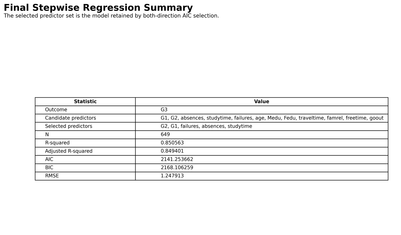
| Selected model | 5 | 0.850563 | 0.849401 | 2141.253662 | 2168.106259 | 1.247913 |
| Full candidate model | 12 | 0.851718 | 0.848921 | 2150.218767 | 2208.399392 | 1.243082 |
The full model improves fitted R-squared by about 0.001155 and lowers RMSE by about 0.004831. The selected model uses seven fewer slopes and has lower AIC and BIC.
Selected Coefficient Evidence
| Term | B | SE | t | Conventional p | Conventional 95% CI |
|---|---|---|---|---|---|
| Intercept | −0.155190 | 0.258626 | −0.6001 | 0.5487 | [−0.6630, 0.3527] |
| G2 | 0.885709 | 0.033927 | 26.1066 | 5.438 × 10−103 | [0.8191, 0.9523] |
| G1 | 0.139457 | 0.036227 | 3.8495 | 0.000130 | [0.0683, 0.2106] |
| failures | −0.218290 | 0.090861 | −2.4025 | 0.0166 | [−0.3967, −0.0399] |
| absences | 0.023367 | 0.010794 | 2.1648 | 0.0308 | [0.0022, 0.0446] |
| studytime | 0.096699 | 0.061810 | 1.5645 | 0.1182 | [−0.0247, 0.2181] |
The endpoint ordinary tests are descriptive because the same outcomes determined the formula. Four selected slopes have conventional p-values below 0.05, while studytime remains because of the AIC rule.
Download the Stepwise Regression Files
The same verified links appear again in the Downloads section.
Python Charts and Exact-Value Explanations
The Python section uses six unique chart stories in the attached template format. Additional diagnostic and summary assets remain available in Downloads.
Python Chart 1: AIC Selection Path
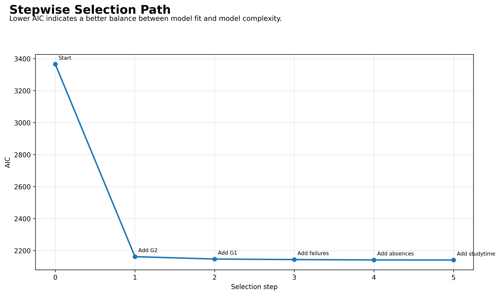
The first G2 addition produces an enormous drop, followed by progressively smaller improvements.
AIC moves from 3364.926948 to 2162.270813, then ends at 2141.253662 after five additions.
The endpoint is generated by a greedy criterion path. Later membership is less strongly separated than the first G2 move.
Publishing every state reveals the relative evidence for each accepted move instead of treating all five terms as equally secure.
Python Chart 2: Selected versus Full Information Criteria
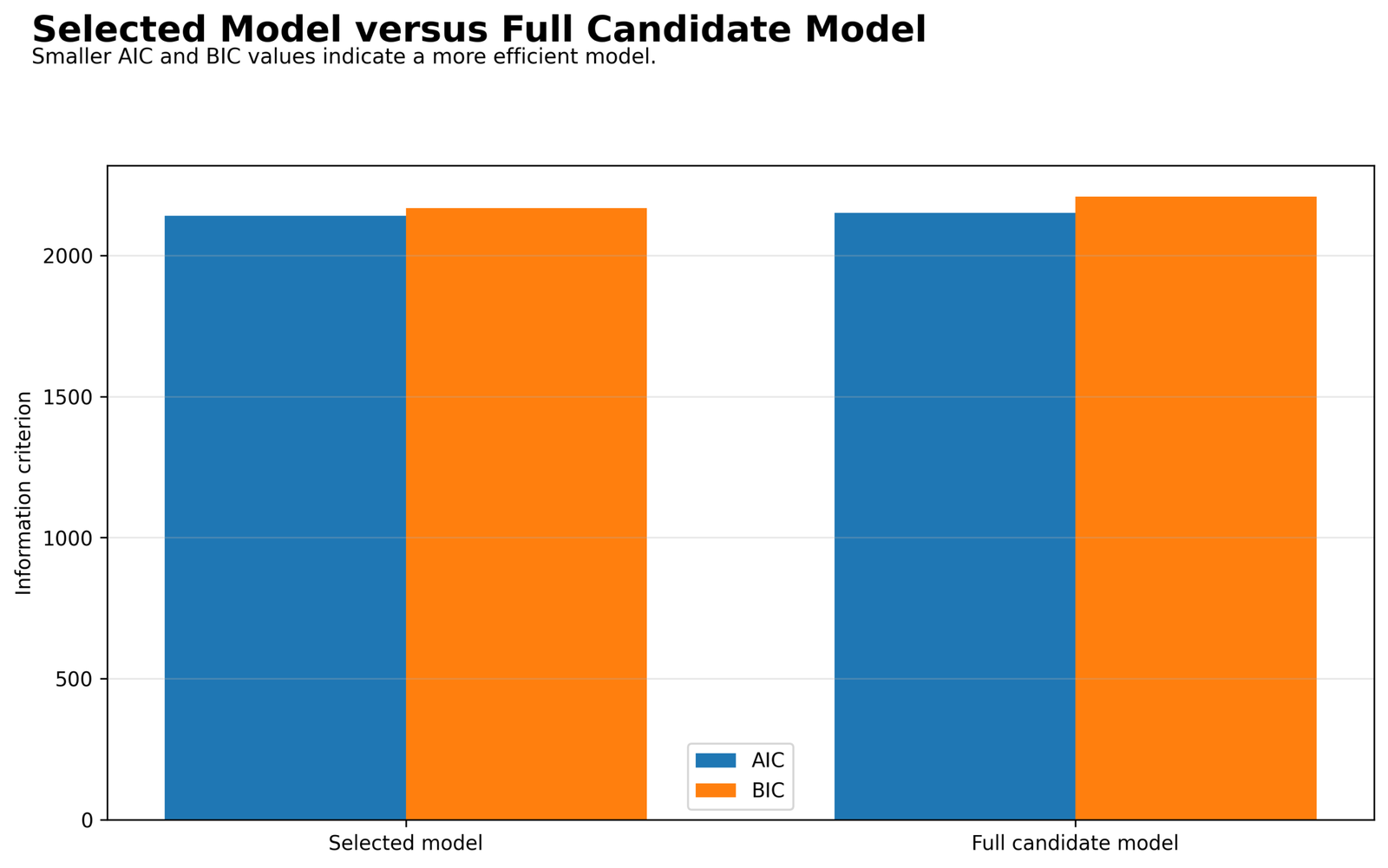
The selected model has lower AIC and BIC despite using fewer terms and having slightly worse fitted RMSE.
Selected AIC/BIC = 2141.253662/2168.106259; full AIC/BIC = 2150.218767/2208.399392.
Information criteria reward the selected model’s parsimony. They do not say its fitted predictions are closer for every observation.
The chart prevents the incorrect statement that the selected model has the lowest value of every fit metric.
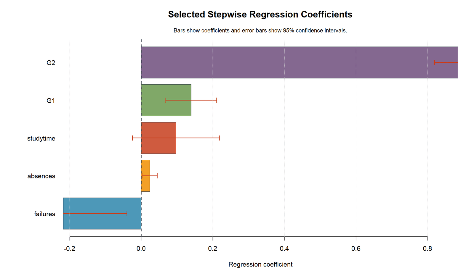
Python Chart 3: Selected Coefficients with Intervals
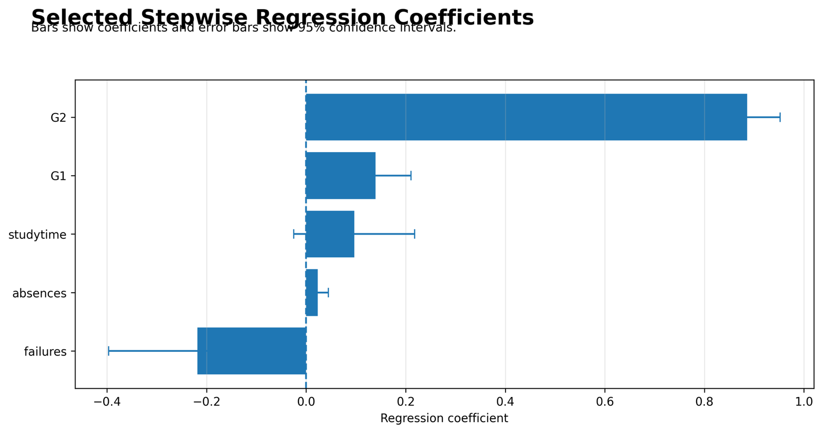
G2 dominates the coefficient scale, failures is negative, and studytime has an interval crossing zero.
G2 = 0.885709; G1 = 0.139457; failures = −0.218290; absences = 0.023367; studytime = 0.096699.
The intervals condition on the selected formula and do not account for the candidate search that produced it.
Direction, magnitude and uncertainty remain more informative than labeling selected membership alone.
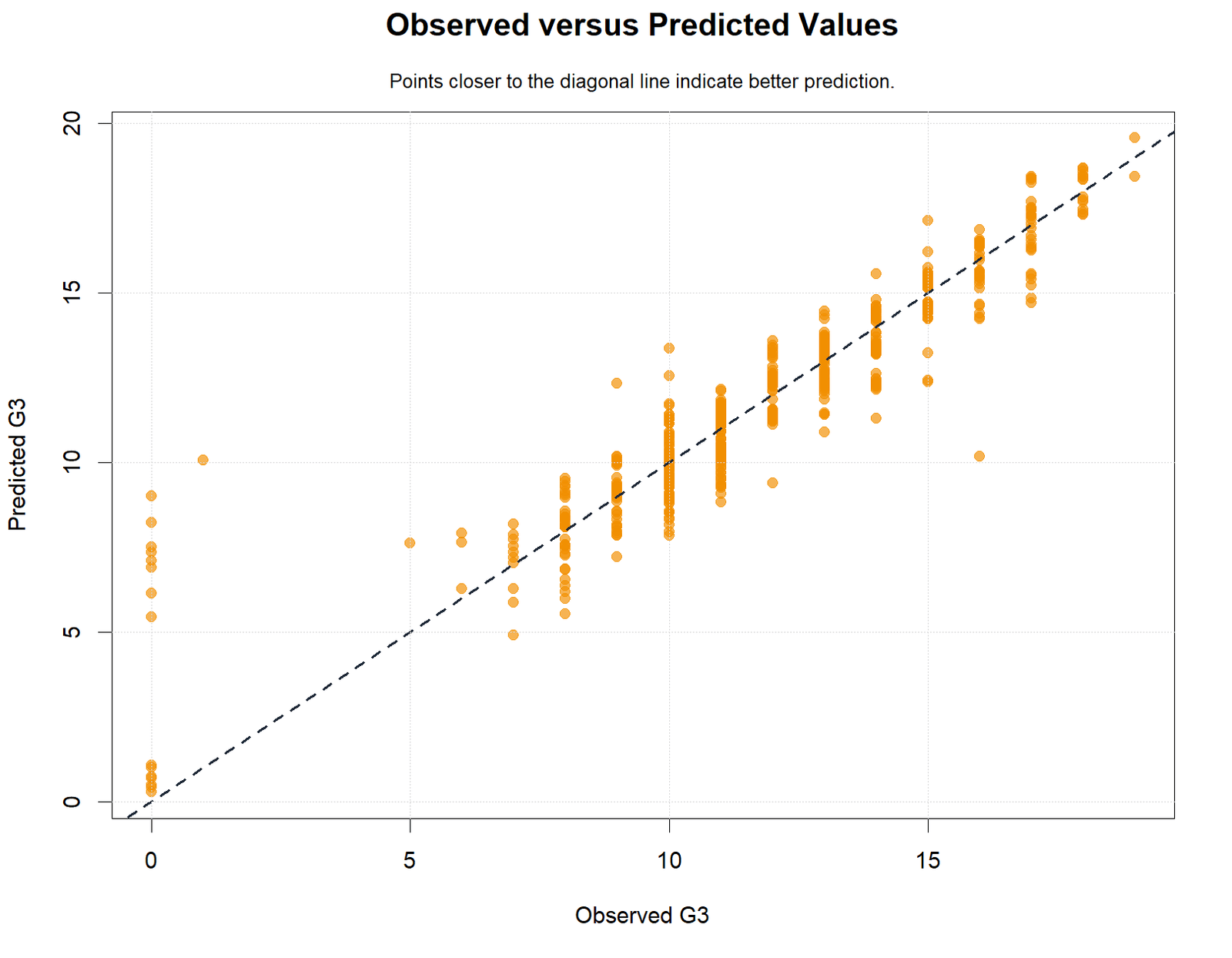
Python Chart 4: Observed versus Predicted G3
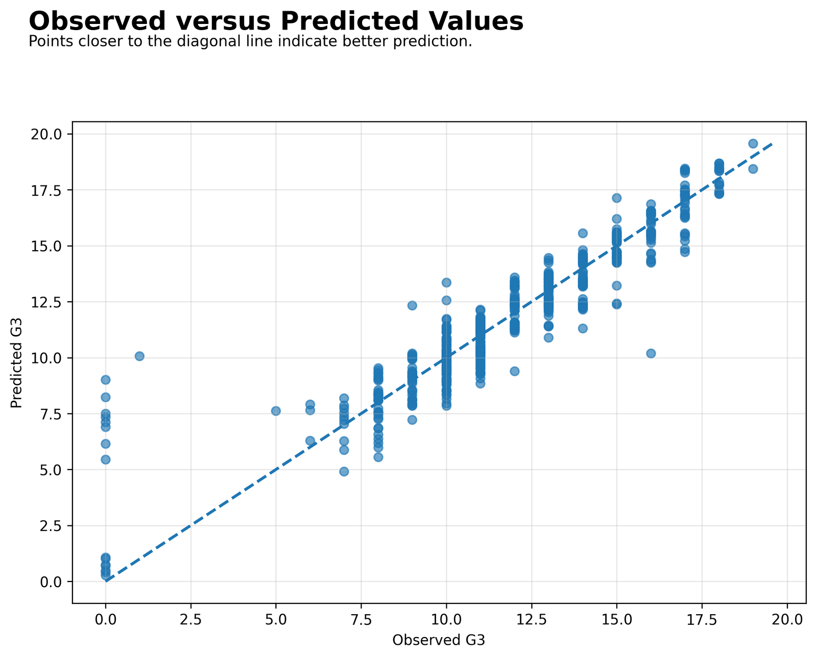
Most observations follow the diagonal in the central grade range, while some boundary outcomes show larger errors.
Selected R-squared = 0.850563, fitted RMSE = 1.247913 and MAE = 0.782996.
The graph describes the same data used to choose and estimate the model. It is not an external prediction assessment.
Strong fitted alignment can coexist with selection optimism and poor transport to a new cohort.
Python Chart 5: Residuals versus Fitted Values
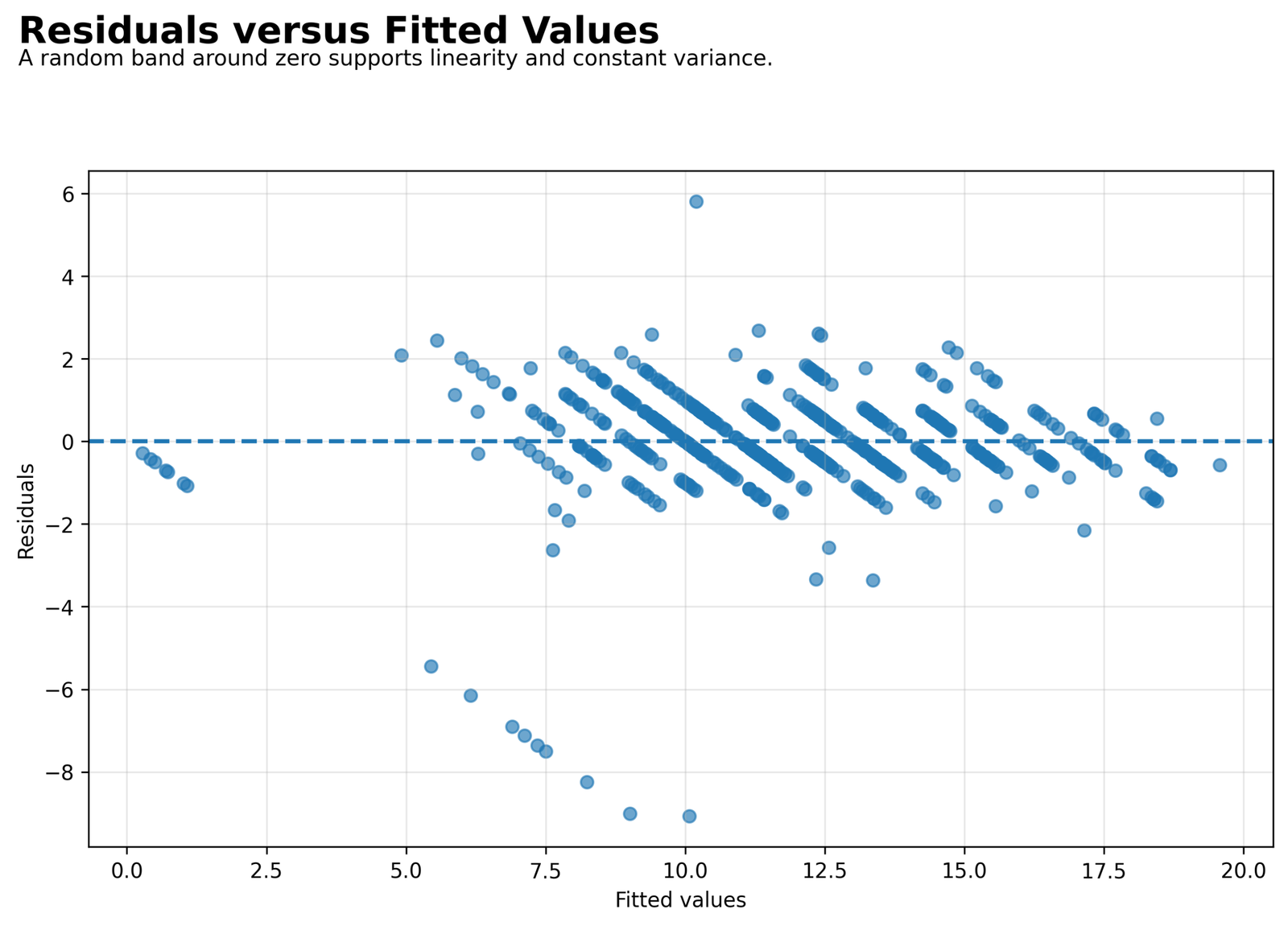
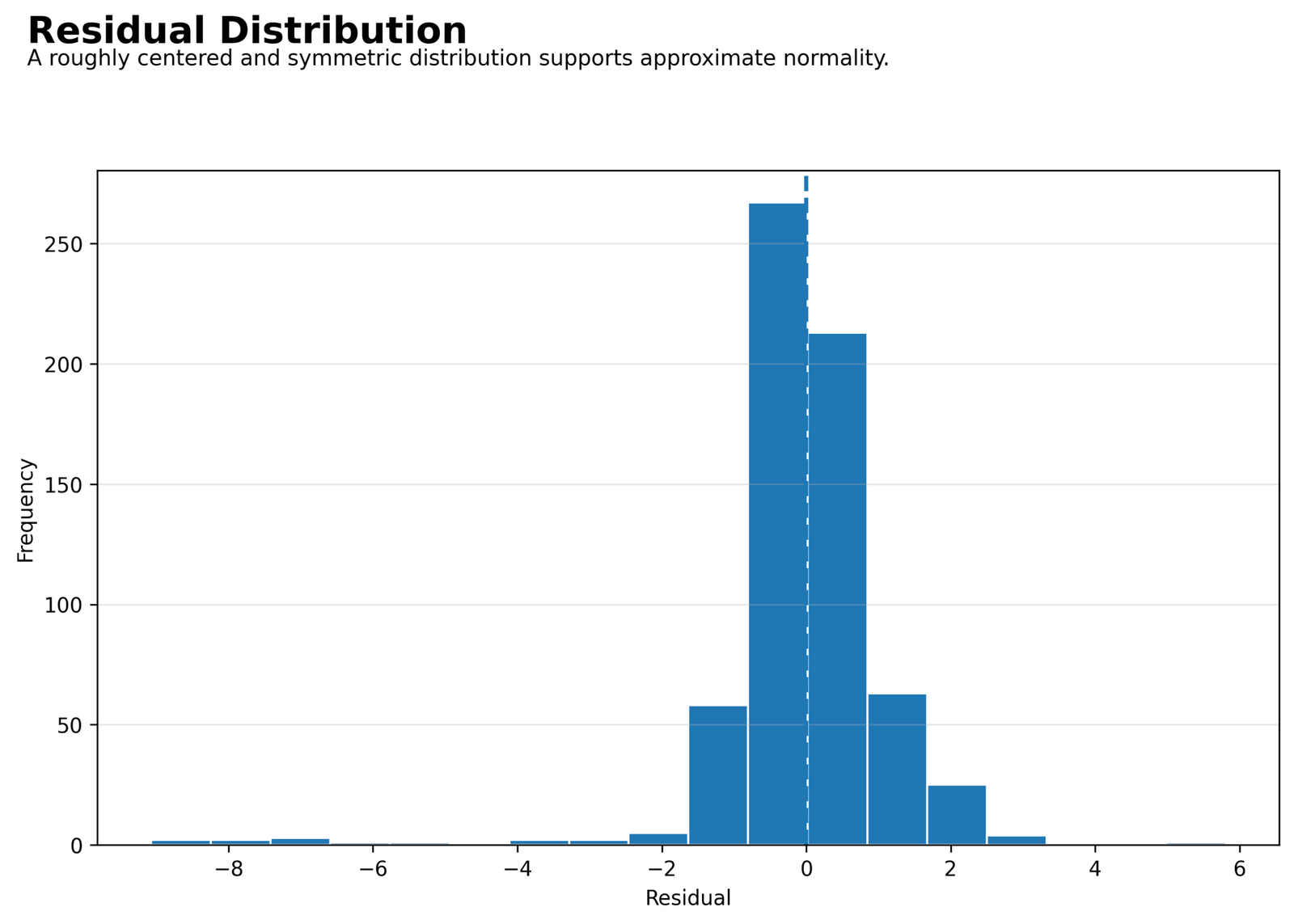
Residuals are broadly centered, integer grades create visible bands, and some large negative errors remain.
Durbin-Watson = 1.857347. Fitted RMSE = 1.247913 for all 649 selected-model residuals.
AIC selection does not guarantee linearity, constant variance, independent errors or correct coding.
Residual misspecification can invalidate the candidate family even when the search path is calculated correctly.
Python Chart 6: Leverage versus Cook’s Distance
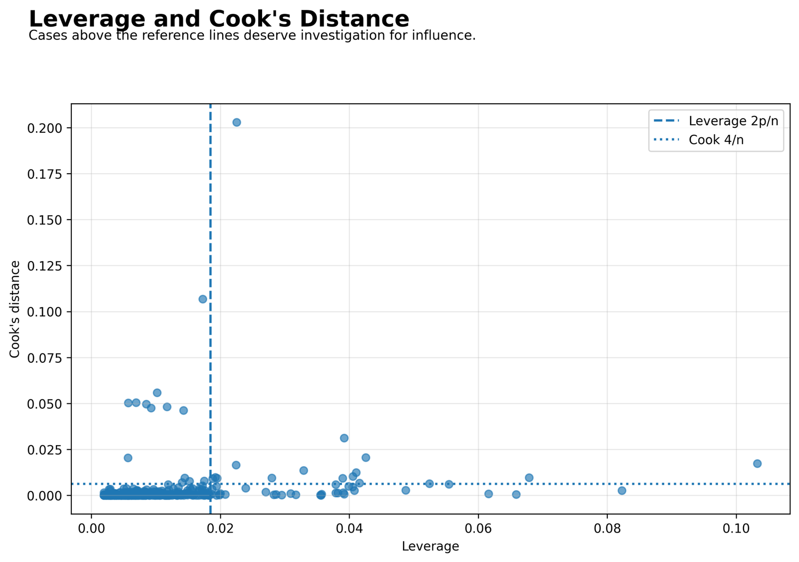
Most records have low leverage and Cook’s distance, while a smaller group deserves case-level review.
The supplied case ledger records predicted values, standardized and deleted residuals, leverage, Cook’s distance and DFFITS.
Influence can alter coefficients and selection membership. It does not automatically identify an invalid record.
Tracing plotted points to source rows separates statistical sensitivity from data correction or deletion decisions.
R Charts and Paired Explanations
The attachment contains four R-labeled chart assets arranged in the exact paired format. No completed R report download is supplied, so these visuals should be treated as same-topic cross-check assets rather than proof of a fully archived independent R execution.
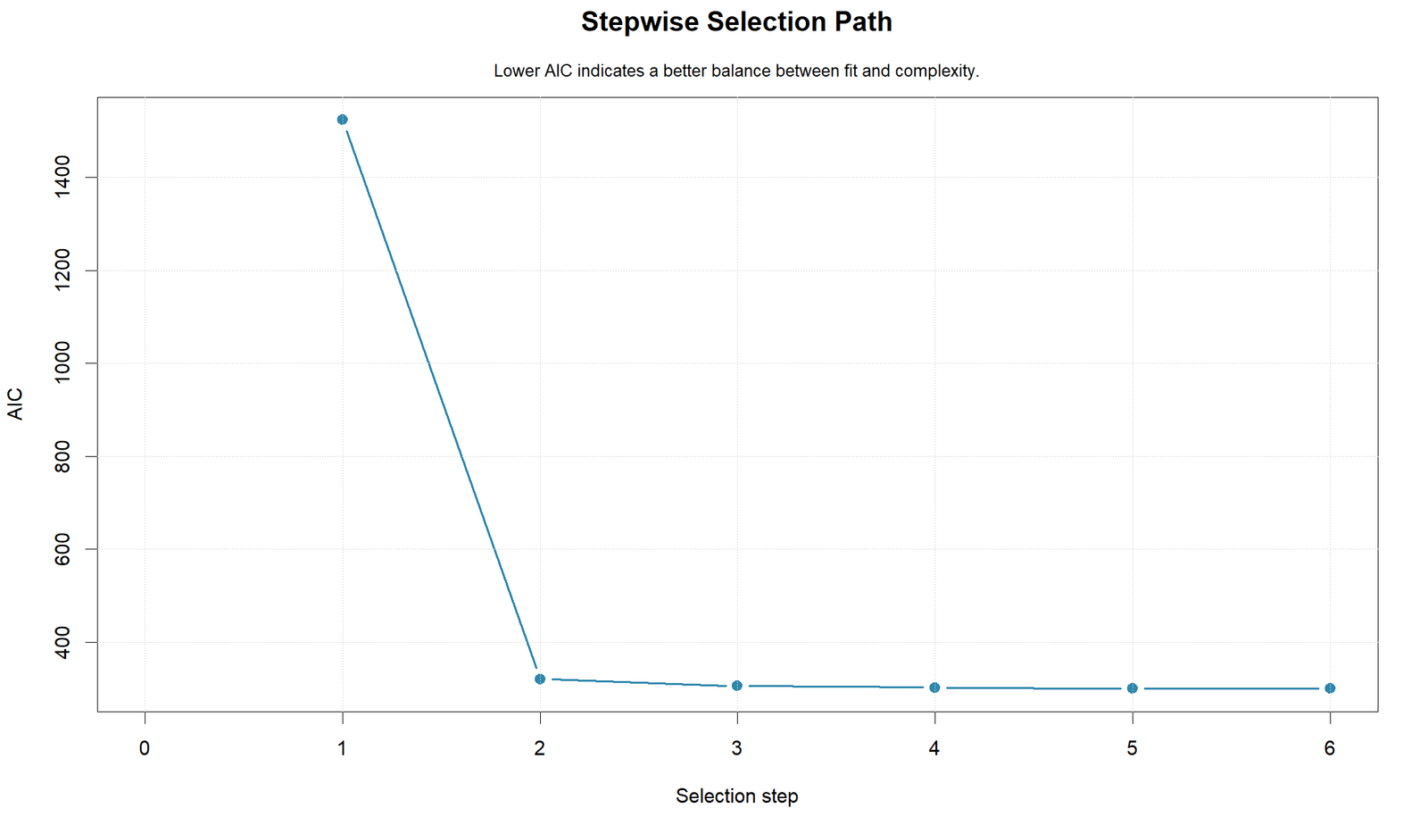
R Chart 1: AIC Selection Path
Pattern: The path should show the same overwhelming first G2 decrease and progressively smaller later moves.
Key values: Verify all six AIC states against 3364.926948, 2162.270813, 2147.309621, 2143.912048, 2141.719377 and 2141.253662.
Interpretation: Agreement requires the same null start, upper scope, direction = both and k = 2.
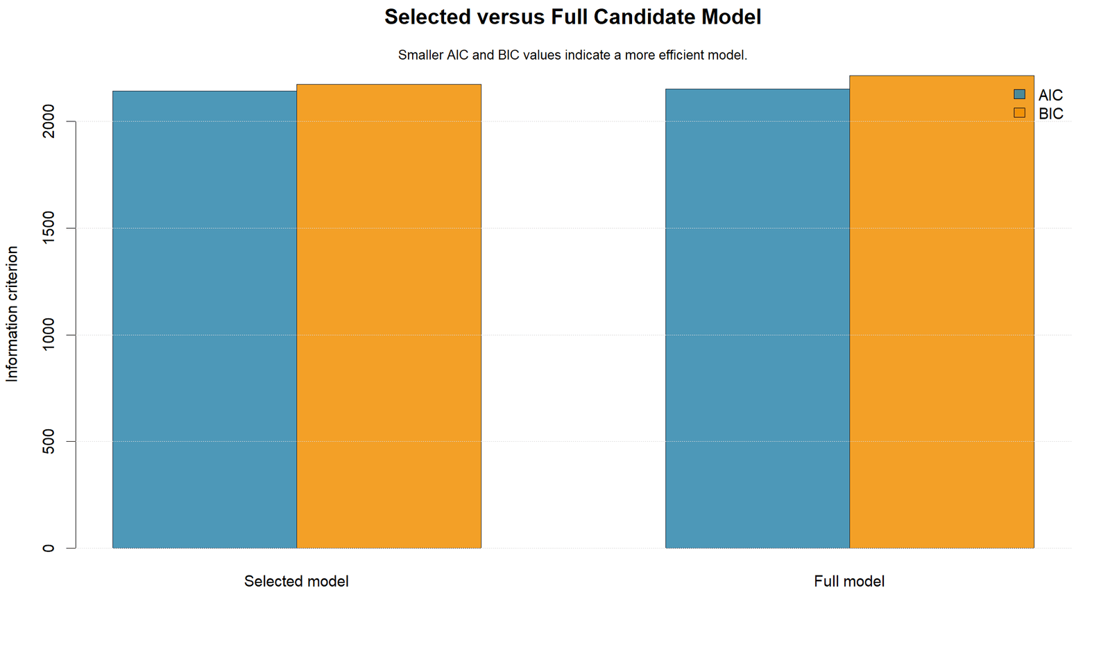
R Chart 2: Selected versus Full Criteria
Pattern: The selected model should have lower AIC and BIC while the full model retains slightly better fitted RMSE.
Key values: Selected AIC/BIC = 2141.253662/2168.106259; full = 2150.218767/2208.399392.
Interpretation: Criteria and prediction error answer different comparison questions.
R Chart 3: Selected Coefficients
Pattern: G2 should dominate, failures should remain negative and the studytime interval should cross zero.
Key values: Reconcile every estimate and interval with the verified coefficient table.
Interpretation: R’s ordinary lm intervals remain post-selection when step chooses the formula on the same data.
R Chart 4: Observed versus Predicted
Pattern: Fitted values should closely track G3 across the dense central range with larger departures at some boundaries.
Key values: The selected model uses 649 records and reports fitted R-squared 0.850563.
Interpretation: This is in-sample fit after searching, not reserved validation performance.
Stepwise Regression Coefficient and Parameter Interpretation
Selected Equation
G2 is the dominant selected slope. Holding the other four selected variables constant, one additional G2 point is associated with approximately 0.885709 additional fitted G3 points. Its ordinary endpoint interval is [0.8191, 0.9523].
G1 remains positive after G2 enters, with B = 0.139457. Failures is negative at −0.218290. Absences has a small positive conditional coefficient of 0.023367. Studytime is positive at 0.096699 but has an ordinary interval crossing zero.
The signs are conditional on the adaptively selected formula and raw numeric coding. The absences coefficient must not be described as evidence that increasing absence would improve grades. Selection and correlation can create conditional signs that differ from marginal associations.
The selected model’s overall F statistic is 731.965860 with conventional p approximately 1.326 × 10−262. This describes the final fitted equation under a fixed-model reference and does not adjust for the search.
Predictions, Effects and Model Meaning
A selected-model prediction substitutes G2, G1, failures, absences and studytime into the endpoint equation. For a hypothetical record with G2 = 11, G1 = 10, failures = 0, absences = 4 and studytime = 2:
The value 11.269045 is a point prediction on the G3 scale. It is not a probability and is not automatically restricted to the observed score range. Rounded coefficients can produce small differences from the saved full-precision prediction.
The supplied case ledger contains 310 source rows rather than all 649 observations. Those available rows are preserved as CSV in the rewrite ZIP. The article does not represent the partial ledger as a complete exported prediction table.
Stepwise Regression Assumptions and Diagnostics
The final selected linear equation still requires an adequate conditional mean and correctly coded terms.
Independent observations are required unless clustering, repeated measures or time dependence are modeled.
Diagnostics assess the endpoint fit but do not erase uncertainty created by searching the same outcomes.
Residual Shape
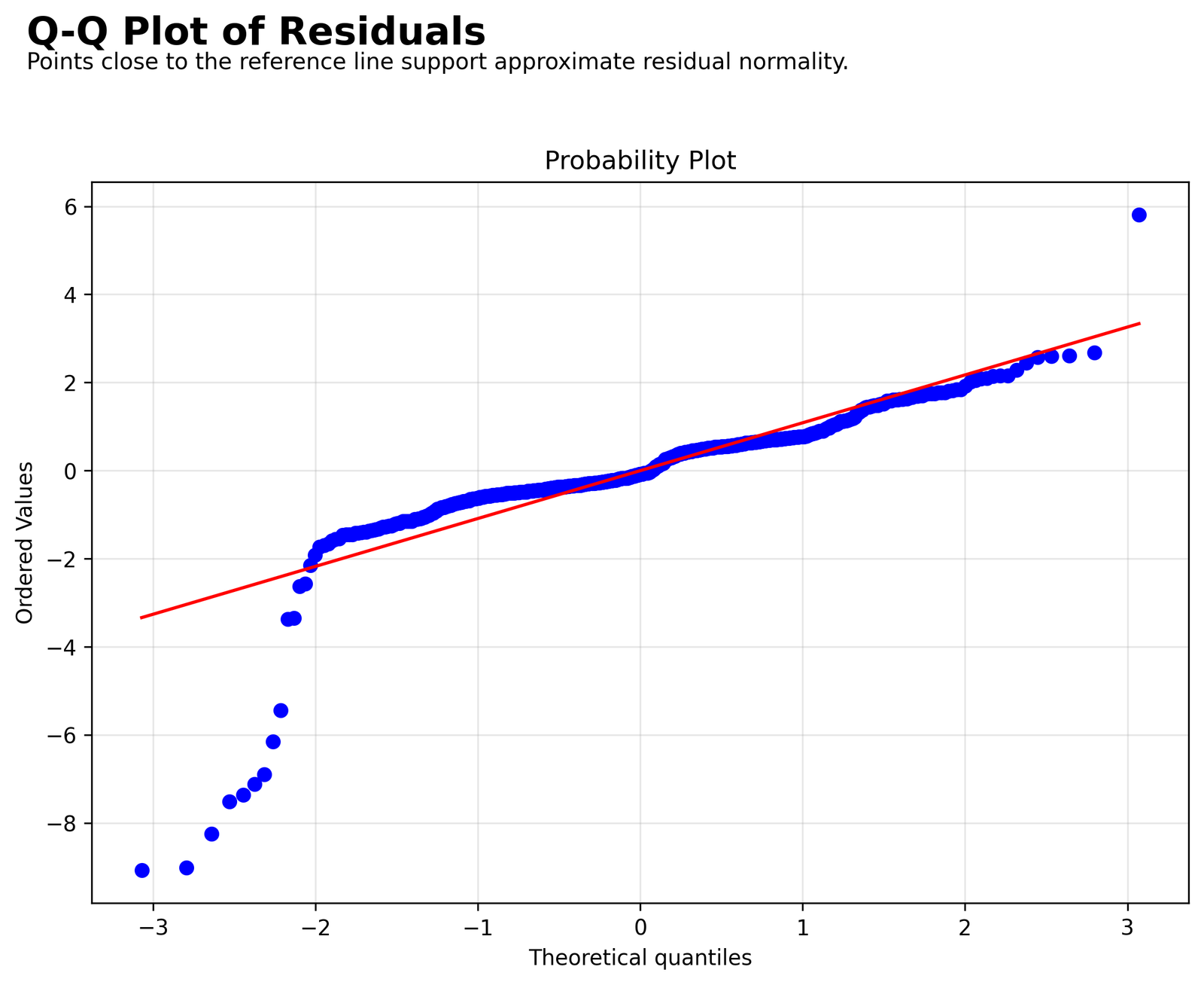
Residual-versus-fitted, histogram and Q-Q evidence should be read together. AIC selection does not guarantee normal errors, constant variance or correct linear form. The Q-Q Plot Normality Check and Regression Diagnostics guides provide broader interpretation.
Serial Dependence
Durbin-Watson is 1.857347, close to two for the supplied row order. This does not replace design knowledge and should not be treated as a universal independence test for unordered student records.
Multicollinearity
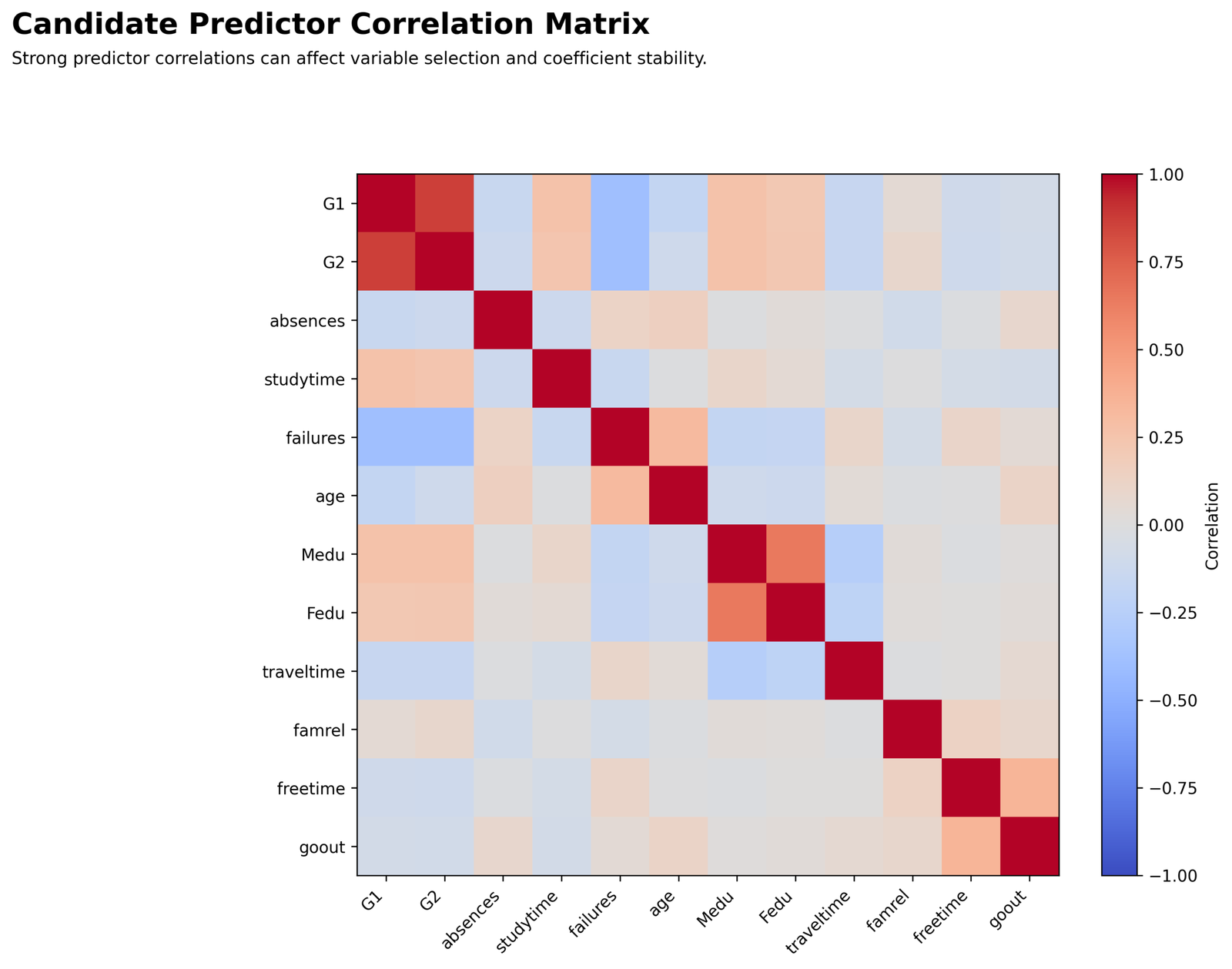
G1 VIF = 4.077721 and G2 VIF = 4.028316. Remaining selected VIF values range from 1.034455 to 1.197793. The grade predictors overlap meaningfully and may exchange coefficient magnitude or selection order under resampling.
Influence
Leverage, Cook’s Distance, deleted residual and DFFITS should be traced to source cases. An influential record can change path membership without being erroneous.
Validation and Stability
The current files provide one deterministic path for 649 rows and no bootstrap inclusion-frequency table. Repeated nested cross-validation or bootstrap selection is needed to quantify how often each term is retained.
Stepwise Regression in Python, R, SPSS and Excel
Python
Python supplies the authoritative saved both-direction AIC path and the ten source chart assets.
- Intercept-only start
- Twelve-term upper scope
- Add and drop neighbors at each step
- Stop when no AIC decrease remains
R
R can reproduce an AIC path with step when null, upper scope, direction and k = 2 are fixed.
- Use the same 649 complete rows.
- Record
selected$anova. - Do not infer full R verification from chart files alone.
SPSS
Standard SPSS STEPWISE linear regression commonly uses probability entry and removal thresholds.
- Name PIN and POUT.
- Do not call the path AIC-based without a custom procedure.
- Fit the verified five-term equation directly for audit.
Excel
The workbook can audit Gaussian AIC, BIC, fitted values and recorded path states.
- Keep all candidate models on identical rows.
- Update parameter counts correctly.
- Label manual work as a saved-path audit.
Code and Formula Panels
Python: both-direction AIC Stepwise Regression
from pathlib import Path
import itertools

import numpy as np
import pandas as pd
import statsmodels.api as sm

DATA = Path("dataset.csv")
OUTCOME = "G3"
CANDIDATES = [
    "G1", "G2", "absences", "studytime", "failures", "age",
    "Medu", "Fedu", "traveltime", "famrel", "freetime", "goout"
]
TOL = 1e-10

raw = pd.read_csv(DATA)
df = raw[[OUTCOME] + CANDIDATES].dropna().copy()


def fit_terms(terms):
    X = sm.add_constant(df[list(terms)], has_constant="add")
    return sm.OLS(df[OUTCOME], X).fit()


def both_direction_aic(candidates):
    selected = []
    current = fit_terms(selected)
    path = [{
        "step": 0,
        "action": "start",
        "term": "intercept only",
        "aic": current.aic,
        "bic": current.bic,
        "adjusted_r_squared": current.rsquared_adj,
        "terms": ""
    }]

    step = 0
    while True:
        proposals = []

        # One-term additions.
        for term in candidates:
            if term not in selected:
                terms = selected + [term]
                fit = fit_terms(terms)
                proposals.append((fit.aic, "add", term, terms, fit))

        # One-term removals. The intercept is never removed.
        for term in selected:
            terms = [x for x in selected if x != term]
            fit = fit_terms(terms)
            proposals.append((fit.aic, "drop", term, terms, fit))

        if not proposals:
            break

        best_aic, action, term, best_terms, best_fit = min(
            proposals, key=lambda x: x[0]
        )

        if best_aic >= current.aic - TOL:
            break

        step += 1
        delta = best_aic - current.aic
        selected = list(best_terms)
        current = best_fit
        path.append({
            "step": step,
            "action": action,
            "term": term,
            "aic": best_fit.aic,
            "delta_aic": delta,
            "bic": best_fit.bic,
            "r_squared": best_fit.rsquared,
            "adjusted_r_squared": best_fit.rsquared_adj,
            "terms": " + ".join(selected)
        })

    return selected, current, pd.DataFrame(path)


selected_terms, selected_model, path = both_direction_aic(CANDIDATES)
full_model = fit_terms(CANDIDATES)

pred = selected_model.predict()
resid = df[OUTCOME] - pred
rmse = float(np.sqrt(np.mean(resid ** 2)))
mae = float(np.mean(np.abs(resid)))

comparison = pd.DataFrame([
    {
        "model": "selected",
        "n": int(selected_model.nobs),
        "terms": " + ".join(selected_terms),
        "r_squared": selected_model.rsquared,
        "adjusted_r_squared": selected_model.rsquared_adj,
        "aic": selected_model.aic,
        "bic": selected_model.bic,
        "rmse": rmse,
        "mae": mae,
    },
    {
        "model": "full candidate model",
        "n": int(full_model.nobs),
        "terms": " + ".join(CANDIDATES),
        "r_squared": full_model.rsquared,
        "adjusted_r_squared": full_model.rsquared_adj,
        "aic": full_model.aic,
        "bic": full_model.bic,
        "rmse": float(np.sqrt(np.mean(full_model.resid ** 2))),
        "mae": float(np.mean(np.abs(full_model.resid))),
    }
])

coef = pd.DataFrame({
    "term": selected_model.params.index,
    "B": selected_model.params.values,
    "SE": selected_model.bse.values,
    "t": selected_model.tvalues.values,
    "p": selected_model.pvalues.values,
    "ci_low": selected_model.conf_int()[0].values,
    "ci_high": selected_model.conf_int()[1].values,
})

influence = selected_model.get_influence()
case_evidence = df.copy()
case_evidence["predicted"] = pred
case_evidence["residual"] = resid
case_evidence["standardized_residual"] = influence.resid_studentized_internal
case_evidence["deleted_residual"] = influence.resid_studentized_external
case_evidence["leverage"] = influence.hat_matrix_diag
case_evidence["cook_distance"] = influence.cooks_distance[0]
case_evidence["dffits"] = influence.dffits[0]

path.to_csv("stepwise_selection_path.csv", index=False)
comparison.to_csv("stepwise_selected_vs_full.csv", index=False)
coef.to_csv("stepwise_selected_coefficients.csv", index=False)
case_evidence.to_csv("stepwise_case_evidence.csv", index=False)

print("Selected terms:", selected_terms)
print(path.to_string(index=False))
print(comparison.to_string(index=False))
print(coef.to_string(index=False))
The function records the intercept-only state, every accepted move and selected-versus-full evidence.
R: AIC selection with step
dat <- read.csv("dataset.csv", check.names = FALSE)

outcome <- "G3"
candidates <- c(
  "G1", "G2", "absences", "studytime", "failures", "age",
  "Medu", "Fedu", "traveltime", "famrel", "freetime", "goout"
)

model_dat <- dat[
  complete.cases(dat[c(outcome, candidates)]),
  c(outcome, candidates)
]

null_model <- lm(G3 ~ 1, data = model_dat)
full_model <- lm(
  G3 ~ G1 + G2 + absences + studytime + failures + age +
    Medu + Fedu + traveltime + famrel + freetime + goout,
  data = model_dat
)

# k = 2 requests ordinary AIC rather than BIC.
selected <- step(
  object = null_model,
  scope = list(lower = formula(null_model), upper = formula(full_model)),
  direction = "both",
  k = 2,
  trace = 1
)

selected_formula <- formula(selected)
selected_summary <- summary(selected)
selection_path <- selected$anova

pred <- predict(selected, newdata = model_dat)
resid <- model_dat$G3 - pred
rmse <- sqrt(mean(resid^2))
mae <- mean(abs(resid))

comparison <- data.frame(
  model = c("selected", "full candidate model"),
  n = c(nobs(selected), nobs(full_model)),
  r_squared = c(summary(selected)$r.squared, summary(full_model)$r.squared),
  adjusted_r_squared = c(
    summary(selected)$adj.r.squared,
    summary(full_model)$adj.r.squared
  ),
  aic = c(AIC(selected), AIC(full_model)),
  bic = c(BIC(selected), BIC(full_model)),
  rmse = c(rmse, sqrt(mean(residuals(full_model)^2))),
  mae = c(mae, mean(abs(residuals(full_model))))
)

coef_table <- data.frame(
  term = rownames(coef(selected_summary)),
  coef(selected_summary),
  row.names = NULL,
  check.names = FALSE
)

write.csv(selection_path, "stepwise_r_selection_path.csv", row.names = FALSE)
write.csv(comparison, "stepwise_r_selected_vs_full.csv", row.names = FALSE)
write.csv(coef_table, "stepwise_r_coefficients.csv", row.names = FALSE)

print(selected_formula)
print(selection_path)
print(comparison)
print(coef_table)
Exact agreement requires identical rows and software likelihood conventions. Preserve the printed anova path.
SPSS: probability-based comparison and selected-model audit
* SPSS standard STEPWISE regression is probability-based,
* not the same algorithm as the verified both-direction AIC search.

REGRESSION
 /MISSING LISTWISE
 /STATISTICS COEFF OUTS R ANOVA CHANGE CI(95) COLLIN TOL
 /CRITERIA=PIN(.05) POUT(.10)
 /DEPENDENT G3
 /METHOD=STEPWISE
   G1 G2 absences studytime failures age Medu Fedu
   traveltime famrel freetime goout
 /SAVE PRED RESID ZRESID SRESID COOK LEVER.

* Fit the verified Python-selected equation directly for auditing.
REGRESSION
 /MISSING LISTWISE
 /STATISTICS COEFF OUTS R ANOVA CI(95) COLLIN TOL
 /DEPENDENT G3
 /METHOD=ENTER G2 G1 failures absences studytime
 /SAVE PRED RESID ZRESID SRESID COOK LEVER.

* Interpretation rule:
* - Name the SPSS PIN and POUT thresholds.
* - Do not label the SPSS path AIC-based unless an extension or custom
*   procedure explicitly calculates and minimizes AIC.
* - An identical final formula does not prove identical search logic.
The standard SPSS command is a related selection procedure, not an automatic reproduction of Python AIC search.
Excel: AIC, BIC, fit and path-audit formulas
Excel audit formulas for Gaussian linear models

Assume:
- n = number of complete rows
- k = number of estimated parameters including the intercept
- SSE = SUMXMY2(ObservedRange, PredictedRange)

Exact Gaussian AIC under the common OLS convention:
=n*(LN(2*PI())+1+LN(SSE/n))+2*k

Gaussian BIC:
=n*(LN(2*PI())+1+LN(SSE/n))+k*LN(n)

R-squared:
=1-SSE/DEVSQ(ObservedRange)

Adjusted R-squared:
=1-(1-R2)*(n-1)/(n-k)

RMSE using the fitted-sample n denominator:
=SQRT(SSE/n)

MAE:
=AVERAGE(ABS(ObservedRange-PredictedRange))

Candidate move:
=Candidate_AIC-Current_AIC

Accept an AIC move only when:
=Candidate_AIC<Current_AIC

Selected-model prediction:
=-0.155190+0.885709*G2+0.139457*G1
 -0.218290*failures+0.023367*absences
 +0.096699*studytime

Important:
- Every candidate model must use the same complete rows.
- k changes whenever a slope enters or leaves.
- Manual cell comparison is an audit of a saved path unless every valid
  addition and removal is refitted at every step.
Use full-precision values and a fixed analysis sample for every candidate comparison.
Advanced Stepwise Regression Topics
These 26 panels extend the worked path from criterion calculation to selection stability, post-selection inference, software differences and responsible reporting.
1. Stepwise Regression Estimand and Research Question
Stepwise Regression is an algorithm for choosing a formula from a declared candidate family. The fitted coefficients describe the selected equation, while the selection estimand is the model favored by the implemented criterion and path rules in the observed sample.
State whether the purpose is exploratory screening, parsimony, prediction or construction of a provisional explanatory model. Selection is not a substitute for a scientific estimand or a causal design.
2. Candidate-Set Definition in Stepwise Regression
The search can consider only G1, G2, absences, studytime, failures, age, Medu, Fedu, traveltime, famrel, freetime and goout. Interactions, nonlinear terms and unmeasured variables are outside the algorithm.
The candidate pool should be justified before the search. Adding terms after reading the first path changes the model family and requires a new validation cycle.
3. Intercept-Only Starting Model in Stepwise Regression
The verified Python path begins with the outcome mean as the only fitted value. Its AIC is 3364.926948 and its R-squared is effectively zero by construction.
Publishing the baseline makes every later AIC change auditable. A different starting model can produce a different greedy path.
4. Both-Direction Search in Stepwise Regression
At each step the algorithm evaluates every valid one-term addition and every valid one-term removal from the current model. It accepts the candidate with the lowest AIC only when the criterion decreases.
Both-direction search is not the same as forward-only selection or backward elimination. Direction, scope, start model and stopping tolerance must be reported.
5. AIC Formula and Parameter Count in Stepwise Regression
AIC equals minus twice the maximized log-likelihood plus twice the number of estimated parameters. For Gaussian OLS, the parameter count includes the intercept and the residual-variance parameter under the software likelihood convention.
Exact absolute AIC values can differ when software counts constants or parameters differently. Candidate rankings should agree only when the same likelihood and convention are used.
6. AIC versus BIC in Stepwise Regression
AIC targets expected out-of-sample information loss and uses a 2k penalty. BIC uses k log(n), which is stronger when n exceeds about 7.4 and often favors smaller models.
The selected five-term model has lower AIC and BIC than the full twelve-term model, but the search itself was driven by AIC. BIC should be reported as a comparison rather than retroactively substituted as the search rule.
7. Same-Sample Requirement in Stepwise Regression
AIC values are comparable only when candidate models use the same outcome observations and likelihood. All verified steps use 649 complete records.
When missingness changes the sample across formulas, an AIC decrease can reflect different rows rather than a better term set. Freeze the analysis sample before searching.
8. First Addition of G2 in Stepwise Regression
Adding G2 lowers AIC from 3364.926948 to 2162.270813, a reduction of 1202.656135. Adjusted R-squared rises to 0.843489.
The enormous first change shows that recent grade history dominates the supplied candidate family. Entry order is criterion-driven and is not a causal hierarchy.
9. Second Addition of G1 in Stepwise Regression
G1 lowers AIC by 14.961192 to 2147.309621 and raises adjusted R-squared to 0.847290 after G2 is already present.
G1 retains incremental predictive information, but its overlap with G2 is reflected in VIF values near four. Resampling may change coefficient size or entry order.
10. Addition of Failures in Stepwise Regression
Failures reduces AIC by 3.397573 to 2143.912048 and produces a final negative coefficient of -0.218290.
The final slope is conditional on G2, G1, absences and studytime. The search step does not establish that failures cause the predicted grade difference.
11. Addition of Absences in Stepwise Regression
Absences lowers AIC by 2.192671 to 2141.719377. Its final coefficient is 0.023367 with a conventional 95 percent interval from 0.002171 to 0.044562.
The positive conditional sign differs from a possible marginal pattern and therefore deserves cautious wording. Selection, correlation and coding all affect the coefficient.
12. Final Addition of Studytime in Stepwise Regression
Studytime lowers AIC by only 0.465715 to 2141.253662 even though its final ordinary p-value is 0.118199.
AIC and p-values optimize different criteria. The term should not be deleted after selection merely to force every displayed p-value below 0.05.
13. Interpreting Small Delta AIC in Stepwise Regression
The final AIC reduction is below one, which indicates weak separation between the four-term and five-term candidates under the observed sample.
Small improvements are especially vulnerable to sampling variation. Bootstrap inclusion frequency or repeated nested validation should be used before calling studytime a stable selected predictor.
14. Selected versus Full Candidate Model in Stepwise Regression
The selected model retains five slopes and has AIC 2141.253662 and BIC 2168.106259. The full model has AIC 2150.218767 and BIC 2208.399392.
The full model has slightly higher R-squared and lower fitted RMSE, while the selected model is more parsimonious. No single metric establishes universal superiority.
15. Greedy Search Limitation in Stepwise Regression
Stepwise Regression follows locally best moves from the current model. It does not automatically examine all 2^12 possible subsets or guarantee the globally lowest-AIC subset.
A different starting point or path constraint can produce another result. Best-subset, penalized and theory-defined alternatives provide useful sensitivity comparisons.
16. Best-Subset Comparison in Stepwise Regression
An exhaustive subset procedure evaluates every allowed combination at each model size. With twelve candidates, 4096 subsets are computationally manageable, but the inferential and validation problems remain.
Finding a globally best in-sample AIC does not make post-selection p-values confirmatory. The entire subset search must still be repeated inside resampling.
17. Correlated Candidates and VIF in Stepwise Regression
Selected VIF is 4.077721 for G1 and 4.028316 for G2. The other selected terms range from 1.034455 to 1.197793.
These values indicate meaningful overlap but not exact linear dependence. Correlated variables can substitute for one another and make selected membership unstable.
18. Post-Selection Coefficient Inference in Stepwise Regression
The final t tests and confidence intervals treat the five-term formula as fixed. They do not account for the many candidate equations inspected on the same outcomes.
Label them as conventional post-selection summaries. Strong confirmatory claims require independent data, sample splitting or a valid selective-inference method.
19. Bootstrap Selection Stability in Stepwise Regression
A bootstrap stability analysis repeats the complete both-direction search in each resample and records inclusion frequency, entry order, coefficient sign and out-of-bag error.
G2 is expected to be highly stable because its AIC gain is enormous. Studytime may be less stable because its final AIC gain is only 0.465715.
20. Nested Cross-Validation in Stepwise Regression
Predictive validation must place candidate screening, AIC search and coefficient fitting inside each training fold. The outer validation fold evaluates the complete selected pipeline.
Selecting variables once on all 649 records and cross-validating only the final formula leaks outcome information and understates selection uncertainty.
21. Nonlinearity and Interactions in Stepwise Regression
The supplied candidate family contains main effects on raw numeric scales. Stepwise Regression cannot discover curvature or interactions that were never offered.
Residual evidence should guide a scientifically defined expanded candidate family, followed by a completely new selection and validation process.
22. Missing Data and Eligibility in Stepwise Regression
The verified path uses 649 complete observations. Complete-case selection is transparent but relies on assumptions about why incomplete rows are absent.
If imputation is used, it must be performed inside resampling. Candidate formulas must continue to use identical rows within each selection comparison.
23. Categorical Coding and Hierarchy in Stepwise Regression
Categorical variables require a fixed indicator scheme and reference category. Multi-column terms should often enter or leave as a group rather than as unrelated dummy columns.
Interactions should respect hierarchy: retaining an interaction while dropping its component main effects may create an equation that is difficult to interpret.
24. SPSS Criterion Difference in Stepwise Regression
Standard SPSS STEPWISE linear regression normally uses probability-to-enter and probability-to-remove thresholds. That is a different algorithm from the verified AIC search.
An identical final formula does not prove equivalent selection. Report the criterion and thresholds shown in the SPSS output.
25. Excel Path Auditing in Stepwise Regression
Excel can reproduce fitted values, SSE, AIC, BIC and the recorded path when every candidate equation is fitted consistently. It is useful for transparent teaching and audit.
Manual inspection is not a reliable general both-direction engine unless every valid addition and removal is evaluated at each step with the correct parameter count.
26. Stepwise Regression Decision Framework
Begin with a justified candidate set and fixed eligible rows. Record the start model, direction, criterion, every accepted move and the first rejected stopping point.
Compare the selected and full models, diagnose the selected fit, repeat the entire search in validation or bootstrap samples and describe the result as exploratory unless independently confirmed.
APA-Style Reporting
Worked Stepwise Regression Report
A both-direction AIC Stepwise Regression procedure screened twelve candidate predictors of final grade G3 in 649 complete observations. The search began with an intercept-only model and evaluated all valid one-term additions and removals at each state. G2 entered first, reducing AIC from 3364.927 to 2162.271. G1, failures, absences and studytime entered subsequently, producing a final AIC of 2141.254.
The selected five-predictor model explained 85.1% of fitted G3 variation, R² = .851, adjusted R² = .849, F = 731.97, with RMSE = 1.248 and MAE = 0.783. Its AIC and BIC were lower than those of the full twelve-predictor model, although the full model had slightly higher R² and lower fitted RMSE. Endpoint coefficients were G2 B = 0.886, G1 B = 0.139, failures B = −0.218, absences B = 0.023 and studytime B = 0.097.
Because the formula was selected on the same data, coefficient tests and intervals were treated as conventional post-selection summaries. External or nested validation and bootstrap inclusion frequencies were recommended before the selected variable set was described as stable.
Publication Checklist
- State G3 as the outcome.
- List all twelve candidate predictors.
- Report 649 common complete rows.
- Name the intercept-only start.
- Name both-direction search.
- State AIC as the acceptance criterion.
- Publish all six path states.
- Report every AIC change.
- Identify five selected predictors.
- Compare selected and full models.
- Report AIC, BIC, R² and RMSE correctly.
- Label p-values as post-selection.
- Report G1 and G2 VIF values.
- Retain residual and influence checks.
- Explain that SPSS criteria differ.
- Disclose the missing full R report.
- Verify every download and image URL.
- Retain five advertisement placements.
Downloads and Verification Resources
Frequently Asked Questions
What is Stepwise Regression?
Stepwise Regression is an automated model-selection procedure that adds or removes eligible predictors according to a declared criterion. The verified Python workflow uses both-direction AIC search.
What outcome and candidates were used?
G3 is the outcome. The twelve candidates are G1, G2, absences, studytime, failures, age, Medu, Fedu, traveltime, famrel, freetime and goout.
Which predictors were selected by Stepwise Regression?
The final five-term equation contains G2, G1, failures, absences and studytime.
Why did G2 enter first in Stepwise Regression?
Adding G2 reduced AIC by 1202.656135, far more than any later move, because G2 has a strong relationship with final grade G3.
Why did Stepwise Regression select studytime when p = 0.118199?
The search criterion was AIC, not a p-value threshold. Studytime reduced AIC by 0.465715, so the implemented algorithm retained it.
Is a Stepwise Regression model always better than the full model?
No. The selected model has lower AIC and BIC, while the full model has slightly higher R-squared and slightly lower fitted RMSE.
Does Stepwise Regression test every possible subset?
No. Both-direction stepwise search is greedy and follows locally best additions or removals. It may miss another subset with a lower AIC.
Can ordinary p-values be trusted after Stepwise Regression?
They are useful descriptive summaries of the chosen equation, but they are optimistic for confirmatory inference because they ignore the search process.
Should variables omitted by Stepwise Regression be called irrelevant?
No. They were not retained under this candidate set, sample and AIC path. Another sample, coding scheme, interaction set or criterion may select them.
How should Stepwise Regression be cross-validated?
Repeat the entire selection algorithm inside each training fold. Do not select once on all observations and validate only the final equation.
What is the selected Stepwise Regression model AIC?
The selected five-predictor model has AIC 2141.253662 and BIC 2168.106259.
What is the selected Stepwise Regression model fit?
R-squared is 0.850563, adjusted R-squared is 0.849401, fitted RMSE is 1.247913 and MAE is 0.782996 for 649 observations.
Is multicollinearity severe?
G1 and G2 have VIF values near four, showing meaningful overlap. The remaining selected terms have VIF values close to one.
Are the supplied R charts a complete R verification?
The attachment provides four R-labeled chart assets but no completed R report download. They should be treated as visual companions unless the full R execution files are supplied.
Is SPSS STEPWISE the same as AIC selection?
Usually not. Standard SPSS STEPWISE uses probability entry and removal rules. The criterion must be named before outputs are compared.
Is Stepwise Regression causal?
No. Variable selection does not remove confounding, selection bias, reverse timing or measurement error. The fitted slopes remain observational associations.
Stepwise Regression Conclusion
The verified both-direction AIC Stepwise Regression path begins with an intercept-only model and selects G2, G1, failures, absences and studytime from twelve candidates. G2 supplies the dominant first improvement, while the final studytime move lowers AIC by only 0.465715.
The selected model reports R² = 0.850563, adjusted R² = 0.849401, AIC = 2141.253662, BIC = 2168.106259, RMSE = 1.247913 and MAE = 0.782996. The full twelve-term model has slightly better fitted R² and RMSE but worse information criteria and seven additional slopes.
The defensible conclusion is about exploratory parsimony within the declared candidate family. Ordinary endpoint tests do not account for selection, unselected variables are not proven irrelevant, and fitted error is not external performance. The next evidence should come from bootstrap stability or nested validation that repeats the complete search.
Correct reporting preserves the candidate set, common sample, start model, direction, criterion, every accepted state, selected-versus-full comparison, diagnostics, software differences and limitations. That transparency is more important than presenting the five-term formula as an automatic final truth.
Stepwise Regression reporting remains credible only when the complete search, endpoint diagnostics and validation limitations are retained together.