Standardized Beta Coefficients: Formula, Interpretation, Confidence Intervals and Examples
Standardized Beta Coefficients place regression slopes on a common standard-deviation scale so predictors measured in grades, counts, years and ordinal categories can be compared inside one model. This worked guide uses 649 complete student records, eight predictors and verified Python, R, SPSS and Excel outputs to separate beta from B, zero-order correlation, partial correlation, semi-partial correlation and unique R-squared contribution.
Standardized Beta Coefficients Model Overview
Standardized Beta Coefficients are unitless partial slopes from a multiple linear regression. They answer a focused question: after the other predictors are held constant, how many standard deviations is the expected outcome predicted to change for a one-standard-deviation increase in a particular predictor? The word standardized refers to scale conversion; it does not refer to stronger assumptions, causal identification or a different fitted outcome.
The method is useful when predictors have unlike units and the analyst needs a within-model comparison. In this example, G1 and G2 are prior grades, studytime is an ordinal study category, failures is a count-like history variable, absences is a count, age is measured in years, and Medu and Fedu are coded parental-education levels. Comparing the original B coefficients alone would mix these units. Standardized Beta Coefficients convert every slope to the same outcome-standard-deviation scale.
The research question is not simply which predictor correlates most strongly with G3. It is which predictor has the strongest conditional linear association with G3 after all eight variables enter together. This distinction matters because G1 and G2 share substantial grade-history information. A simple correlation assigns all shared information to each pair separately, whereas a multiple-regression beta reflects competition among predictors for the same outcome variation.
Use Standardized Beta Coefficients when the outcome is continuous, a linear model is appropriate, the predictors belong in one defensible adjustment set, and scale differences make raw slopes difficult to compare. Do not use the ranking as a substitute for subject-matter importance, causal design, prediction validation or a complete variance decomposition. A large beta can describe a variable that is difficult to change, highly correlated with another measure or close in time and content to the outcome.
The same Standardized Beta Coefficients are obtained by z-scoring the outcome and quantitative predictors before fitting the identical OLS equation. Fitted values, residuals, R², t statistics and p-values do not change; only the coefficient units change. The intercept of the fully standardized equation is approximately zero because all transformed variables are centered.
Standardized Beta Coefficients differ from several neighboring statistics. B is the original-unit slope used for practical prediction. The zero-order correlation is an unadjusted pairwise relationship. Partial correlation controls the other predictors in both variables. Semi-partial, or part, correlation controls the other predictors in the focal predictor only, and its square equals that term’s unique contribution to R² in the fixed model.
The worked model predicts G3 from G1, G2, studytime, failures, absences, age, Medu and Fedu. It uses all 649 complete observations and reports R² = 0.850777, adjusted R² = 0.848912 and F(8, 640) = 456.111097. G2 is the dominant standardized predictor at beta = 0.797983, followed by G1 at beta = 0.121852. Failures and absences have smaller conditional effects, while the intervals for studytime, age, Medu and Fedu include zero.
Quick Answer
What the evidence supports
- G2 has the largest Standardized Beta Coefficient: 0.797983.
- G1 is positive but much smaller: beta = 0.121852.
- Failures is modestly negative: beta = -0.043219.
- Absences is conditionally positive: beta = 0.032697.
- Python and R reproduce the same model and ranking.
What the evidence does not prove
- The largest beta is not automatically the most important cause.
- Small unique contributions do not mean the model explains little overall.
- A sign reversal does not establish a beneficial causal effect.
- Standardization does not repair nonlinearity or heteroscedasticity.
- The ranking is not guaranteed to transfer to another sample.
Table of Contents
- Quick Answer
- Why This Analysis Needs Standardized Beta Coefficients
- How Standardized Beta Coefficients Work
- Variables Used, Coding and Standardization
- Verified Standardized Beta Coefficients Results
- Python Charts and Exact-Value Explanations
- R Charts and Paired Explanations
- Coefficient and Parameter Interpretation
- Predictions, Effects and Model Meaning
- Assumptions and Diagnostics
- Python, R, SPSS and Excel
- Code and Formula Panels
- 26 Advanced Topics
- APA-Style Reporting
- Publication Checklist
- Downloads and Verification Resources
- Related Salar Cafe Guides
- 16 Frequently Asked Questions
- Conclusion
Why This Analysis Needs Standardized Beta Coefficients
The eight predictors are not measured in comparable units. A one-point increase in G2, one additional absence, one year of age and one category increase in parental education are different quantities. The unstandardized slopes are essential for real-unit interpretation, but their numerical sizes cannot be ranked directly as though one unit meant the same thing for every predictor.
Standardized Beta Coefficients solve the scale-comparison problem by expressing each slope relative to the predictor and outcome spread observed in the same sample. The resulting values allow a statement such as “G2 has a larger adjusted standardized association than G1” without pretending that a grade point and an absence are equivalent raw changes.
A simpler correlation analysis would not answer the conditional question because it ignores the other seven predictors. A sequence of separate regressions would also fail because every coefficient would use a different adjustment set. The common multiple-regression equation is therefore necessary before Standardized Beta Coefficients can be compared meaningfully.
The analysis should not use Standardized Beta Coefficients when the outcome requires a different regression family without a clearly defined standardization method, when predictor importance is the primary estimand but shared variance must be allocated, or when causal ranking is the goal. Logistic, Poisson, multilevel and survival models require method-specific effect measures and interpretation.
In this setting, Standardized Beta Coefficients provide the clearest common-scale summary because every predictor remains inside the same adjustment set.
How Standardized Beta Coefficients Work
Original-Unit Regression
OLS first estimates the original-unit coefficients. Each B describes the expected G3-point difference associated with a one-unit predictor increase while the other seven predictors remain fixed. The raw equation generates the fitted values and residuals used in diagnostics.
Scale Conversion
The conversion multiplies the raw slope by the predictor’s sample standard deviation and divides by the outcome’s sample standard deviation. Because the multiplier is positive, the sign, t statistic and p-value are preserved. Confidence limits can be converted with the same multiplier when the observed standard deviations are treated as fixed scaling constants.
Equivalent Fully Standardized Model
Refitting the equation with z-scored variables gives the same Standardized Beta Coefficients and an intercept near zero. The model fit and predictions are unchanged after values are transformed back to the original scale.
Partial, Part and Unique Contribution Formulas
rpartial = t / √(t² + df)
rpart = sign(t)√[t²(1 − R²)/df]
ΔR² = rpart²
Partial correlation removes the remaining predictors from both the focal predictor and G3. Part correlation removes them from the focal predictor only. These quantities add context to Standardized Beta Coefficients because a large beta can coexist with substantial shared variance, while a small beta can still be estimated precisely.
Variables Used, Coding and Standardization
| Role | Variable | Meaning and coding | How it enters | Interpretation caution |
|---|---|---|---|---|
| Outcome | G3 | Final course grade | Continuous response | Standardization expresses effects in G3 SD units, not grade points. |
| Prior grade | G1 | First-period grade | Quantitative predictor | Strong overlap with G2 reduces its unique contribution. |
| Prior grade | G2 | Second-period grade | Quantitative predictor | Closest grade-history measure to G3 and dominant adjusted predictor. |
| Study behavior | studytime | Ordered study-time category | Entered as a numeric linear term | A one-SD change is not necessarily a natural category contrast. |
| Academic history | failures | Number or coded level of prior failures | Numeric predictor | Higher values indicate more failures; sign interpretation depends on coding. |
| Attendance | absences | Recorded absence count | Count-valued predictor in a linear equation | Conditional sign differs from its zero-order correlation. |
| Demographic | age | Age in years | Quantitative predictor | The observed range is narrow, limiting standardized spread. |
| Family education | Medu | Maternal education code | Numeric coded predictor | Ordinal coding assumes an approximately linear step effect. |
| Family education | Fedu | Paternal education code | Numeric coded predictor | Interpret the coding scale, not a literal year-of-education change. |
All Standardized Beta Coefficients use the same 649 complete observations. The outcome definition, predictor coding, intercept, missing-data rule and eight-variable formula are fixed across Python and R. This fixed design is essential: comparing coefficients from different samples or adjustment sets would mix substantive change with scale change.
Verified Standardized Beta Coefficients Results
Model Summary
| N | Predictors | R² | Adjusted R² | F statistic | df | Model p | RMSE |
|---|---|---|---|---|---|---|---|
| 649 | 8 | 0.850777 | 0.848912 | 456.111097 | 8, 640 | 1.455 × 10-258 | 1.255758 |
The equation explains about 85.08% of the observed variance in G3 within this sample. The large F statistic indicates that the eight-predictor model improves substantially over an intercept-only equation. This joint result does not mean that every coefficient is individually large or distinguishable from zero.
Coefficient Evidence
| Predictor | B | SE | t | p | 95% CI for B | Standardized beta |
|---|---|---|---|---|---|---|
| G1 | 0.143397 | 0.036672 | 3.9103 | 0.000102 | [0.0714, 0.2154] | 0.121852 |
| G2 | 0.884807 | 0.034369 | 25.7440 | 7.355 × 10-101 | [0.8173, 0.9523] | 0.797983 |
| studytime | 0.096632 | 0.062091 | 1.5563 | 0.1201 | [-0.0253, 0.2186] | 0.024811 |
| failures | -0.235361 | 0.095234 | -2.4714 | 0.0137 | [-0.4224, -0.0484] | -0.043219 |
| absences | 0.022762 | 0.010919 | 2.0846 | 0.0375 | [0.0013, 0.0442] | 0.032697 |
| age | 0.022685 | 0.043668 | 0.5195 | 0.6036 | [-0.0631, 0.1084] | 0.008554 |
| Medu | -0.044951 | 0.057938 | -0.7759 | 0.4381 | [-0.1587, 0.0688] | -0.015786 |
| Fedu | 0.022025 | 0.059316 | 0.3713 | 0.7105 | [-0.0945, 0.1385] | 0.007499 |
Correlation and Unique-Contribution Evidence
| Predictor | Zero-order r | Partial r | Part r | Unique ΔR² | Interpretation |
|---|---|---|---|---|---|
| G2 | 0.918548 | 0.713255 | 0.393100 | 0.154528 | Largest adjusted and unique contribution. |
| G1 | 0.826387 | 0.152753 | 0.059708 | 0.003565 | Strong raw relation, much smaller unique role after G2. |
| failures | -0.393316 | -0.097227 | -0.037737 | 0.001424 | Negative association attenuated after adjustment. |
| absences | -0.091379 | 0.082122 | 0.031831 | 0.001013 | Conditional sign reversal; interpret cautiously. |
Quick report downloads
Use the software reports to verify the displayed values before publication.
Python Charts and Exact-Value Explanations
The eight Python figures connect Standardized Beta Coefficients to uncertainty, model fit, residual behavior, partial association and unique contribution. Each explanation states the visible pattern, exact values, statistical interpretation and practical reason the chart matters.
Python Chart 1: Standardized Betas with Confidence Intervals
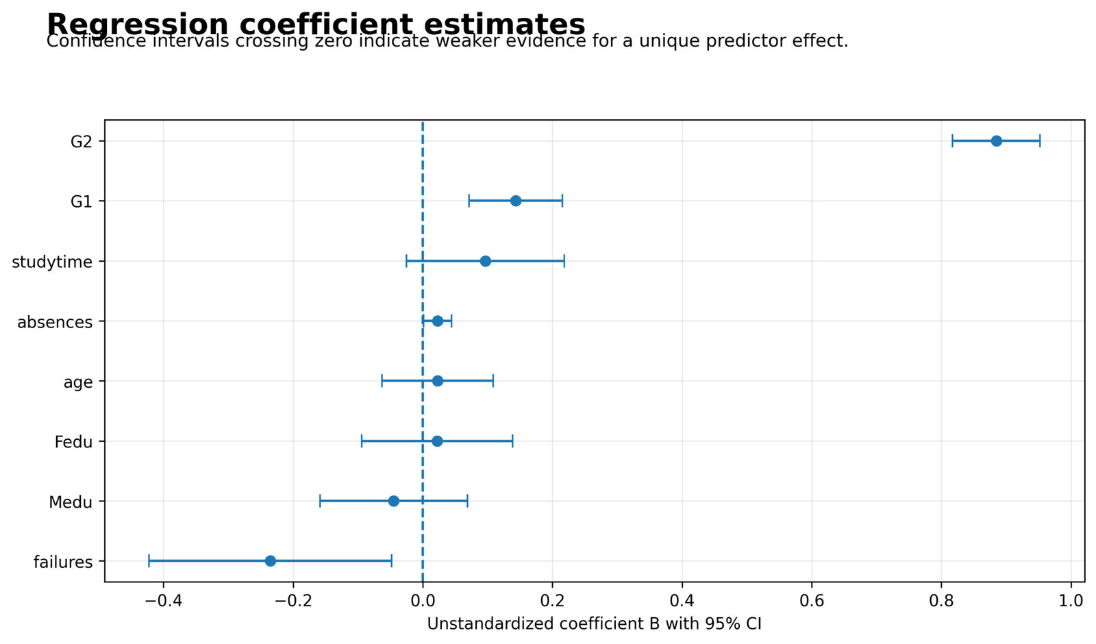
The G2 point and interval sit far to the positive side of the remaining predictors. G1 is positive but much smaller, failures is modestly negative, and the intervals for studytime, age, Medu and Fedu cross zero.
G2 beta = 0.797983 with an approximate standardized 95% interval of 0.7371 to 0.8589. G1 beta = 0.121852 with an interval of about 0.0607 to 0.1830. Failures beta = -0.043219 with an interval of about -0.0776 to -0.0089.
The interval display separates magnitude from precision. G2 is both large and precisely estimated; several small coefficients are too uncertain to support a directional claim after adjustment.
Standardized Beta Coefficients should not be ranked from bar length alone. The uncertainty bands show which apparent differences are stable enough to discuss and which may reflect sampling variation.
Python Chart 2: Absolute Standardized Beta Ranking
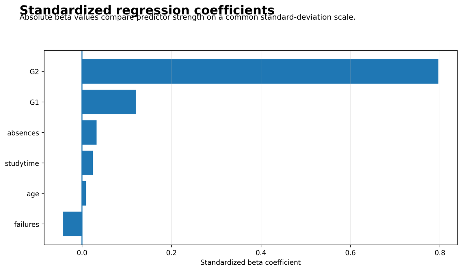
One coefficient dominates the ranking. G2 is followed by G1, while every remaining absolute beta is below 0.044.
G2 = 0.797983; G1 = 0.121852; failures = -0.043219; absences = 0.032697; studytime = 0.024811; Medu = -0.015786; age = 0.008554; Fedu = 0.007499.
The ranking compares conditional slopes after every variable has been placed on a standard-deviation scale. It does not compare simple correlations and it does not allocate shared explained variance.
The chart answers a within-model scale question. It does not establish which variable is the best intervention target, the most important cause, or the most stable predictor in another population.
Python Chart 3: Coefficient P-Value Display
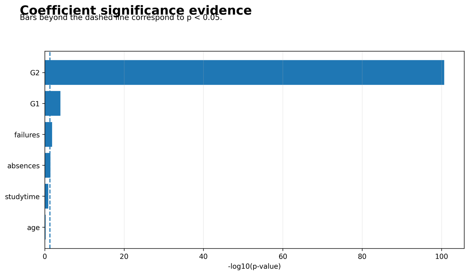
Four predictors fall below the conventional 0.05 line, whereas four do not. The ordering differs from the beta ranking because statistical evidence depends on both effect size and standard error.
G2 p = 7.355 × 10-101; G1 p = 0.000102; failures p = 0.0137; absences p = 0.0375. Studytime p = 0.1201, age p = 0.6036, Medu p = 0.4381 and Fedu p = 0.7105.
Standardizing a coefficient multiplies its estimate and standard error by the same positive factor, so the t statistic and p-value remain unchanged when the transformation is performed consistently.
A p-value chart is an evidence display, not an importance chart. G2 has both a large beta and overwhelming evidence, but a small p-value by itself would not imply practical importance.
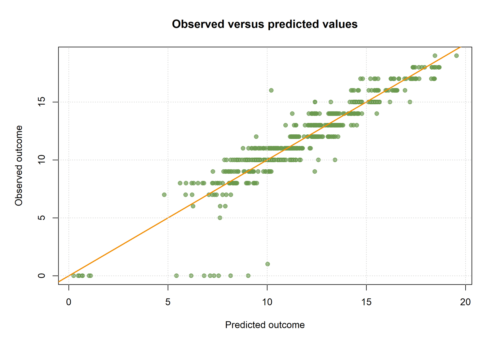
Python Chart 4: Observed versus Predicted G3
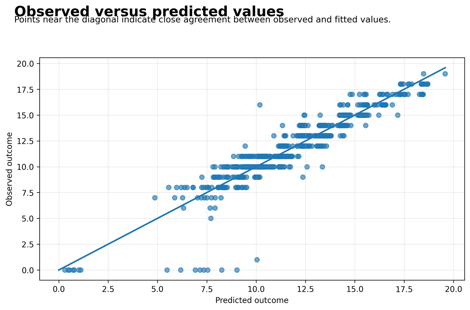
Predictions follow the observed grade pattern closely through the dense middle of the range, while visible vertical deviations remain for some records and near the outcome boundaries.
N = 649, R² = 0.850777, adjusted R² = 0.848912, F(8, 640) = 456.111097 and RMSE = 1.255758. In the source-row audit, a case with G3 = 11 has a fitted value of 9.8327 and residual 1.1673.
The graph evaluates the original regression, not the rescaling step. Standardized Beta Coefficients inherit the fit, strengths and defects of that same equation.
A polished coefficient ranking is not enough if the model predicts poorly or misses systematic structure. Whole-model fit provides the context in which individual standardized effects should be interpreted.
Python Chart 5: Residuals versus Fitted Values
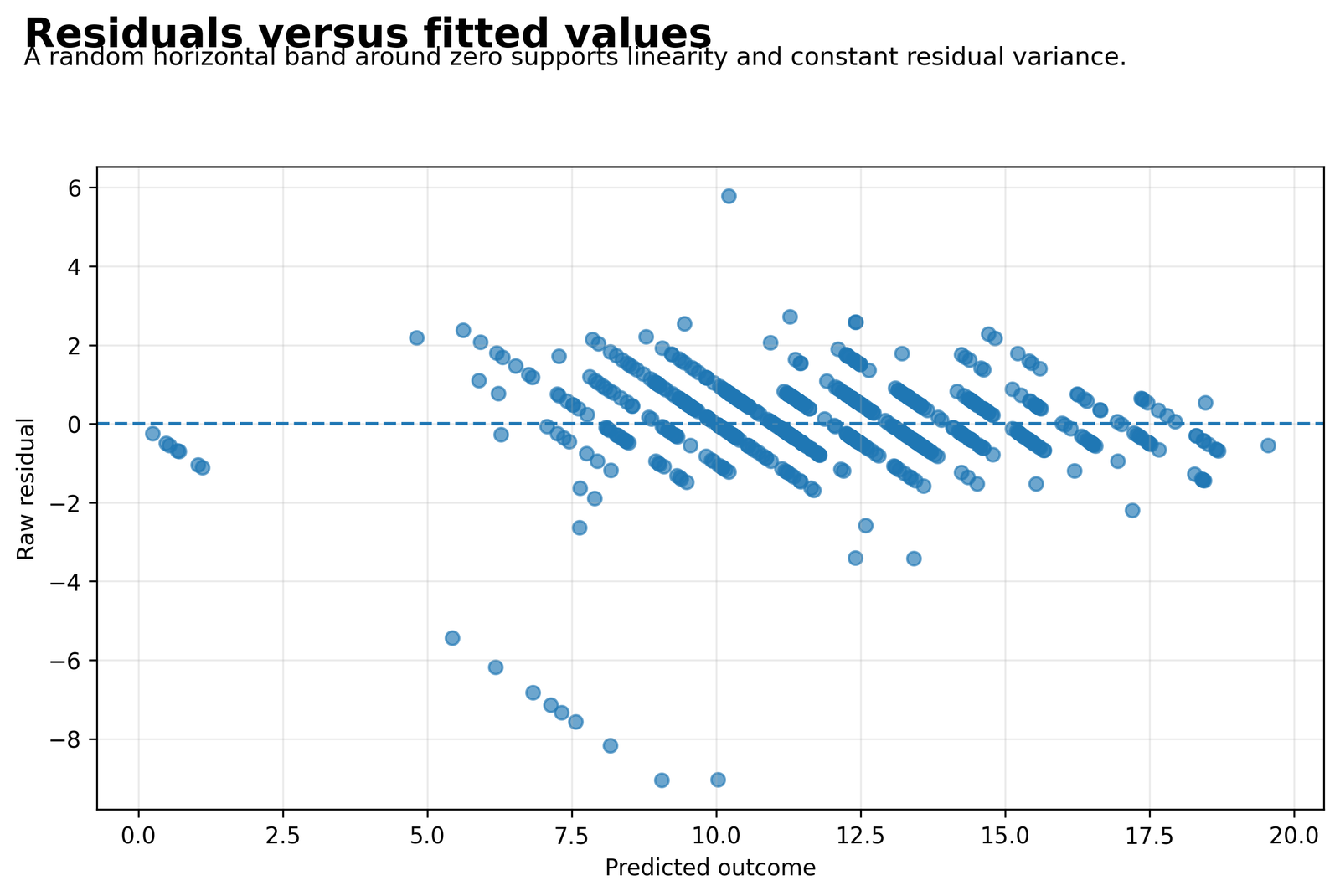
Residuals are centered around zero but form grade-related bands because G3 is recorded in discrete score units. The important diagnostic questions are curvature, changing spread and isolated large errors.
The fitted model has RMSE 1.255758. One audited row has a standardized residual of 0.9855 with leverage 0.1102 and Cook distance 0.01337; another has a raw residual of -1.3693 and standardized residual -1.0966.
Standardizing predictors does not remove heteroscedasticity, nonlinearity or influential observations. Those features belong to the regression error structure and remain present after coefficients are converted to beta.
Residual evidence determines whether conventional intervals and coefficient comparisons are credible. A problematic pattern should be addressed before presenting Standardized Beta Coefficients as stable summaries.
Python Chart 6: Residual Distribution
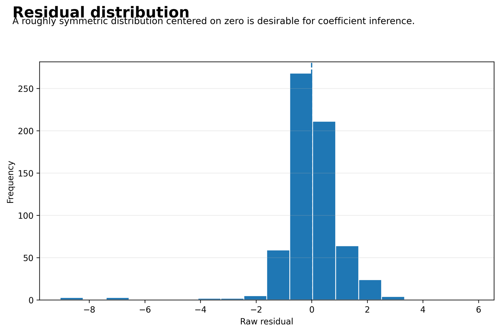
The residual distribution is concentrated near zero with visible tails. OLS with an intercept forces the mean residual to approximately zero, but it does not force symmetry or normality.
The residual standard error and RMSE are approximately 1.255758 for the 649-case model with 640 residual degrees of freedom. The coefficient tests use those residuals and the common design matrix.
Minor non-normality is often less consequential with 649 observations than strong heteroscedasticity, dependence or influence. The distribution should therefore be read with the residual-versus-fitted and case-diagnostic evidence.
Confidence intervals around Standardized Beta Coefficients rely on the same sampling assumptions as intervals around B. Rescaling does not make weak error assumptions disappear.
Python Chart 7: Partial Regression for G2
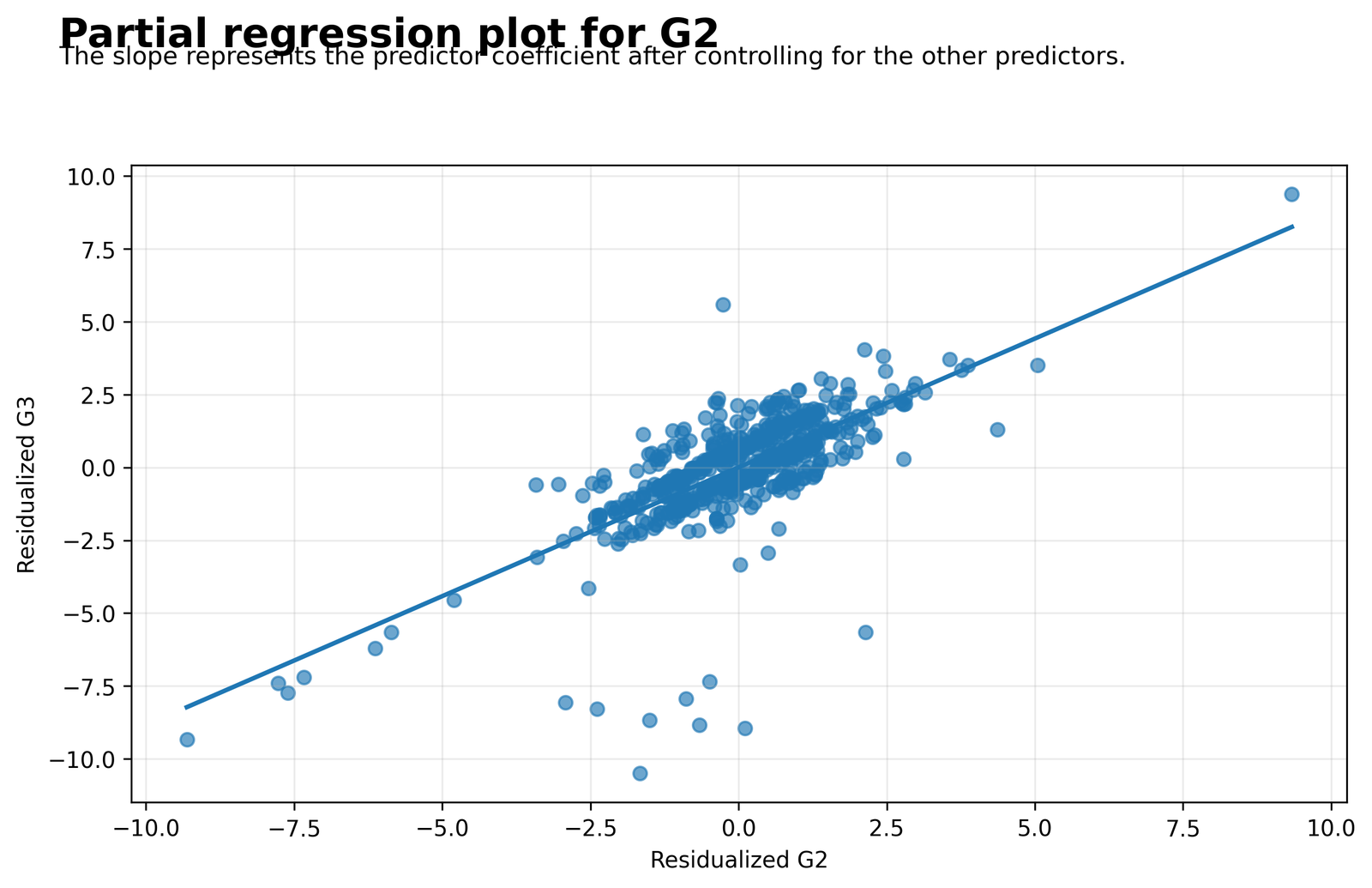
The residualized G2 values and residualized G3 values show a strong positive linear relationship after the other seven predictors are removed from both variables.
G2 has B = 0.884807, beta = 0.797983, t = 25.7440, p = 7.355 × 10-101, partial r = 0.713255 and part r = 0.393100.
The added-variable slope equals the original-unit partial slope for G2. The partial correlation summarizes the residualized association, while beta rescales the slope using the marginal standard deviations of G2 and G3.
This chart shows why G2 remains dominant after adjustment. It also makes clear that the conclusion is conditional on the seven-variable adjustment set rather than a simple bivariate relationship.
Python Chart 8: Correlation and Unique-Contribution Comparison
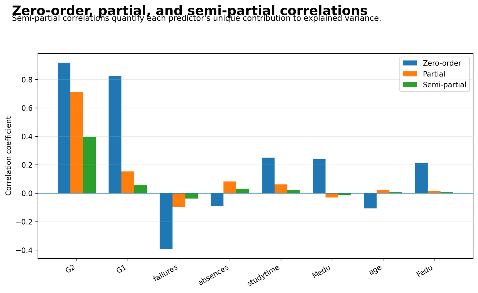
Zero-order relationships shrink substantially after adjustment, especially for the two prior-grade measures. G2 retains the largest partial and semi-partial association, while the unique contributions of most other terms are small.
For G2: zero-order r = 0.918548, partial r = 0.713255, part r = 0.393100 and unique ΔR² = 0.154528. For G1: 0.826387, 0.152753, 0.059708 and 0.003565. Failures contributes 0.001424 uniquely and absences 0.001013.
Standardized Beta Coefficients, partial correlations and part correlations answer related but different questions. The squared part correlation is the single predictor’s incremental R² in this fixed model.
The contrast exposes shared explained variance. Total R² is 0.850777, far larger than the sum of the small unique contributions because correlated predictors explain much of the outcome jointly.
R Charts and Paired Explanations
The R output independently reconstructs the same Standardized Beta Coefficients on the same 649 observations. The four R charts are shown in two paired rows, with the matching explanation directly below each figure on desktop and immediately after each figure on mobile.
(‘\n
\n
\n
\n
\n
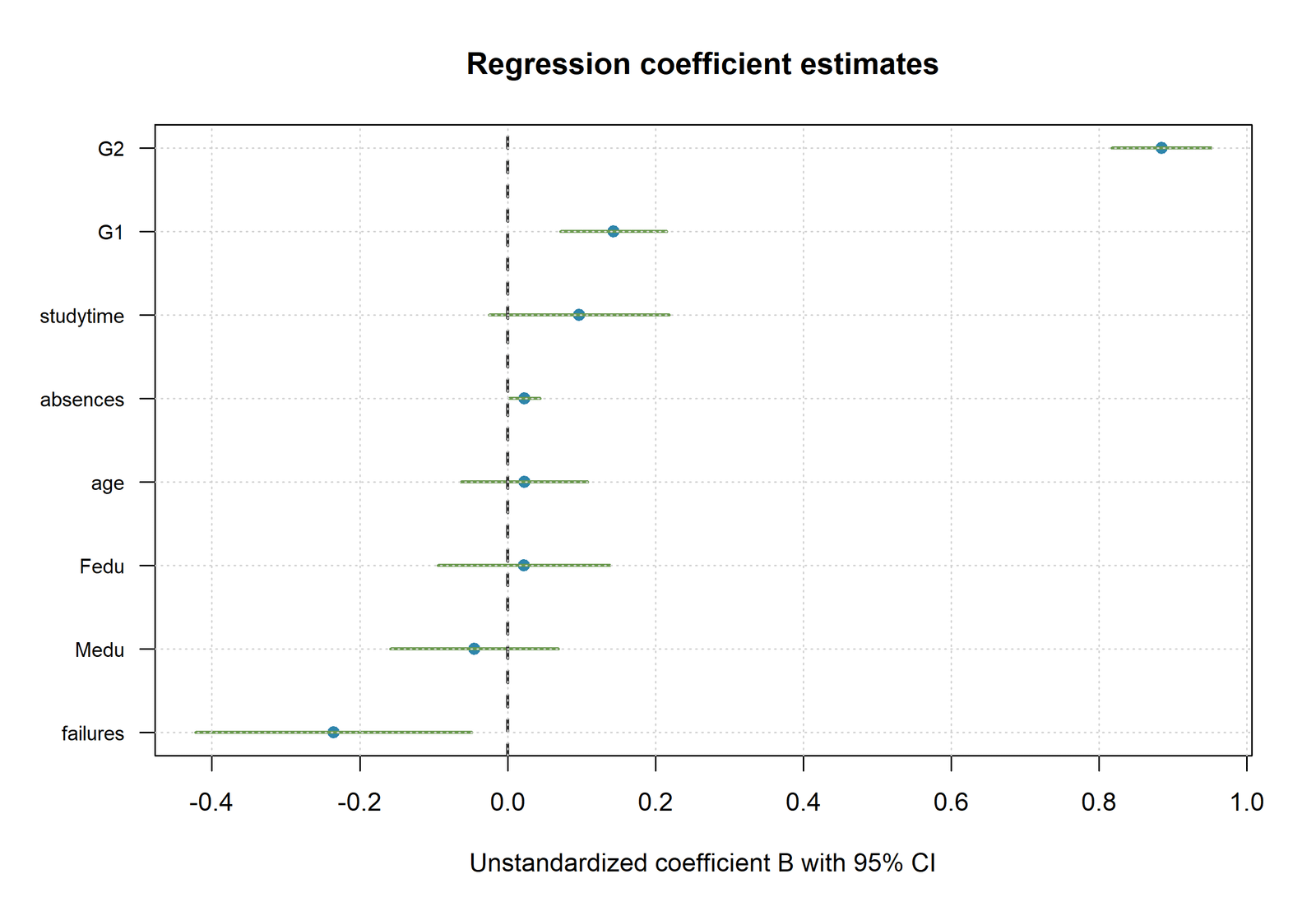
R Chart 1: Standardized Betas with Confidence Intervals
\n
Pattern: G2 is separated clearly from the remaining effects, G1 is a smaller positive effect, and several intervals include zero.
Key values: G2 beta = 0.797983 and G1 beta = 0.121852; the R output reproduces the same model R² = 0.850777 and adjusted R² = 0.848912.
Interpretation: The agreement indicates that the transformation, sample and formula were aligned across Python and R.
\n
\n
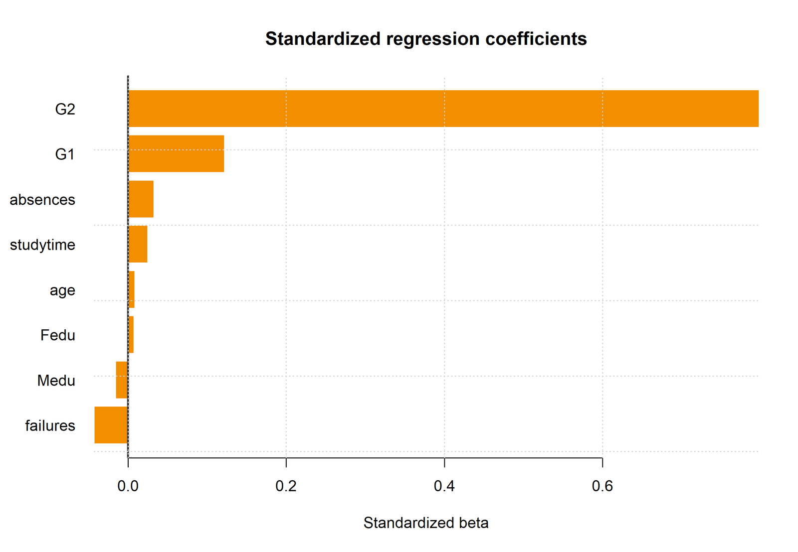
R Chart 2: Standardized Beta Ranking
\n
Pattern: G2 dominates, G1 is a distant second, and all other absolute values are below 0.044.
Key values: The leading values are G2 = 0.797983, G1 = 0.121852, failures = -0.043219 and absences = 0.032697.
Interpretation: The ranking is conditional on the complete eight-predictor model and on sample standard deviations calculated from the same 649 observations.
\n
\n
\n
‘, ‘\n
\n
\n
\n
\n
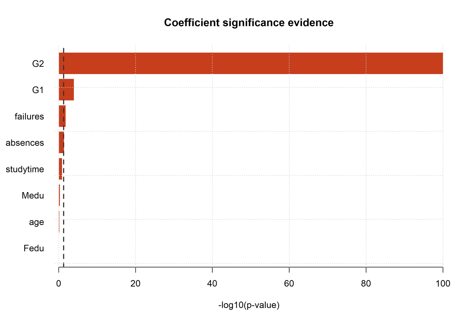
R Chart 3: Coefficient P Values
\n
Pattern: G1, G2, failures and absences are below 0.05; the other four terms are above 0.05.
Key values: The exact p-values are 0.000102 for G1, 7.355 × 10-101 for G2, 0.0137 for failures and 0.0375 for absences.
Interpretation: R and Python agree because standardization preserves each t statistic when the same standard deviations and complete-case sample are used.
\n
\n
R Chart 4: Observed versus Predicted G3
\n
Pattern: Most points follow the reference direction, with remaining prediction error visible around the fitted line and outcome limits.
Key values: N = 649, R² = 0.850777, adjusted R² = 0.848912 and RMSE = 1.255758.
Interpretation: The standardized coefficients do not create different fitted values; they are a re-expression of the same OLS equation.
\n
\n
\n
‘)
Standardized Beta Coefficient and Parameter Interpretation
G2: Strongest Conditional Standardized Association
G2 has B = 0.884807 and beta = 0.797983. In original units, a one-point increase in G2 is associated with an expected 0.885-point increase in G3 while the remaining predictors are fixed. On the standardized scale, a one-SD G2 increase is associated with a 0.798-SD increase in predicted G3.
The 95% B interval from 0.8173 to 0.9523 is entirely positive, and t = 25.7440 with p = 7.355 × 10-101. The partial correlation of 0.713255 and unique ΔR² of 0.154528 confirm that G2 retains a substantial adjusted role after G1 and the other covariates are included.
G1: Positive but Strongly Overlapping with G2
G1 has B = 0.143397, beta = 0.121852 and p = 0.000102. The coefficient remains positive and precisely estimated, but it is far smaller than G2’s standardized effect. The contrast between zero-order r = 0.826387 and part r = 0.059708 shows that most of G1’s predictive information overlaps with the remaining model, especially G2.
Failures and Absences: Small Conditional Effects
Failures is negative, B = -0.235361 and beta = -0.043219, with a B interval from -0.4224 to -0.0484. Absences is positive after adjustment, B = 0.022762 and beta = 0.032697, even though its zero-order correlation is negative. The failures result is modest; the absences sign reversal requires especially careful noncausal language.
Fully Standardized Prediction Equation
The equation predicts G3 in standard-deviation units. Its intercept is approximately zero when every variable is centered and standardized using the same 649 observations. The raw-unit equation remains preferable for practical prediction because users can enter grades, counts and ages directly.
Predictions, Effects and Model Meaning
Standardized Beta Coefficients do not create a second prediction model. They re-express the same fitted equation. A standardized prediction is calculated from the z-scored predictors and the beta equation above. To return to grade points, multiply the predicted z score by SD(G3) and add the G3 mean used in the analysis.
For a one-predictor thought experiment, increasing G2 by one sample standard deviation while holding the other standardized predictors constant changes predicted G3 by 0.797983 outcome standard deviations. This is a conditional model contrast, not a promise for a particular student and not a causal treatment effect.
Prediction accuracy should be evaluated out of sample when the objective is forecasting. The displayed R² and RMSE are in-sample summaries. A validation workflow must recompute means, standard deviations and coefficients inside every training fold to avoid leakage.
Standardized Beta Coefficients Assumptions and Diagnostics
Regression assumptions to inspect
- Approximately linear conditional mean for G3.
- Independent observations under the sampling design.
- Residual spread appropriate for the chosen standard errors.
- No single case or leverage pattern dominating the equation.
- Predictors coded consistently and measured with acceptable reliability.
What standardization does not fix
- Curvature or omitted interactions.
- Heteroscedasticity or clustered dependence.
- Outliers, leverage or data errors.
- Multicollinearity among predictors.
- Confounding and causal identification.
Linearity and Residual Form
The observed-versus-predicted and residual-versus-fitted charts assess the same equation used to calculate Standardized Beta Coefficients. Discrete grade bands are expected, but systematic curvature or a widening residual envelope would indicate that a straight additive model is incomplete.
Normality and Uncertainty
The residual distribution affects normal-theory intervals more than it affects the algebraic beta conversion. With 649 observations, mild tail departure may have limited impact, but robust covariance or bootstrap intervals can be used when heteroscedasticity or influential errors are material.
Multicollinearity
G1 has VIF = 4.164832 and tolerance = 0.240106. G2 has VIF = 4.120795 and tolerance = 0.242672. The values are below the supplied VIF-five review rule, yet they explain why the two prior-grade predictors have strong zero-order correlations but very different unique and standardized contributions.
Influence and Case Review
The fitted-row audit includes predicted values, raw and standardized residuals, leverage and Cook distance. Low residual error does not guarantee low leverage, and a large residual is not automatically a data error. Cases should be checked against source records and the model specification before any exclusion is considered.
Standardized Beta Coefficients in Python, R, SPSS and Excel
Python
Fits the original OLS equation, calculates beta from sample standard deviations, reconstructs partial and part correlations, creates confidence intervals and exports all eight chart stories.
- Keep
ddof=1for sample SDs. - Use the same complete rows for the model and scaling.
- Preserve predictor order and case identifiers.
R
Reproduces the coefficient transformation and same-sample diagnostics independently. Values should agree with Python apart from harmless display rounding.
- Use
model.frame()from the fitted model. - Exclude the intercept from the beta vector.
- Check contrasts and missing-data handling.
SPSS
The REGRESSION Coefficients table displays B and standardized Beta together. Collinearity statistics provide tolerance and VIF for the same predictor set.
- Request coefficients, confidence intervals and collinearity.
- Confirm N = 649 in the Case Processing or model output.
- Match the ENTER predictor list exactly.
Excel
The worked workbook makes the scale conversion transparent with means, sample standard deviations, B values and formulas for beta.
- Use
STDEV.S, notSTDEV.P. - Keep the outcome and predictor ranges aligned.
- Do not round B before calculating beta.
Code and Formula Panels
Python: Fit OLS and calculate Standardized Beta Coefficients
import statsmodels.api as sm

predictors = ["G1", "G2", "studytime", "failures",
              "absences", "age", "Medu", "Fedu"]
model_data = data[["G3", *predictors]].dropna()

X = sm.add_constant(model_data[predictors])
y = model_data["G3"]
fit = sm.OLS(y, X).fit()

sd_x = model_data[predictors].std(ddof=1)
sd_y = y.std(ddof=1)
beta = fit.params[predictors] * sd_x / sd_y

beta_ci = fit.conf_int().loc[predictors].mul(sd_x / sd_y, axis=0)
print(beta)
print(beta_ci)
The calculation uses the exact rows retained by the model and sample standard deviations with denominator n − 1.
R: Reconstruct beta from the fitted model frame
form <- G3 ~ G1 + G2 + studytime + failures +
  absences + age + Medu + Fedu

fit <- lm(form, data = dat, na.action = na.omit)
mf <- model.frame(fit)
y <- model.response(mf)
b <- coef(fit)[-1]

sd_x <- sapply(mf[names(b)], sd)
beta <- b * sd_x / sd(y)
print(beta)
Using the fitted model frame prevents the standard deviations from being calculated on rows excluded by the regression.
SPSS: Request B, Beta, confidence intervals and VIF
REGRESSION
  /DEPENDENT G3
  /METHOD=ENTER G1 G2 studytime failures absences age Medu Fedu
  /STATISTICS COEFF OUTS R ANOVA COLLIN TOL CI(95)
  /RESIDUALS HISTOGRAM(ZRESID) NORMPROB(ZRESID)
  /SAVE PRED RESID ZRESID COOK LEVER.
The SPSS Coefficients table reports the unstandardized B and standardized Beta columns for the same ENTER model.
Excel: Transparent beta, partial r and unique contribution formulas
=B_Coefficient*STDEV.S(Predictor_Range)/STDEV.S(Outcome_Range)

=SIGN(t_value)*SQRT((t_value^2)/(t_value^2+Residual_DF))

=SIGN(t_value)*SQRT((t_value^2*(1-R_Squared))/Residual_DF)

=Part_Correlation^2
The first formula calculates beta. The second calculates partial correlation, the third calculates part correlation and the fourth gives the term’s unique ΔR².
26 Advanced Standardized Beta Coefficients Topics
These advanced panels extend the worked result without changing the central model. Open only the topic needed for interpretation, diagnostics, reporting or software verification.
1. Standardized Beta Coefficients: Standardized Beta Formula and Exact Equivalence
Standardized Beta Coefficients can be obtained by multiplying each original-unit slope by SD(X) and dividing by SD(Y). The same values result when the outcome and all quantitative predictors are converted to z scores before fitting the identical OLS model with an intercept.
This equivalence holds because centering and positive rescaling change the units of the normal equations without changing the underlying fitted values, residuals, R², t statistics or p-values. Minor differences should be limited to rounding or software conventions for standard deviations.
2. Standardized Beta Coefficients: Why G2 Dominates the Standardized Ranking
G2 has beta 0.797983, much larger than G1 at 0.121852 and every remaining absolute beta below 0.044. It is the strongest conditional standardized association in this model because it retains substantial variation related to G3 after the other seven predictors are controlled.
The result is also substantively unsurprising: G2 is a recent grade measure close to the final grade outcome. Strong predictive proximity should not be confused with an intervention effect or with evidence that changing G2 mechanically causes an equal change in G3.
3. Standardized Beta Coefficients: G1 and Shared Grade-History Variance
G1 has a strong zero-order correlation with G3 of 0.826387, yet its beta is only 0.121852 after G2 and six other predictors enter. Its partial correlation is 0.152753 and part correlation is 0.059708.
The reduction does not mean G1 is unimportant in every sense. It means much of the information G1 provides is shared with G2. The joint model assigns the overlapping predictive information according to the geometry of the complete design matrix.
4. Standardized Beta Coefficients: Negative Standardized Effect for Failures
Failures has B = -0.235361, beta = -0.043219, t = -2.4714 and p = 0.0137. Its 95% interval for B runs from -0.4224 to -0.0484, preserving the negative direction after adjustment.
The standardized magnitude is modest even though the coefficient is distinguishable from zero. A one-standard-deviation increase in the failures variable is associated with a 0.043-standard-deviation decrease in predicted G3, holding the other variables fixed.
5. Standardized Beta Coefficients: Absences and Conditional Sign Reversal
Absences has a zero-order correlation with G3 of -0.091379, but its adjusted B is 0.022762 and beta is 0.032697. The partial correlation is 0.082122 and the part correlation is 0.031831.
This reversal is consistent with suppression or shared-predictor structure. It does not show that absence improves grades. It shows that the conditional comparison changes after prior grades, studytime, failures, age and parental education are held fixed.
6. Standardized Beta Coefficients: Small Studytime Coefficient
Studytime has beta 0.024811, B = 0.096632, t = 1.5563 and p = 0.1201. Its B interval from -0.0253 to 0.2186 includes zero.
The variable is ordinal, so one standard deviation is not necessarily a natural policy contrast. Its small adjusted coefficient may reflect overlap with grade history, limited coding resolution, measurement error or a genuinely small conditional linear relation.
7. Standardized Beta Coefficients: Age, Medu and Fedu Near Zero
Age, maternal education and paternal education have small standardized coefficients of 0.008554, -0.015786 and 0.007499. Their confidence intervals for B include zero in the supplied model.
These estimates describe unique linear contributions after strong grade-history variables enter. They do not summarize total associations, nonlinear patterns, subgroup differences or indirect pathways that the current equation does not model.
8. Standardized Beta Coefficients: Original-Unit B versus Standardized Beta
B answers how many G3 grade points are associated with one original-unit change in a predictor. Beta answers how many outcome standard deviations are associated with one predictor standard deviation.
For prediction, policy communication and real-unit interpretation, B is usually indispensable. For comparing predictors measured on unlike scales within one model, beta is useful. A complete report keeps both rather than replacing one with the other.
9. Standardized Beta Coefficients: Zero-Order Correlation versus Standardized Beta
A zero-order correlation describes an unadjusted pair. A standardized coefficient is a partial slope from a multivariable equation. G2’s r = 0.918548 and beta = 0.797983 are close in direction but not identical in meaning.
G1 demonstrates the distinction more sharply: r = 0.826387 but beta = 0.121852 after G2 and the remaining predictors enter. The gap is evidence of shared information, not a computational contradiction.
10. Standardized Beta Coefficients: Partial Correlation
Partial correlation removes the remaining predictors from both the focal predictor and G3. It therefore correlates two residualized variables. For G2 the partial correlation is 0.713255; for G1 it is 0.152753.
Partial r can also be reconstructed from a coefficient t statistic and residual degrees of freedom: r_partial = t / sqrt(t² + df). It measures residualized association but does not equal the unique increase in total R².
11. Standardized Beta Coefficients: Semi-Partial or Part Correlation
Semi-partial correlation removes the other predictors from the focal predictor only, leaving G3 in its original variance scale. G2 has part r = 0.393100 and G1 has part r = 0.059708.
Because only the predictor is residualized, the squared part correlation equals the reduction in full-model R² when that single term is removed, provided the models are otherwise identical.
12. Standardized Beta Coefficients: Unique R-Squared Contribution
G2 contributes 0.154528 uniquely to R², whereas G1 contributes 0.003565, failures 0.001424 and absences 0.001013. The remaining terms each contribute less than 0.0006 uniquely.
These values are model-order invariant for a single term compared with the otherwise identical full model, but they are still sample- and specification-dependent. Adding an interaction or replacing G2 can change every unique share.
13. Standardized Beta Coefficients: Why Unique Contributions Do Not Sum to Total R-Squared
Total R² is 0.850777, yet the sum of the individual squared part correlations is far smaller. The difference is not missing variance; it is explained variation shared by combinations of correlated predictors.
Allocating shared variance to individual predictors requires a separate importance framework and additional conventions. Standardized Beta Coefficients alone do not provide a unique decomposition of all explained variance.
14. Standardized Beta Coefficients: VIF, Tolerance and Coefficient Stability
G1 has VIF 4.164832 and tolerance 0.240106; G2 has VIF 4.120795 and tolerance 0.242672. All other predictor VIF values are below 1.776.
Neither grade variable crosses the supplied review threshold of five, but their overlap is strong enough to inflate uncertainty and make their separate betas sensitive to model composition. Stable prediction can coexist with unstable attribution.
15. Standardized Beta Coefficients: Can a Standardized Beta Exceed One?
Yes. In multiple regression, a standardized coefficient is not bounded by -1 and 1. Strong collinearity, suppression or unusual covariance structure can produce an absolute beta greater than one even when all variables are standardized.
Such a value is not automatically an error, but it should prompt checks of coding, correlations, VIF, influential cases and model specification. The current coefficients remain within the familiar range.
16. Standardized Beta Coefficients: Binary and Categorical Predictors
A standardized coefficient for a 0/1 predictor depends on the proportion in each category because the predictor standard deviation equals sqrt[p(1-p)]. That makes the value sample-composition dependent and sometimes less intuitive than the original-unit group difference.
For a categorical variable with more than two levels, each dummy coefficient has its own reference-dependent meaning. Standardizing dummy columns does not create a single reference-free importance measure for the factor.
17. Standardized Beta Coefficients: Interactions and Moderation
When an interaction is included, the main-effect coefficients are conditional on the other interacting variable’s zero point. Standardizing before constructing an interaction can make that zero point more meaningful and reduce nonessential collinearity.
However, a single beta for an interaction does not summarize the range of conditional effects. Simple slopes, predicted values and uncertainty across meaningful moderator values are still required.
18. Standardized Beta Coefficients: Polynomial and Nonlinear Terms
Standardizing X and X² produces two correlated columns whose coefficients depend on centering and polynomial construction. Ranking their separate betas can be misleading because the scientific effect is the combined curve.
A robust presentation uses predicted values, derivatives or contrasts across the observed range. Standardized Beta Coefficients are most straightforward for linear additive terms.
19. Standardized Beta Coefficients: Sample-Specific Standard Deviations
Beta depends on SD(X) and SD(Y), so it changes when the sample range changes even if the original-unit slope remains similar. A restricted school cohort can produce different standardized effects from a nationally diverse sample.
This is one reason cross-study comparisons require caution. Differences in beta may reflect different variances, measurement rules, missing-data patterns or model covariates rather than a different underlying relationship.
20. Standardized Beta Coefficients: Measurement Reliability
Standardization corrects units but not reliability. Measurement error can attenuate slopes and correlations, and predictors with different reliability levels are not placed on a truly equal evidential footing merely by converting them to z scores.
A small beta may therefore reflect noisy measurement, limited range, overlap with other predictors or a genuinely small effect. Reliability evidence and construct validity belong in the interpretation.
21. Standardized Beta Coefficients: Confidence Intervals for Standardized Betas
When beta is computed as B × SD(X)/SD(Y) using the observed standard deviations as fixed conversion factors, the B interval can be rescaled by the same ratio. This is the approach reflected in the coefficient chart.
More comprehensive uncertainty can account for estimation of the standard deviations themselves, often through bootstrap resampling. The distinction matters most in small samples or when comparing near-equal effects.
22. Standardized Beta Coefficients: Bootstrap Standardized Effects
A case bootstrap repeatedly samples observations, refits the full model and recomputes all standard deviations and betas inside each resample. Percentile or bias-corrected intervals then reflect uncertainty in both slopes and scale conversion.
Bootstrap validity still depends on the resampling scheme matching the data structure. Clustered or longitudinal observations require cluster-aware resampling rather than independent row sampling.
23. Standardized Beta Coefficients: Robust Standard Errors versus Robust Regression
Heteroscedasticity-consistent standard errors leave B and beta point estimates unchanged while modifying uncertainty. Robust regression changes the fitted coefficients by reducing the influence of large residuals.
These approaches address different problems and can be combined when justified. A report should not say ‘robust beta’ without specifying whether robustness concerns covariance estimation, coefficient estimation or both.
24. Standardized Beta Coefficients: Cross-Validation and Data Leakage
For predictive validation, means and standard deviations must be estimated inside each training fold. Standardizing all 649 records before splitting allows validation-set information to influence the training transformation.
The current results describe the full-sample explanatory model. A future prediction study should refit the model and all preprocessing in each fold, then report out-of-sample RMSE and calibration.
25. Standardized Beta Coefficients: Causal Interpretation Limits
The data are observational, and G2 is temporally and conceptually close to G3. A large standardized coefficient can reflect prior achievement, shared measurement content, selection and unmeasured confounding.
Standardized Beta Coefficients do not create randomization, temporal identification or a causal estimand. Causal language requires a design and assumptions that go beyond coefficient rescaling.
26. Standardized Beta Coefficients: Reporting Hierarchy for Standardized Effects
A strong report begins with the full model and sample, then gives R² and F, original-unit B with confidence intervals, standardized beta, and the adjustment set. Partial and part correlations can follow when unique contribution matters.
Diagnostics, VIF, coding, software settings and limitations should appear before conclusions about predictor ranking. This hierarchy prevents one visually appealing beta chart from replacing the evidence needed to understand it.
APA-Style Reporting
Full Results Paragraph
Compact Reporting Sentence
G2 was the dominant adjusted standardized predictor of G3, β = .798, followed by G1, β = .122; all other absolute Standardized Beta Coefficients were below .044 in the eight-predictor model.
Round values for presentation only after calculations and software reconciliation are complete. Preserve signs, identify the full adjustment set and distinguish beta from B, partial r and part r.
Publication Checklist
- Define Standardized Beta Coefficients before presenting the dataset.
- State the complete outcome and eight-predictor formula.
- Confirm that all software uses the same 649 rows.
- Report the sample SD convention used for the conversion.
- Show B, confidence interval, beta, t and p together.
- Separate zero-order, partial and part correlations.
- Square part r only when reporting unique ΔR².
- Report R² and shared-variance limitations.
- Inspect residual, influence and multicollinearity evidence.
- Keep causal language outside the observational evidence.
- Verify all chart URLs, captions and alternative text.
- Test desktop and mobile layout before WordPress publication.
- Confirm that the exact focus phrase Standardized Beta Coefficients appears naturally throughout the article.
Downloads and Verification Resources
The files below correspond to the Standardized Beta Coefficients analysis and use the same model, sample and topic-specific outputs.
R Standardized Beta Coefficients ReportIndependent reproduction of model fit, beta values and figures.
SPSS Standardized Beta OutputModel Summary, ANOVA, Coefficients and collinearity evidence.
Worked Excel Coefficient WorkbookTransparent beta formulas, standard deviations and interpretation sheets.
Frequently Asked Questions
What are Standardized Beta Coefficients?
They are regression slopes expressed in standard-deviation units. A beta states the expected change in the outcome, measured in outcome standard deviations, for a one-standard-deviation increase in a predictor while the other predictors remain fixed.
What is the formula for a standardized beta?
For predictor Xj, betaj = Bj × SD(Xj) / SD(Y). The standard deviations, coefficient and outcome must come from the same analysis sample and model.
How is B different from beta?
B uses original measurement units and is used in the raw prediction equation. Beta is unitless and supports within-model comparison across predictors measured on different scales.
Does the largest beta identify the most important cause?
No. The largest absolute beta is the strongest conditional standardized association in the chosen model and sample. It does not establish causation, modifiability, cost-effectiveness or universal importance.
Can a standardized beta be greater than one?
Yes. Unlike a simple correlation, a multiple-regression beta is not bounded by -1 and 1. Values beyond that range can occur with suppression or strong collinearity and should trigger careful diagnostics.
Does standardization change p-values?
Not when it is performed consistently in an ordinary linear model. The coefficient and its standard error are multiplied by the same positive factor, so the t statistic and p-value remain the same.
What is the difference between beta and partial correlation?
Beta rescales the partial slope using marginal standard deviations. Partial correlation correlates the residualized predictor and residualized outcome after the remaining predictors are removed from both.
What is the difference between partial and semi-partial correlation?
Partial correlation controls the other predictors in both the focal predictor and outcome. Semi-partial correlation controls them only in the focal predictor, and its square equals the predictor’s unique increment in R².
Do squared part correlations add to total R-squared?
Usually not. They represent unique contributions only. Explained variance shared by correlated predictors is not assigned to any single squared part correlation.
Why does absences change from a negative correlation to a positive coefficient?
The zero-order correlation is unadjusted, whereas the coefficient compares students with the other predictors held fixed. Shared predictor structure can reverse the conditional sign; the result should not be interpreted causally.
How does multicollinearity affect Standardized Beta Coefficients?
Correlated predictors compete for shared information, increasing standard errors and making individual betas sensitive to which variables are included. In this model G1 and G2 have VIF values near 4.1.
Should dummy variables be standardized?
They can be, but the resulting beta depends strongly on category prevalence and remains tied to a reference category. Original-unit group contrasts are usually easier to interpret and should remain visible.
Can Standardized Beta Coefficients be compared across studies?
Only cautiously. Different samples, variances, reliability, coding and adjustment sets can change beta even when the underlying raw-unit relationship is similar.
Should the outcome and predictors all be standardized before fitting?
That is one valid route for a linear model. An equivalent route is to fit the original-unit model and convert each B using the sample standard deviations. Both routes must use the same rows and coding.
Which coefficients should be used for prediction?
Use the original-unit equation when predictors are entered in their original units. A fully standardized equation can predict a standardized outcome, but the result must be converted back using the outcome mean and standard deviation.
How should Standardized Beta Coefficients be reported?
Report the sample, outcome, full predictor set, model fit, B and confidence interval, beta, relevant partial or part correlations, VIF evidence and a clear statement that the ranking is conditional and noncausal.
Standardized Beta Coefficients Conclusion
Standardized Beta Coefficients make the eight predictor slopes comparable without changing the underlying OLS model. In the verified 649-observation analysis, G2 is the dominant conditional standardized predictor of G3, beta = 0.797983, and contributes 0.154528 uniquely to R². G1 remains positive at beta = 0.121852 but shares substantial grade-history information with G2.
Failures and absences retain smaller adjusted associations, while studytime, age, Medu and Fedu are not separated from zero under the supplied intervals. The correct conclusion is therefore not a universal importance hierarchy. It is a model-specific description supported by B, beta, confidence intervals, partial and part correlations, unique contributions, VIF and residual diagnostics.