Regression P Value: Formula, Interpretation, Python, R, SPSS and Excel Guide
Regression P Value is not one universal number. A coefficient probability tests one conditional slope, while the global model probability tests all eight slopes together. This worked guide uses 649 complete observations to connect every Regression P Value with its null hypothesis, coefficient, standard error, reference distribution, confidence interval, standardized effect, unique contribution, diagnostics and software calculation.
8 predictor slopes
640 residual df
4 slopes below .05
Regression P Value Model Overview
Regression P Value evidence belongs to a specific model, coefficient and null hypothesis. The verified analysis predicts final grade G3 from G1, G2, studytime, failures, absences, age, Medu and Fedu using 649 complete observations. Every coefficient test evaluates one conditional slope while the other seven predictors remain in the equation. The global F test evaluates the complete eight-slope block.
The model reports F(8, 640) = 456.111097 with a global probability of 1.454898 × 10−258. At the conventional unadjusted .05 level, G1, G2, failures and absences have coefficient intervals excluding zero. studytime, age, Medu and Fedu remain uncertain under the same reference model.
What Is a Regression P Value?
A Regression P Value is the probability, assuming the null hypothesis and fitted reference model are correct, of obtaining a test statistic at least as incompatible with the null as the observed statistic. The definition always requires a test statistic, a reference distribution and degrees of freedom.
For G2, B = 0.884807 and SE = 0.034369 produce t = 25.743971 and a probability of 7.355488 × 10−101. For G1, B = 0.143397 and SE = 0.036672 produce t = 3.910266 and p = 0.000102. The two results are both strong, but G2 has a much larger standardized effect and unique fitted contribution.
When Should Regression P Value Evidence Be Used?
Good uses
- Testing a prespecified coefficient or predictor block.
- Reporting uncertainty beside an original-unit coefficient.
- Checking consistency between a two-sided test and its confidence interval.
- Comparing nested models fitted to the same observations.
- Conducting transparent confirmatory inference with a declared significance level.
Weak uses
- Ranking scientific importance from probability alone.
- Claiming that a nonsignificant coefficient is exactly zero.
- Using a small probability as proof of causality.
- Trying many models and reporting only the smallest result.
- Calling fitted significance proof of future prediction accuracy.
Use Regression P Value evidence only when the outcome model, predictor coding, missing-data rule, covariance estimator and observation structure match the research question. Changing any of these elements can change the standard error and therefore the reported probability.
Regression P Value Formula
The coefficient calculation uses 640 residual degrees of freedom because the model estimates eight slopes and one intercept from 649 observations. The global test uses an F distribution with 8 numerator and 640 denominator degrees of freedom.
A 95% confidence interval is calculated from the same coefficient, standard error and residual degrees of freedom. Under the same conventional two-sided procedure, an interval excludes zero exactly when the probability is below .05.
Regression P Value Assumptions and Requirements
1. Correct model and conditional mean
G3 is treated as a continuous outcome and the expected value is represented by the declared additive linear equation. Curvature, omitted interactions or an unsuitable outcome model can change coefficient evidence.
2. Independent observations
Independence comes from the study design. Repeated, clustered or ordered observations may require clustered, generalized estimating equation or multilevel uncertainty.
3. Suitable residual variance
Conventional ordinary least-squares tests use the classical covariance estimator. Heteroscedasticity can change standard errors, intervals and the Regression P Value even when fitted coefficients remain similar.
4. No exact predictor dependence
G1 and G2 have VIF values near four. Their overlap affects conditional precision but does not create exact linear dependence.
5. Prespecified test family
Multiplicity depends on the scientific family of planned outcomes, coefficients, interactions and subgroup analyses, not only the number of rows visible in one table.
6. Valid case and influence review
Large residuals and influential cases must be checked against source records. Deleting observations merely to cross a significance threshold is not defensible.
Which Regression Probability Answers Which Question?
| Question | Test | Null hypothesis | Worked result | Correct interpretation |
|---|---|---|---|---|
| Does G2 add conditional information? | Coefficient t test | βG2 = 0 | t = 25.743971; p = 7.355488 × 10−101 | Very strong incompatibility with a zero G2 slope under the fitted model. |
| Does G1 add conditional information? | Coefficient t test | βG1 = 0 | t = 3.910266; p = 0.000102 | Strong evidence for a nonzero conditional G1 slope. |
| Does the complete predictor block contain signal? | Global F test | All eight slopes equal zero | F(8, 640) = 456.111097; p = 1.454898 × 10−258 | The eight-predictor model improves substantially on an intercept-only model. |
| Do added predictors improve a reduced model? | Nested F-change test | All added slopes equal zero | Depends on the specified reduced model | Evaluates the added block, not every coefficient separately. |
Current Worked Scenario
The verified analysis uses 649 observations, eight predictor slopes and one intercept. It reports R² = 0.850777, adjusted R² = 0.848912, fitted RMSE = 1.247020 and residual standard error = 1.255758. The two error quantities are related but use different denominators.
G2 has the strongest term evidence, standardized Beta = 0.797983 and unique R² = 0.154528. G1 also provides strong evidence but has Beta = 0.121852 and unique R² = 0.003565. failures and absences cross the unadjusted .05 threshold but contribute only small unique increments.
Quick Answer
Regression P Value evidence is decisive for the complete model and strongest for G2. Four of the eight planned predictor slopes fall below .05 before any multiplicity adjustment.
Slopes below .05
- G1: B = 0.143397, p = 0.000102.
- G2: B = 0.884807, p = 7.355 × 10−101.
- failures: B = −0.235361, p = 0.013718.
- absences: B = 0.022762, p = 0.037504.
Slopes not below .05
- studytime: p = 0.120131.
- age: p = 0.603591.
- Medu: p = 0.438122.
- Fedu: p = 0.710518.
Multiplicity Sensitivity
For eight planned predictor tests, a simple Bonferroni reference is .05/8 = .00625. Under that conservative sensitivity rule, G1 and G2 remain below the threshold, while failures and absences do not. Including the intercept as a ninth displayed row would produce .05/9 ≈ .00556, although the intercept is usually not part of the scientific predictor family.
Table of Contents
- Why this analysis needs Regression P Value
- How Regression P Value works
- Variables, coding and analysis frame
- Verified Regression P Value results
- Four Python chart stories
- R charts and paired explanations
- Coefficient interpretation
- Predictions, effects and case sensitivity
- Assumptions and diagnostics
- Python, R, SPSS and Excel workflows
- Copyable software code
- Advanced Regression P Value topics
- APA-style reporting
- Publication checklist
- Downloads and chart resources
- Related Salar Cafe guides
- Frequently asked questions
- Regression P Value conclusion
Why This Analysis Needs Regression P Value
Regression P Value analysis is needed because the research question concerns uncertainty in a simultaneous eight-predictor equation, not merely whether G3 correlates with one variable. G1 and G2 share substantial information, and the remaining predictors also overlap with academic and demographic structure. The coefficient tests therefore need the exact adjustment set.
A zero-order correlation cannot replace a multiple-regression term test. G2 correlates 0.918548 with G3, but its coefficient test concerns the remaining G2 association after G1, studytime, failures, absences, age, Medu and Fedu are included. The partial correlation of 0.713255 and unique R² contribution of 0.154528 describe this adjusted signal from different perspectives.
The global result also answers a different question. F(8, 640) = 456.111097 rejects the joint null that all eight slopes equal zero. It does not identify which slopes drive the result. G1 and especially G2 make the global null implausible even though four other slopes remain uncertain.
How Regression P Value Works
Regression P Value calculations connect an estimate with its uncertainty and a reference distribution. The numerical result cannot be interpreted correctly without the null hypothesis and degrees of freedom.
For a term, H₀: βj = 0 conditional on the remaining predictors.
Divide the estimated slope by its estimated standard error.
Use the t distribution with 640 residual degrees of freedom.
Coefficient Test Formula
For G1, 0.1433966633 / 0.0366718474 = 3.910265594, producing 0.0001020384. For G2, 0.8848073756 / 0.0343694984 = 25.743971183, producing 7.355488 × 10−101.
Global F Test Formula
The global Regression P Value uses an F distribution with eight numerator and 640 denominator degrees of freedom. Its probability is 1.454898 × 10−258. This is the probability attached to the full slope block, not to any one predictor.
Confidence-Interval Equivalence
For a two-sided test at α = .05 using the same conventional standard error and degrees of freedom, a 95% confidence interval excludes zero exactly when the coefficient probability is below .05. G1, G2, failures and absences exclude zero. The other predictor intervals include zero.
One-Sided and Two-Sided Tests
The verified values are two-sided. A one-sided Regression P Value is appropriate only when a directional hypothesis and opposite-direction decision rule were specified before examining the estimate. Dividing a two-sided result by two after observing the sign is not a defensible confirmatory procedure.
Effect Size and Sample Size
A small Regression P Value can result from a large coefficient, a small standard error, a large sample, low residual noise or a combination. G2 has both a dominant standardized effect and very strong precision. Failures and absences cross .05 but have small standardized effects and small unique R² increments.
Variables Used, Coding and Analysis Frame
Regression P Value results depend on the exact coding and rows used. The verified model uses 649 complete observations and treats all eight predictors as numeric linear terms.
| Variable | Role | Meaning | Interpretation boundary |
|---|---|---|---|
| G3 | Outcome | Final course grade. | Continuous dependent variable in the linear model. |
| G1 | Predictor | First-period grade. | Coefficient adjusted for G2 and six other predictors. |
| G2 | Predictor | Second-period grade. | Dominant conditional predictor in the fitted model. |
| studytime | Predictor | Weekly study-time category. | Treated as a one-unit linear numeric step. |
| failures | Predictor | Number of prior class failures. | Numeric count with a negative fitted slope. |
| absences | Predictor | School absence count. | Small positive adjusted slope despite a negative zero-order correlation. |
| age | Predictor | Age in years. | Interval spans negative and positive values. |
| Medu | Predictor | Mother’s education code. | Entered as an ordered numeric linear term. |
| Fedu | Predictor | Father’s education code. | Entered as an ordered numeric linear term. |
Complete-Case Rule
The same 649 observations must feed the coefficient table, global F test, standardized effects, partial correlations, prediction table and charts. If one software application handles missing values differently, the resulting Regression P Value is not a direct cross-software comparison.
Reference Model
The intercept-only model is the reference for the global F test. The term tests retain all other predictors. The intercept row tests the expected G3 value when all eight predictors equal zero, a combination with limited substantive meaning in this application.
Numeric Codes
studytime, Medu and Fedu are treated as equally spaced numeric terms. Treating them as categorical factors would create several coefficients and a multi-degree-of-freedom term test. That alternative model would produce different Regression P Value evidence.
Regression P Value Results
Complete rows used
Plus one intercept
Fitted outcome variation
Predictor-count adjustment
Eight and 640 df
N-denominator error
The complete model has a global probability of 1.454898 × 10−258. This rejects the joint all-slopes-zero null but does not imply that all eight individual predictors cross the same threshold.
| Result | Exact value | Interpretation |
|---|---|---|
| Global model evidence | F(8, 640) = 456.111097; p = 1.454898 × 10−258 | The complete predictor block contains strong fitted signal. |
| Predictors below .05 | G1, G2, failures and absences | Four of eight planned slopes cross the unadjusted threshold. |
| Predictors not below .05 | studytime, age, Medu and Fedu | Their intervals include zero under the conventional model. |
| Strongest standardized effect | G2 β = 0.797983 | G2 dominates the adjusted standardized comparison. |
| Largest unique contribution | G2 unique R² = 0.154528 | G2 supplies the largest incremental fitted contribution. |
| Residual standard error | 1.255758 | This is not the same calculation as fitted RMSE = 1.247020. |
| AIC / BIC | 2146.324659 / 2186.603553 | Model-comparison criteria, not probability values. |
Download the Regression P Value Reports
The same links appear again in the Downloads section.
Four Python Chart Stories
Each supplied Python figure is followed by exact values, statistical meaning and the next verification step for Regression P Value.
Python Chart 1: Coefficient Intervals and Zero Decisions
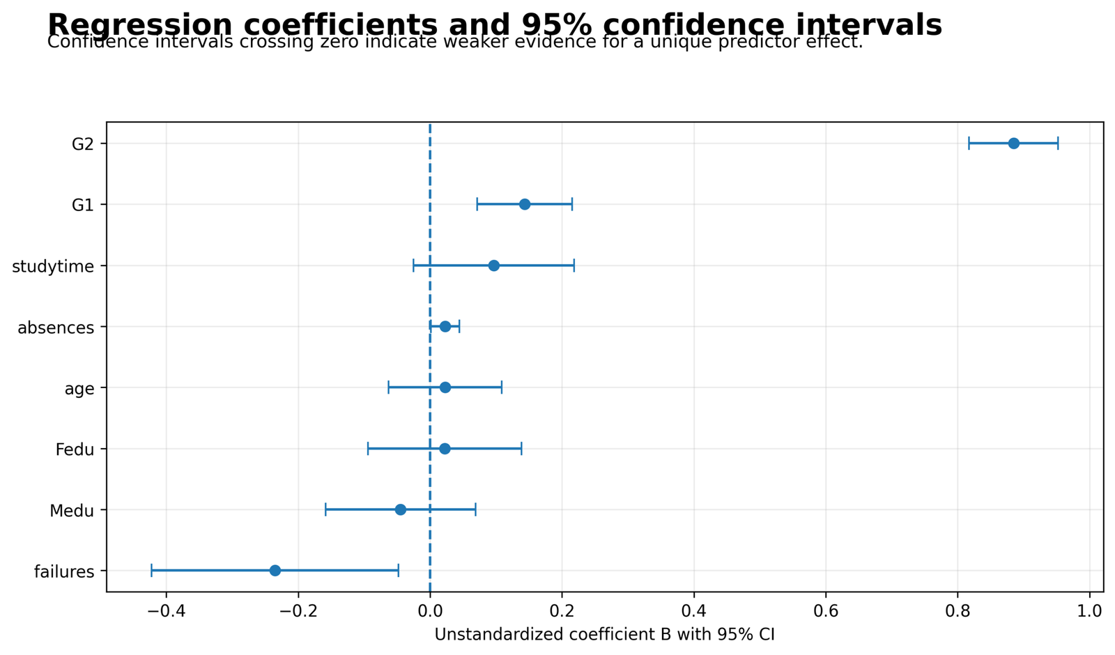
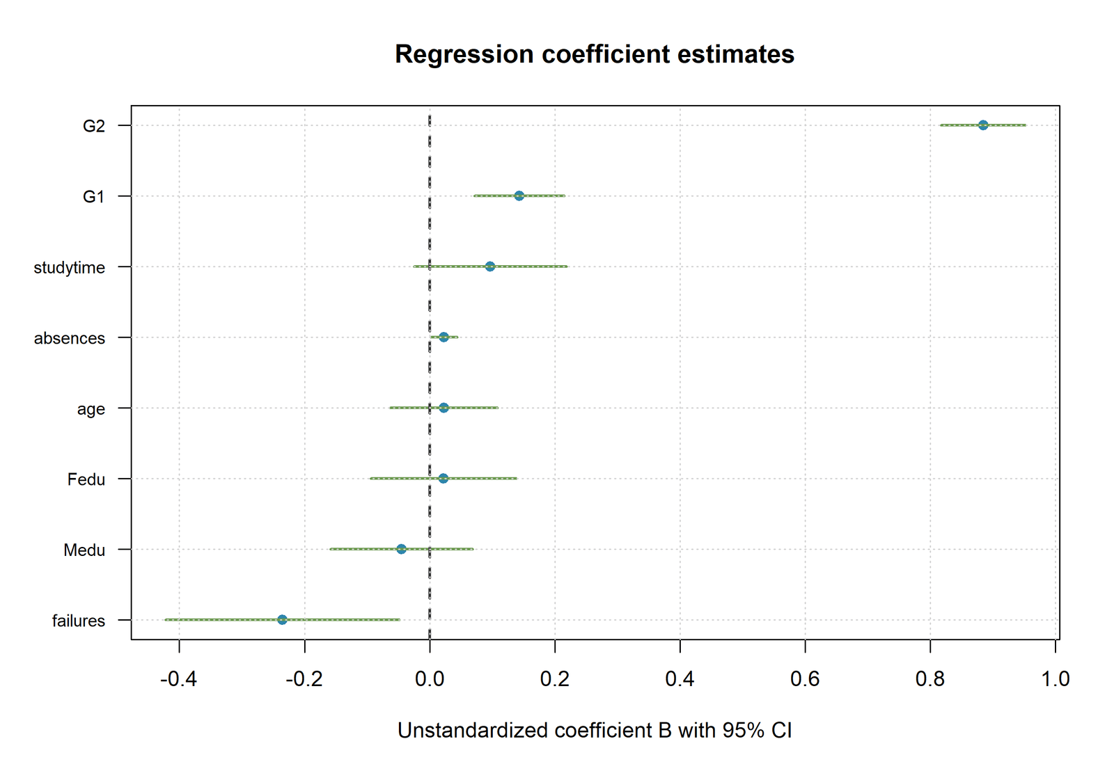
G1, G2, failures and absences remain entirely on one side of zero. The remaining predictor intervals cross zero.
G2 spans 0.817317 to 0.952298. failures spans −0.422371 to −0.048351. absences spans 0.001320 to 0.044204.
A two-sided Regression P Value below .05 and a matching 95% interval excluding zero are equivalent under the same standard error and degrees of freedom.
Confirm that each interval and probability comes from the same coefficient table and covariance estimator.
Python Chart 2: Standardized Effects
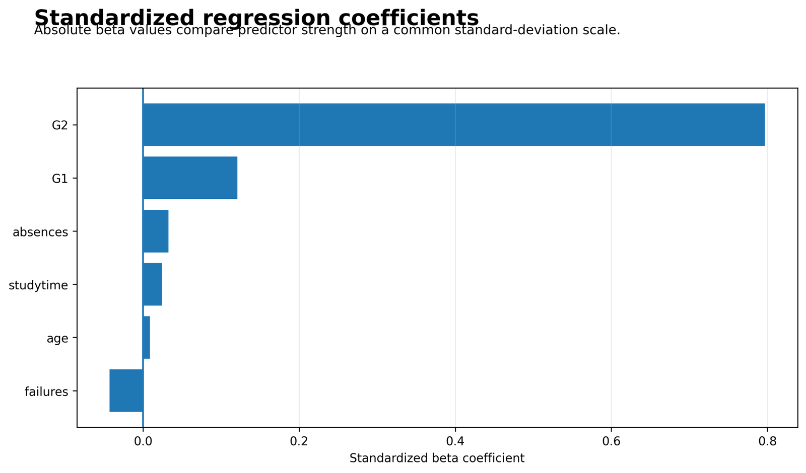
G2 dominates, G1 is a distant second and all remaining absolute standardized effects are below 0.05.
G2 β = 0.797983, G1 β = 0.121852, failures β = −0.043219 and absences β = 0.032697.
Probability evidence and effect magnitude are different. failures and absences cross .05 but have small standardized effects.
Use standard deviations from the exact 649-row model frame and retain B for original-unit interpretation.
Python Chart 3: Residuals Versus Fitted Values
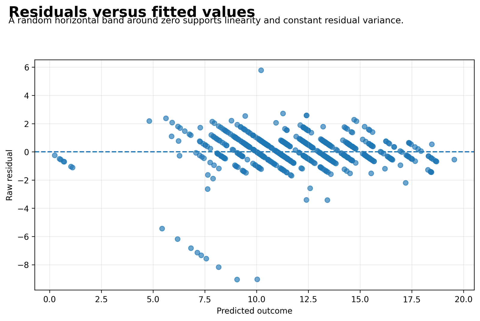
The residual cloud is broadly centered, but integer outcome bands and unusually large negative residuals remain visible.
Case 164 has predicted G3 = 9.050797, residual = −9.050797, standardized residual = −7.296333 and Cook’s distance = 0.146811.
Model form and residual variance affect the standard errors used to calculate each Regression P Value.
Review source validity, influence sensitivity and a heteroscedasticity-robust covariance table.
Python Chart 4: Association and Unique Contribution
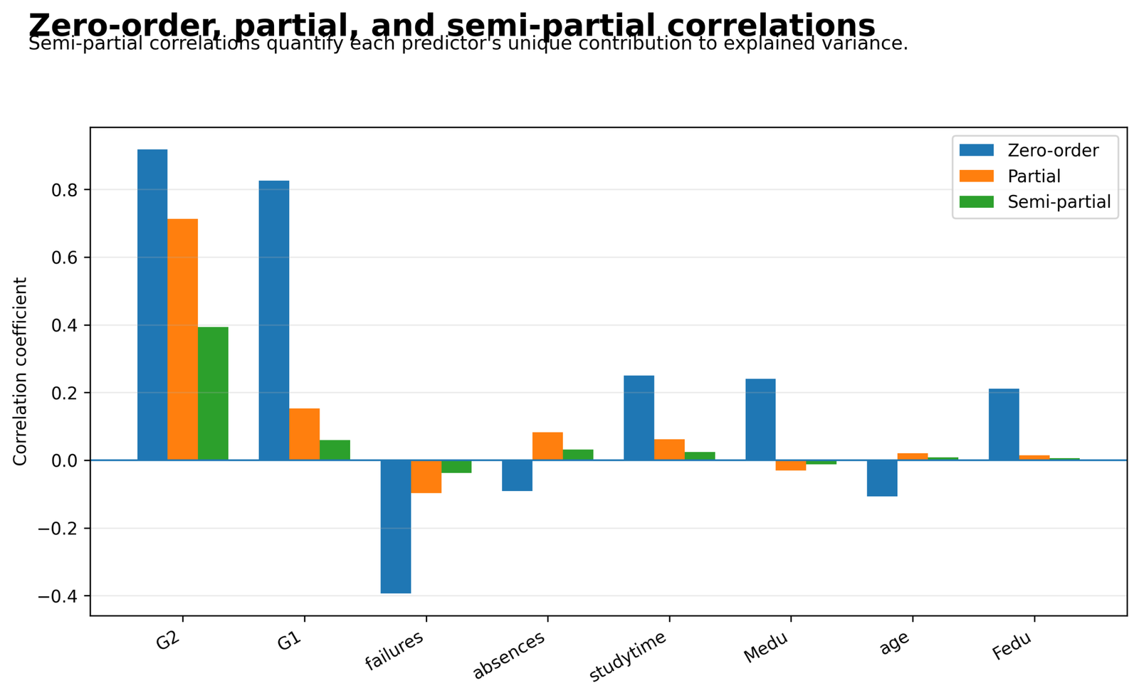
G2 remains dominant after adjustment. Several predictors have visible raw relationships but very small unique fitted contributions.
Unique R² is 0.154528 for G2, 0.003565 for G1, 0.001424 for failures and 0.001013 for absences.
A Regression P Value is not the percentage of variance uniquely explained. Equal threshold decisions can accompany very different contribution sizes.
Square each part correlation and reconcile it with the unique R² column.
R Charts and Paired Explanations
The R visuals reproduce the same Regression P Value evidence and are paired with one dedicated explanation behind each graph on desktop and mobile layouts.

Coefficient Intervals
G1, G2, failures and absences exclude zero. The absences lower limit of 0.001320 shows how close that decision is to the conventional boundary, while G2 remains far from zero across its entire interval.
confint(fit) with summary(fit)$coefficients and preserve the same 649-row model frame.Standardized Effects
G2 β = 0.797983 and G1 β = 0.121852. The remaining absolute values are small, demonstrating that crossing .05 does not automatically indicate a large standardized association.

Coefficient Probability Ranking
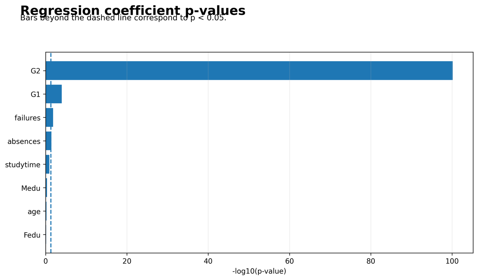
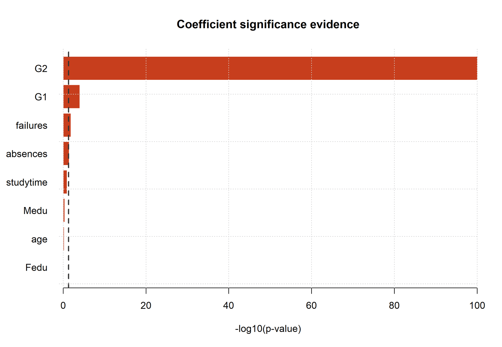
The chart separates G2 and G1 from the weaker evidence for failures and absences. studytime, age, Medu, Fedu and the intercept remain above .05.
Observed Versus Fitted
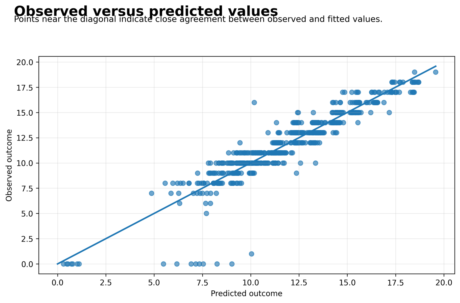
R² = 0.850777 describes strong fitted agreement, while individual vertical errors remain. The global Regression P Value concerns collective slope evidence and is not a count of correct predictions.
fitted(fit) against the response from model.frame(fit) and confirm 649 paired observations.Regression P Value Coefficient Interpretation
The coefficient table combines the original-unit estimate, confidence interval, standardized effect and unique contribution so the Regression P Value never appears without magnitude context.
| Term | B | Probability | 95% CI | Beta | Unique R² | Interpretation |
|---|---|---|---|---|---|---|
| G1 | 0.143397 | 0.000102 | [0.071385, 0.215408] | 0.121852 | 0.003565 | Strong evidence, but much smaller adjusted magnitude than G2. |
| G2 | 0.884807 | 7.355488 × 10−101 | [0.817317, 0.952298] | 0.797983 | 0.154528 | Dominant conditional predictor and unique fitted contributor. |
| studytime | 0.096632 | 0.120131 | [−0.025294, 0.218558] | 0.024811 | 0.000565 | Small positive estimate with an interval crossing zero. |
| failures | −0.235361 | 0.013718 | [−0.422371, −0.048351] | −0.043219 | 0.001424 | Negative conditional association with a small unique increment. |
| absences | 0.022762 | 0.037504 | [0.001320, 0.044204] | 0.032697 | 0.001013 | Small adjusted positive slope; not a causal benefit of absence. |
| age | 0.022685 | 0.603591 | [−0.063064, 0.108435] | 0.008554 | 0.000063 | Estimate is imprecise and close to zero on the standardized scale. |
| Medu | −0.044951 | 0.438122 | [−0.158722, 0.068820] | −0.015786 | 0.000140 | Small fitted association with considerable uncertainty. |
| Fedu | 0.022025 | 0.710518 | [−0.094451, 0.138502] | 0.007499 | 0.000032 | Smallest unique contribution in the fitted predictor set. |
G2 has both extremely strong evidence and substantial adjusted magnitude. G1 also has strong evidence, but its unique R² is only 0.003565. failures and absences demonstrate why a below-.05 result does not automatically indicate practical importance.
Predictions, Effects and Case Sensitivity
Regression P Value evidence belongs to coefficients and model comparisons, not to individual cases. Predictions, residuals, leverage and Cook’s distance are used to evaluate whether unusual observations materially affect those coefficient tests.
Fitted Equation
Case 164 Sensitivity Anchor
Case 164 has observed G3 = 0 and predicted G3 = 9.050797. Its raw residual is −9.050797, standardized residual is −7.296333, leverage is 0.024218 and Cook’s distance is 0.146811. It is unusual mainly because its outcome is far below the fitted value.
Complete Case-Level Evidence
The full 649-row prediction, residual, standardized-residual, leverage and Cook’s-distance table is preserved as a CSV inside the downloadable rewrite ZIP. It is intentionally not printed as hundreds of HTML rows because the attached sample format keeps the public post readable.
Prediction and Significance Are Different
The global model probability tests collective slope evidence. It does not measure future prediction error. Fitted RMSE = 1.247020 is calculated on the same observations used to estimate the model. External validation or correctly designed resampling is required before claiming future performance.
Regression P Value Assumptions and Diagnostics
Regression P Value calibration depends on the model, standard-error estimator and study design. A mathematically tiny value can still support a poor scientific conclusion when the equation or dependence structure is wrong.
1. Correct outcome model and linear conditional mean
G3 is treated as a continuous outcome. The expected value should be adequately represented by the stated additive linear equation. Curvature, omitted interactions or a bounded-outcome problem can change coefficient and standard-error behavior.
2. Independent observations
Independence comes from sampling and design. Repeated students, classroom clustering or ordered dependence require a covariance or multilevel structure that ordinary independent-case standard errors do not represent.
3. Suitable residual variance model
Conventional OLS uncertainty assumes a variance structure compatible with homoscedastic errors. A residual fan or changing spread supports a heteroscedasticity-robust sensitivity table rather than silent reliance on classical SE values.
4. Residual-tail and influence review
Extreme residuals can affect the estimated error variance and borderline decisions. Case 164 requires source review and coefficient sensitivity analysis.
5. No exact predictor dependence
G1 and G2 VIF values near four indicate substantial overlap. Collinearity can enlarge standard errors and make term evidence sensitive to the adjustment set, even when the overall model remains highly significant.
6. Prespecified tests and multiplicity
Testing many outcomes, interactions, subgroups or model variants increases the chance of small values under null conditions. Distinguish planned confirmation from exploration and state any adjustment method.
7. Correct missing-data and coding rules
Changing complete-case rows, factor treatment or reference categories changes estimates, SE values and probabilities. Cross-software agreement requires the same analysis frame and model matrix.
Classical Versus Robust Standard Errors
A heteroscedasticity-robust covariance estimate can leave B unchanged while changing SE, t, confidence intervals and the Regression P Value. Report the estimator, such as HC3, and keep the classical table as a separately labeled baseline. Robust SE does not repair an incorrect mean function, dependence or omitted confounding.
Influence Sensitivity
Refit the model after excluding only validated errors or as a disclosed sensitivity analysis. Compare the four borderline or moderate rows—G1, failures, absences and studytime—rather than focusing only on G2, whose evidence is unlikely to depend on small numerical changes.
Confidence-Interval Cross-Check
Every two-sided conventional coefficient result should reconcile with its 95% interval. This simple check detects mixed models, robust-versus-classical table combinations, copied columns and premature rounding.
Multiplicity and Research Families
The relevant family is defined by the scientific plan, not merely by the rows visible in one table. Eight planned predictor slopes suggest one family of eight. A larger project containing multiple outcomes, interactions and subgroup models requires a broader multiplicity discussion.
Equivalence and Minimum Important Effects
A probability above .05 does not establish equivalence. Equivalence requires a prespecified interval of effects considered practically negligible and a procedure such as two one-sided tests. The question “is the coefficient exactly zero?” differs from “is the coefficient small enough to ignore?”
Regression P Value in Python, R, SPSS and Excel
Regression P Value values should agree across software when the rows, model matrix, estimator, degrees of freedom and standard-error method are identical.
Python
statsmodels returns B, SE, t, term probabilities, intervals, F, global probability, AIC, BIC and case influence from one OLS object.
- Use one complete-case DataFrame.
- Add the intercept explicitly.
- Retain full precision in CSV files.
- Label fitted RMSE and residual SE separately.
R
lm() and summary.lm() provide coefficient and global evidence. confint(), model.frame() and influence methods preserve the object audit trail.
- Confirm 649 model-frame rows.
- Inspect variable classes.
- Use the same formula in all exports.
- Save session information.
SPSS
The Coefficients table reports B, SE, Beta, t, Sig. and intervals. The ANOVA table reports the separate global F probability.
- Use METHOD=ENTER.
- Report Sig. .000 as p < .001.
- Request collinearity and casewise output.
- Save predicted and diagnostic variables.
Excel
The workbook reproduces the tail calculation from full-precision B and SE values using 640 degrees of freedom.
- Use T.DIST.2T for term tests.
- Use F.DIST.RT for the global test.
- Avoid rounding before calculation.
- Check intervals and decisions together.
Code: Expand Only the Software You Need
Each panel calculates or audits Regression P Value evidence for the same eight-predictor specification.
Python Regression P Value workflow
from pathlib import Path
import numpy as np
import pandas as pd
import statsmodels.api as sm
from scipy import stats
from statsmodels.stats.outliers_influence import variance_inflation_factor

DATA = Path("dataset.csv")
OUTCOME = "G3"
PREDICTORS = [
    "G1", "G2", "studytime", "failures",
    "absences", "age", "Medu", "Fedu"
]

raw = pd.read_csv(DATA)
model_data = raw[[OUTCOME] + PREDICTORS].dropna().copy()

y = model_data[OUTCOME].astype(float)
X = sm.add_constant(model_data[PREDICTORS].astype(float), has_constant="add")
fit = sm.OLS(y, X).fit()

ci = fit.conf_int(alpha=0.05)
coef_table = pd.DataFrame({
    "term": fit.params.index,
    "B": fit.params.values,
    "SE": fit.bse.values,
    "t": fit.tvalues.values,
    "p_value": fit.pvalues.values,
    "CI95_lower": ci[0].values,
    "CI95_upper": ci[1].values,
})

# Standardized beta for numeric slopes.
y_sd = y.std(ddof=1)
beta = fit.params[PREDICTORS] * model_data[PREDICTORS].std(ddof=1) / y_sd
standardized = pd.DataFrame({
    "term": PREDICTORS,
    "B": fit.params[PREDICTORS].values,
    "standardized_beta": beta.values,
})

# VIF excludes the intercept from substantive interpretation.
vif = pd.DataFrame({
    "term": PREDICTORS,
    "VIF": [
        variance_inflation_factor(
            model_data[PREDICTORS].astype(float).to_numpy(), i
        )
        for i in range(len(PREDICTORS))
    ],
})
vif["tolerance"] = 1 / vif["VIF"]

influence = fit.get_influence()
case_audit = model_data.copy()
case_audit["predicted_value"] = fit.fittedvalues
case_audit["raw_residual"] = fit.resid
case_audit["standardized_residual"] = influence.resid_studentized_internal
case_audit["studentized_residual"] = influence.resid_studentized_external
case_audit["leverage"] = influence.hat_matrix_diag
case_audit["cooks_distance"] = influence.cooks_distance[0]

model_summary = pd.DataFrame([{
    "n": int(fit.nobs),
    "df_model": float(fit.df_model),
    "df_residual": float(fit.df_resid),
    "r_squared": fit.rsquared,
    "adjusted_r_squared": fit.rsquared_adj,
    "f_statistic": fit.fvalue,
    "f_p_value": fit.f_pvalue,
    "fitted_rmse": np.sqrt(np.mean(fit.resid ** 2)),
    "residual_standard_error": np.sqrt(fit.ssr / fit.df_resid),
    "aic": fit.aic,
    "bic": fit.bic,
}])

coef_table.to_csv("regression_p_value_coefficients.csv", index=False)
standardized.to_csv("regression_p_value_standardized_betas.csv", index=False)
vif.to_csv("regression_p_value_vif.csv", index=False)
case_audit.to_csv("regression_p_value_case_audit.csv", index=False)
model_summary.to_csv("regression_p_value_model_summary.csv", index=False)

print(model_summary.to_string(index=False))
print(coef_table.to_string(index=False))
R Regression P Value workflow
dat <- read.csv("dataset.csv", check.names = FALSE)

outcome <- "G3"
predictors <- c(
  "G1", "G2", "studytime", "failures",
  "absences", "age", "Medu", "Fedu"
)

model_dat <- dat[complete.cases(dat[c(outcome, predictors)]),
                 c(outcome, predictors)]

fit <- lm(
  G3 ~ G1 + G2 + studytime + failures +
    absences + age + Medu + Fedu,
  data = model_dat
)

s <- summary(fit)
ci <- confint(fit, level = 0.95)
coef_matrix <- s$coefficients

coef_table <- data.frame(
  term = rownames(coef_matrix),
  B = coef_matrix[, 1],
  SE = coef_matrix[, 2],
  t_value = coef_matrix[, 3],
  p_value = coef_matrix[, 4],
  CI95_lower = ci[, 1],
  CI95_upper = ci[, 2],
  row.names = NULL
)

# Standardized beta for the numeric predictor set.
response_sd <- sd(model_dat[[outcome]])
beta <- coef(fit)[predictors] *
  vapply(model_dat[predictors], sd, numeric(1)) / response_sd

standardized <- data.frame(
  term = predictors,
  B = coef(fit)[predictors],
  standardized_beta = unname(beta),
  row.names = NULL
)

# Case-level audit.
case_audit <- transform(
  model.frame(fit),
  predicted_value = fitted(fit),
  raw_residual = residuals(fit),
  standardized_residual = rstandard(fit),
  studentized_residual = rstudent(fit),
  leverage = hatvalues(fit),
  cooks_distance = cooks.distance(fit)
)

model_summary <- data.frame(
  n = nobs(fit),
  df_model = unname(s$fstatistic[2]),
  df_residual = unname(s$fstatistic[3]),
  r_squared = s$r.squared,
  adjusted_r_squared = s$adj.r.squared,
  f_statistic = unname(s$fstatistic[1]),
  f_p_value = pf(
    unname(s$fstatistic[1]),
    unname(s$fstatistic[2]),
    unname(s$fstatistic[3]),
    lower.tail = FALSE
  ),
  fitted_rmse = sqrt(mean(residuals(fit)^2)),
  residual_standard_error = s$sigma,
  aic = AIC(fit),
  bic = BIC(fit)
)

write.csv(coef_table, "regression_p_value_coefficients.csv",
          row.names = FALSE)
write.csv(standardized, "regression_p_value_standardized_betas.csv",
          row.names = FALSE)
write.csv(case_audit, "regression_p_value_case_audit.csv",
          row.names = FALSE)
write.csv(model_summary, "regression_p_value_model_summary.csv",
          row.names = FALSE)

print(model_summary)
print(coef_table)
SPSS Regression P Value syntax
* Regression P Value: eight-predictor linear regression.

REGRESSION
 /MISSING LISTWISE
 /STATISTICS COEFF OUTS R ANOVA CHANGE CI(95) COLLIN TOL ZPP
 /CRITERIA=PIN(.05) POUT(.10) TOLERANCE(.0001)
 /NOORIGIN
 /DEPENDENT G3
 /METHOD=ENTER G1 G2 studytime failures absences age Medu Fedu
 /RESIDUALS DURBIN
 /CASEWISE PLOT(ZRESID) OUTLIERS(3)
 /SAVE
  PRED(rpv_pred)
  RESID(rpv_resid)
  ZPRED(rpv_zpred)
  ZRESID(rpv_zresid)
  SRESID(rpv_sresid)
  MAHAL(rpv_mahal)
  COOK(rpv_cook)
  LEVER(rpv_lev).

* SPSS displays very small probabilities as .000.
* Report them as p < .001 rather than p = 0.

DESCRIPTIVES VARIABLES=
 rpv_pred rpv_resid rpv_zpred rpv_zresid
 rpv_sresid rpv_mahal rpv_cook rpv_lev
 /STATISTICS=MEAN STDDEV MIN MAX.

GRAPH
 /SCATTERPLOT(BIVAR)=rpv_pred WITH G3
 /TITLE='Observed and Predicted G3'.

GRAPH
 /SCATTERPLOT(BIVAR)=rpv_pred WITH rpv_resid
 /TITLE='Residuals and Predicted Values'.

GRAPH
 /HISTOGRAM(NORMAL)=rpv_resid
 /TITLE='Residual Distribution'.
Excel Regression P Value formulas
Assume:
B2 = coefficient B
C2 = coefficient standard error
D2 = residual degrees of freedom, 640
E2 = significance level, 0.05

t statistic
=B2/C2

two-sided coefficient probability
=T.DIST.2T(ABS(B2/C2),D2)

95% critical t
=T.INV.2T(E2,D2)

95% confidence lower limit
=B2-T.INV.2T(E2,D2)*C2

95% confidence upper limit
=B2+T.INV.2T(E2,D2)*C2

interval decision
=IF(AND(LowerCell<=0,UpperCell>=0),
   "Interval includes zero",
   "Interval excludes zero")

global F probability
=F.DIST.RT(FStatisticCell,8,640)

Bonferroni reference for eight planned predictor tests
=0.05/8

Bonferroni reference for all nine displayed coefficient rows
=0.05/9
Advanced Regression P Value Topics
Regression P Value evidence changes meaning when multiplicity, robust covariance, categorical terms, model selection or equivalence questions are introduced.
Global significance versus term significance
The global F test can be extremely small because one or two predictors carry strong signal. It does not imply that every coefficient row crosses .05.
Robust standard errors
HC3 or another heteroscedasticity-robust covariance estimator leaves the OLS B values unchanged but can alter SE, t, intervals and the Regression P Value. Label the robust table separately.
Categorical predictors
A factor with several levels produces several indicator coefficients. The scientific question about the factor as a whole normally requires a multi-degree-of-freedom joint test rather than interpreting one reference-category row alone.
Model selection and post-selection inference
Trying many transformations, interactions or stepwise models and reporting only the final ordinary probability makes that table optimistic. Treat it as exploratory or use a procedure designed for the selection process.
Equivalence testing
A value above .05 does not establish a negligible effect. Define a smallest effect of interest and test whether the complete interval lies inside the equivalence region.
Prediction versus inference
A predictor can help external prediction even when its individual coefficient test is uncertain. Conversely, a tiny Regression P Value does not guarantee useful new-case accuracy.
Multiplicity Sensitivity
| Rule | Reference threshold | Predictors remaining below the threshold | Meaning |
|---|---|---|---|
| Unadjusted eight-predictor family | 0.05000 | G1, G2, failures, absences | Conventional individual coefficient decisions. |
| Bonferroni for eight planned slopes | 0.00625 | G1 and G2 | Conservative familywise-error sensitivity. |
| Bonferroni for nine displayed rows | 0.00556 | G1 and G2 | Includes the intercept, which is often outside the scientific family. |
| Holm procedure | Stepwise thresholds | Depends on ordered exact values | Controls familywise error and is usually less conservative than Bonferroni. |
The correct multiplicity family comes from the research plan. It may include several outcomes, interactions and subgroup models rather than only the eight slopes shown here.
- Regression P Value should always be tied to a stated null.
- Regression P Value should be reported with B, SE and a confidence interval.
- Regression P Value should not replace standardized or practical effect evidence.
- Regression P Value should use the correct residual degrees of freedom.
- Regression P Value should be recalculated after changing the covariance estimator.
- Regression P Value should be interpreted within the declared multiplicity family.
- Regression P Value should remain separate from prediction accuracy.
- Regression P Value should not justify causal language by itself.
APA-Style Reporting
Regression P Value reporting should identify the model, sample, coefficient scale, uncertainty method and diagnostics rather than listing isolated probability values.
For exact scientific reporting, use the full probability for G2 in a table or write p < .001 in prose. State whether classical or robust standard errors support the conclusion and disclose any multiplicity or influence sensitivity analysis.
Publication Checklist
- Use the exact focus phrase Regression P Value naturally throughout the post.
- State the outcome, all eight predictors and N = 649.
- State 640 residual degrees of freedom.
- Separate coefficient, global and block probability tests.
- Report B, SE, t, probability and 95% interval.
- Report R² and adjusted R² as magnitude, not probability.
- Label fitted RMSE and residual standard error correctly.
- Report standardized Beta and unique R² separately.
- Exclude intercept VIF from substantive collinearity interpretation.
- Explain the G1 and G2 overlap.
- Interpret the absences sign change cautiously.
- Do not treat nonsignificance as equivalence.
- State the multiplicity family and any adjustment.
- Review residuals, leverage, Cook’s distance and case 164.
- Verify all 12 chart URLs and captions.
- Verify the four software download links.
- Retain all advertisement placements and the back-to-top control.
Downloads and Chart Resources
The Regression P Value evidence package contains Python, R, SPSS and Excel results plus the 12 supplied charts.
R reportSame-model cross-software verification
SPSS outputModel Summary, ANOVA, Coefficients and diagnostics
Worked Excel workbookFull-precision t, F, interval and decision formulas
Python chart 1Coefficient intervals
Python chart 2Standardized effects
Python chart 3Minus-log probability ranking
Python chart 4Observed versus predicted
Python chart 5Residuals versus fitted
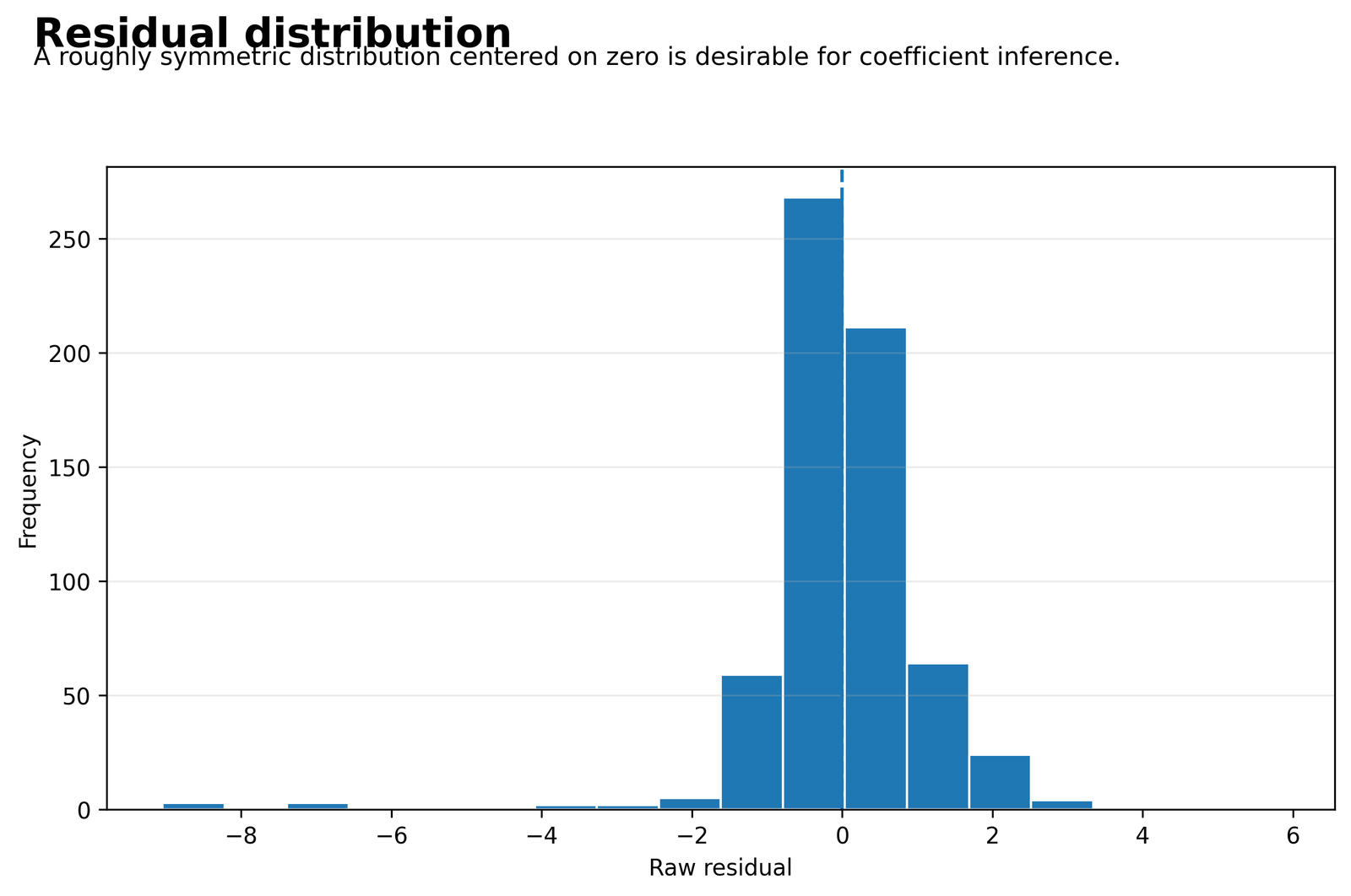
Python chart 6Residual distribution
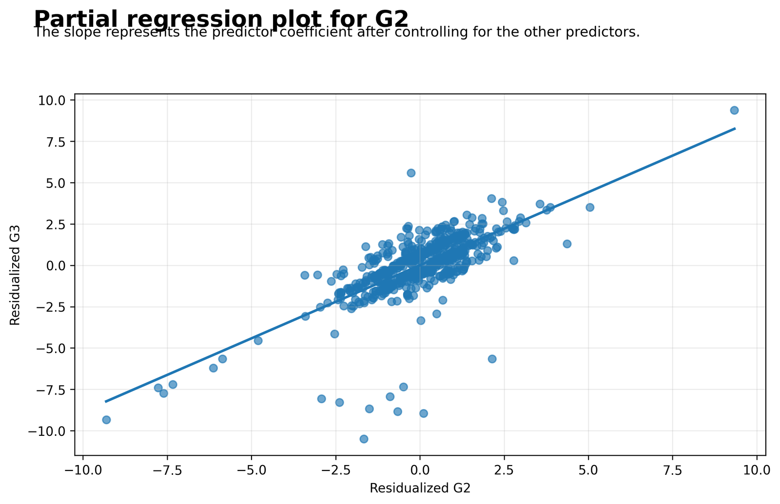
Python chart 7Partial G2 relationship
Python chart 8Association and unique contribution
R chart 1Coefficient intervals
R chart 2Standardized effects
R chart 3Coefficient probability ranking
R chart 4Observed versus fitted
Frequently Asked Questions
What null hypothesis does each coefficient test?
Each slope tests H₀: βj = 0 after controlling for the other seven predictors in the same equation.
What does the global Regression P Value test?
It tests whether all eight non-intercept slopes equal zero together. It does not say that every separate predictor is significant.
Is the Regression P Value the probability that the null is true?
No. It is a tail probability calculated under the null and model assumptions. It does not assign a posterior probability to the null hypothesis.
Why is G2’s value so small?
Its coefficient is large relative to its standard error: 0.884807 / 0.034369 = 25.743971. It also has a large standardized Beta and unique fitted contribution.
Does p = .037504 for absences prove an effect?
It crosses the unadjusted .05 rule under the conventional model, but the coefficient is small, the interval begins near zero, multiplicity matters and the adjusted sign differs from the zero-order relationship.
Does p above .05 prove no association?
No. The interval shows the range of effects compatible with the data and model. A separate equivalence design is required to support a negligible-effect claim.
Why report confidence intervals?
They show direction, precision and compatible effect values. A threshold alone hides whether the estimate is large, small or uncertain.
Why report standardized Beta?
Beta compares fitted slopes in standard-deviation units. It adds magnitude context but remains sample dependent and noncausal.
What is unique R²?
It is the squared part correlation for a predictor and represents the fitted R² increment uniquely associated with that predictor after the others are retained.
Why is the fitted RMSE different from 1.255758?
Fitted RMSE uses N in the denominator and is about 1.247020. The value 1.255758 is residual standard error using 640 residual degrees of freedom.
Should the intercept be included in multiplicity correction?
Usually the scientific family concerns predictor slopes, not the intercept. State the planned family rather than automatically counting every displayed row.
What happens under Bonferroni correction?
For eight predictor slopes, the reference is .00625. G1 and G2 remain below it; failures and absences do not. This is a sensitivity result unless Bonferroni was prespecified.
Can robust standard errors change the conclusion?
Yes. They leave OLS B values unchanged but can alter SE, t, confidence intervals and the Regression P Value.
Should case 164 be deleted?
No automatic deletion is justified. Verify the source record and report sensitivity results. A difficult-to-predict valid case may belong to the target population.
How does Excel reproduce a coefficient result?
Calculate B/SE, take the absolute value and use T.DIST.2T with 640 degrees of freedom. Use full-precision inputs.
Why does SPSS show Sig. .000?
The displayed probability is smaller than the table precision. Report p < .001, not p = 0.
Can a significant model predict poorly?
Yes. Significance concerns evidence against a null. Prediction concerns error and generalization. A large sample can yield strong evidence for a model with limited predictive value.
Can a useful predictor have p above .05?
Yes, especially in prediction, under collinearity or when the sample provides limited precision. Model purpose and external validation matter.
Regression P Value Conclusion
Regression P Value evidence for the verified eight-predictor model is collectively decisive, F(8, 640) = 456.111097, probability = 1.454898 × 10−258. The strongest term evidence belongs to G2, followed by G1. failures and absences cross the conventional .05 threshold but have small standardized and unique fitted contributions.
studytime, age, Medu and Fedu remain uncertain under the conventional model. Their results do not prove exact zero. The coefficient intervals, multiplicity family, residual behavior, G1-G2 overlap and case 164 sensitivity all qualify the final interpretation.
The correct reporting strategy is to connect every Regression P Value with its null, estimate, standard error, degrees of freedom, confidence interval, effect magnitude, unique contribution and diagnostic context. This prevents a threshold from becoming the entire scientific conclusion.