
Regression in Excel: Formulas, Data Analysis ToolPak, LINEST, Interpretation and Worked Workbook
Regression in Excel can be transparent, reproducible and statistically useful when the data ranges, model formula, coefficient order, prediction cells and diagnostic calculations are all controlled. This Excel-only guide follows 649 complete observations through a simple regression, an eight-predictor multiple regression, worksheet predictions, residual checks, standardized coefficients, workbook protection and reporting.
1 simple predictor
8 multiple predictors
9-sheet Excel workflow
Regression in Excel Model Overview
Regression in Excel is most useful when the model and the spreadsheet implementation are reviewed as one connected workflow.
Regression in Excel estimates how a continuous outcome changes with one or more predictors. The worked workbook predicts the final grade G3. The simple model uses G2 alone, while the multiple model uses G1, G2, studytime, failures, absences, age, Medu and Fedu. Both models use the same 649 complete rows, so changes in fit are attributable to model specification rather than a changing sample.
The workbook is designed as an audit trail rather than a screenshot collection. Source values feed descriptive statistics and correlations, verified coefficients feed prediction formulas, observed values are compared with fitted values, residuals are calculated row by row, and summary cells reconcile model fit, ANOVA and standardized effects. The attached workbook and report therefore support both learning and verification.
What Is Regression in Excel?
Regression in Excel can be carried out with native functions, the Data Analysis ToolPak, LINEST, or a carefully designed workbook that stores verified values and recalculates downstream formulas. The method is ordinary least squares: it chooses coefficients that minimize the sum of squared residuals, where each residual is observed G3 minus predicted G3.
The simple model answers a bivariate question: how does expected G3 change with G2? The multiple model answers a conditional question: how does expected G3 change with one predictor while the other seven listed predictors remain fixed? These are different estimands even when both are calculated in the same workbook.
When Should Regression in Excel Be Used?
Good uses
- Teaching simple and multiple linear regression with visible arithmetic.
- Building a reviewable prediction calculator from a fixed model.
- Auditing a modest dataset with controlled ranges and protected formulas.
- Reproducing coefficients, fitted values, residuals and standardized betas.
- Sharing a workbook with users who need cell-level transparency.
Weak uses
- Very large or frequently changing datasets without structured range control.
- Workflows that require extensive resampling, automation or version history.
- Situations where users may overwrite formulas or sort columns independently.
- Claims of causal effect from observational worksheet associations.
- Claims of future accuracy based only on fitted-sample RMSE.
Core Regression in Excel Formulas
Regression in Excel Assumptions and Requirements
1. Continuous outcome and correct equation
The standard worksheet predicts a continuous outcome. G3 is treated as continuous. A binary, count, ordinal or time-to-event outcome requires a different model rather than the same linear formulas.
2. One aligned analysis frame
Outcome and predictor ranges must refer to the same rows in the same order. Removing a blank from only one column can silently pair one student’s outcome with another student’s predictors.
3. Linear conditional mean
The fitted equation assumes that expected G3 is adequately represented by a linear combination of the selected predictors. Residual patterns should be checked for curvature.
4. Independent observations
Rows should represent independent observational units. A spreadsheet formula cannot establish independence; that requirement comes from the study design.
5. Stable residual variance
Classical standard errors and confidence intervals assume reasonably constant residual spread across fitted values. A residual-versus-fitted chart is an important check.
6. No perfect multicollinearity
Predictor columns cannot be exact linear combinations. G1 and G2 overlap strongly, so VIF and tolerance should be reviewed rather than ignored.
7. Protected formulas and automatic recalculation
Input cells should be clearly marked, calculation cells should be protected, and Excel should be in automatic calculation mode before results are distributed.
Current Worked Scenario
The verified workbook uses rows 4 through 652 on the Data sheet, giving 649 observations. The simple equation predicts G3 from G2. The multiple equation includes eight predictors. The workbook records a simple-model R² of 0.843730 and a multiple-model R² of 0.850777. The richer equation therefore improves fitted description modestly because G2 already contains most of the available predictive signal.
Quick Answer
Regression in Excel gives the strongest answer when model fit, coefficient uncertainty and workbook integrity are reported together.
What the Excel output supports
- 649 complete observations are included in both fitted models.
- The eight-predictor equation explains 85.08% of fitted G3 variation.
- The complete predictor block is statistically significant, F = 456.111097.
- G2 is the dominant conditional predictor in standardized units.
- G1, G2, failures and absences have 95% intervals excluding zero.
What the Excel output does not prove
- It does not establish that changing a predictor causes G3 to change.
- It does not prove that every included predictor is practically important.
- It does not guarantee an RMSE of 1.247020 on future observations.
- It does not make a broken range, overwritten formula or wrong column order harmless.
- It does not replace residual, collinearity and influence review.
Table of Contents
Regression in Excel is organized below from data control and estimation through diagnostics, reporting and download verification.
- Why this analysis needs Regression in Excel
- How Regression in Excel works
- Workbook structure and sheet roles
- Variables, ranges and coding
- Regression in Excel results
- Excel workbook charts and explanations
- Coefficient interpretation
- Predictions and worksheet calculations
- Assumptions and diagnostics
- Excel procedures and reproducibility
- Excel formulas and LINEST
- Advanced Regression in Excel topics
- APA-style reporting
- Publication checklist
- Downloads and chart resources
- Related Salar Cafe guides
- Frequently asked questions
- Regression in Excel conclusion
Why This Analysis Needs Regression in Excel
Regression in Excel is appropriate here because the simple and multiple equations can be traced from source rows to final residuals.
The analytical question has two levels. The simple worksheet asks how G3 changes with G2 alone. The multiple worksheet asks how G3 changes with each predictor after adjustment for the other seven variables. Regression in Excel is useful here because the workbook makes that distinction visible through separate sheets, equations and residual columns.
The README identifies G3 as the outcome, G2 as the simple predictor, and G1, G2, studytime, failures, absences, age, Medu and Fedu as the multiple predictor block. Both models use 649 rows. Keeping the sample fixed prevents a misleading comparison caused by different missing-data patterns.
Why the simple model matters
- Demonstrates SLOPE, INTERCEPT, CORREL, RSQ and STEYX.
- Provides a clear one-variable equation.
- Shows how closely G2 alone tracks G3.
- Creates a benchmark for the multiple model.
Why the multiple model matters
- Separates conditional from zero-order associations.
- Quantifies the incremental contribution of G1 beyond G2.
- Shows why signs may change after adjustment.
- Supports a richer prediction calculator and residual audit.
A spreadsheet is not automatically transparent merely because cells are visible. Transparency requires consistent ranges, labeled coefficients, preserved formulas, documented assumptions, and verification that charts point to live diagnostic columns rather than copied static values.
How Regression in Excel Works
Regression in Excel works reliably only when every calculation stage uses the same eligible observations and declared predictor order.
Keep G3 and all predictors aligned across the same 649 eligible rows.
Use native functions, LINEST or the Analysis ToolPak with declared ranges.
Reconcile predictions, residuals, ANOVA, intervals, charts and dashboard cells.
Simple Regression in Excel
The simple worksheet uses G3 as known y and G2 as known x. The verified slope is 1.018490 and the verified intercept is 0.121966. A one-point increase in G2 is associated with an expected 1.018490-point increase in G3 in the simple fitted equation.
Multiple Regression in Excel
The multiple equation contains eight slopes plus an intercept. A prediction row must multiply each input by the coefficient carrying the same label. A correct numerical formula with a wrong column order is still a wrong model. This is especially important when LINEST is used because its coefficient array is returned in reverse order relative to the known x columns.
The verified equation is stored explicitly so the Diagnostics sheet can calculate each fitted value. The row residual is then observed G3 minus fitted G3. Squared residuals feed RMSE and the residual sum of squares; absolute residuals feed MAE-style summaries.
Analysis ToolPak Procedure
- Arrange G3 and all predictors in aligned columns with clear labels.
- Open Data → Data Analysis → Regression.
- Select the complete G3 range as the Input Y Range.
- Select the complete predictor block as the Input X Range.
- Check Labels only when the selected ranges include headers.
- Keep the intercept unless the research model genuinely requires a zero intercept.
- Select a 95% confidence level and request residual output.
- Record the exact input ranges and output-sheet location.
- Reconcile the ToolPak coefficients with the labeled workbook equation.
Residual Plot and Formula Consistency
The residual-versus-fitted chart uses residual = observed G3 − predicted G3. A centered cloud is desirable. Curvature suggests that the linear mean is incomplete, while changing vertical spread suggests nonconstant variance. Integer-valued grades can create visible diagonal bands even when the formula is correct.
Sort only a copy when reviewing large residuals. Sorting one column independently can destroy row alignment, and filtering can make an apparently complete chart omit cases. A stable diagnostic sheet should retain case identifiers and fixed chart references.
Formula Protection and Recalculation
The workbook marks editable cells and depends on preserved formulas across nine sheets. Before distribution, leave data and prediction-input cells unlocked, protect coefficient and diagnostic cells, set calculation to automatic, force a full recalculation, save, close and reopen the file, and compare the headline values with the verified report.
Regression in Excel Workbook Structure
Regression in Excel becomes easier to audit when source data, fitted evidence, diagnostics and user inputs are separated by worksheet role.
The nine-sheet structure separates source data, calculations, interpretation and user input. This separation reduces the risk that one pasted value silently replaces a model formula.
Variables Used, Coding and Range Control
Regression in Excel requires a clear data dictionary so each cell range has one statistical meaning.
| Variable | Role | Meaning | Excel treatment |
|---|---|---|---|
| G3 | Outcome | Final course grade. | Known y range; observed value used in residual calculations. |
| G2 | Simple and multiple predictor | Second-period grade. | Known x in the simple model; included in the eight-column block. |
| G1 | Multiple predictor | First-period grade. | Numeric predictor with a conditional slope. |
| studytime | Multiple predictor | Weekly study-time category. | Treated as an ordered numeric input. |
| failures | Multiple predictor | Number of previous class failures. | Numeric count. |
| absences | Multiple predictor | School absence count. | Numeric count; sign requires conditional interpretation. |
| age | Multiple predictor | Age in years. | Numeric predictor. |
| Medu | Multiple predictor | Mother’s education level. | Ordered numeric predictor. |
| Fedu | Multiple predictor | Father’s education level. | Ordered numeric predictor. |
Data Layout and Complete-Case Control
The formulas use rows 4 through 652, which yields 649 observations. Regression in Excel should use one analysis mask across the outcome and all predictors. Pairwise descriptive correlations may use more observations when blanks differ by column, but those counts must not be confused with the listwise regression sample.
Before fitting, compare COUNT for G3 and every selected predictor. When adding new rows, extend all source, prediction, residual, chart and summary ranges together. A structured Excel table is safer than editing many fixed endpoints independently.
Standardization
The regression coefficients B remain in original units. Standardized beta is calculated after fitting:
Standardized beta supports scale comparison inside the fitted sample. It is not a causal ranking and may change in another population because both the coefficients and sample standard deviations can change.
Regression in Excel Results
Regression in Excel results should be read from the verified coefficient, ANOVA and fit blocks rather than from isolated dashboard numbers.
Complete rows used in both models
G3 predicted from G2 alone
Eight-predictor fitted proportion
Penalty for eight predictors
Fitted error on the G3 scale
Joint test of the predictor block
Verified Model Results
| Model | N | R² | Adjusted R² | F statistic | RMSE / standard error |
|---|---|---|---|---|---|
| Simple: G3 on G2 | 649 | 0.843730 | 0.843489 | 3493.281566 | 1.278096 |
| Multiple: eight predictors | 649 | 0.850777 | 0.848912 | 456.111097 | 1.247020 |
The increase in R² is 0.007047. This is a real fitted improvement, but it is modest because G2 alone already predicts G3 strongly. The multiple model is justified when the goal is a conditional equation or a richer prediction worksheet, not merely because its R² is numerically larger.
ANOVA Decomposition in Cells
| Source | Sum of squares | df | Mean square | Interpretation |
|---|---|---|---|---|
| Regression | 5754.032978 | 8 | 719.254122 | Variation attributed to the complete predictor block. |
| Residual | 1009.233586 | 640 | 1.576927 | Unexplained squared error remaining after fitting. |
| Total | 6763.266564 | 648 | — | Total corrected G3 variation. |
Regression SS plus residual SS equals total SS within displayed precision. The overall F statistic equals regression mean square divided by residual mean square: 719.254122 / 1.576927 ≈ 456.111097. These identities are powerful workbook checks because a broken range often appears first as a failure of reconciliation.
Verified Coefficient Evidence
| Term | B | SE | t | p | 95% CI | Standardized beta |
|---|---|---|---|---|---|---|
| Intercept | −0.501155 | 0.773950 | −0.6475 | 0.5175 | [−2.0209, 1.0186] | — |
| G1 | 0.143397 | 0.036672 | 3.9103 | 0.000102 | [0.0714, 0.2154] | 0.121852 |
| G2 | 0.884807 | 0.034369 | 25.7440 | 7.355e−101 | [0.8173, 0.9523] | 0.797983 |
| studytime | 0.096632 | 0.062091 | 1.5563 | 0.1201 | [−0.0253, 0.2186] | 0.024811 |
| failures | −0.235361 | 0.095234 | −2.4714 | 0.0137 | [−0.4224, −0.0484] | −0.043219 |
| absences | 0.022762 | 0.010919 | 2.0846 | 0.0375 | [0.0013, 0.0442] | 0.032697 |
| age | 0.022685 | 0.043668 | 0.5195 | 0.6036 | [−0.0631, 0.1084] | 0.008554 |
| Medu | −0.044951 | 0.057938 | −0.7759 | 0.4381 | [−0.1587, 0.0688] | −0.015786 |
| Fedu | 0.022025 | 0.059316 | 0.3713 | 0.7105 | [−0.0945, 0.1385] | 0.007499 |
Download the Excel Regression Files
Use the workbook for formulas and the verified report for the saved benchmark values.
Excel Workbook Charts and Explanations
Regression in Excel charts are useful only when their plotted series remain linked to complete live worksheet ranges.
These figures visualize calculations from the worked Regression in Excel workbook. Each chart is explained through the visible pattern, exact saved values, statistical meaning and the next cell-level check.
Excel Chart 1: Observed G3 Versus Workbook Prediction
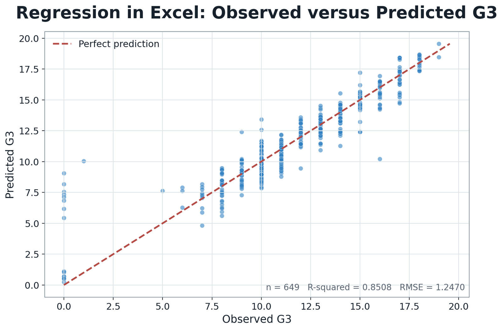
Most points follow the identity direction, showing strong agreement between observed and fitted grades across the dense central range.
The multiple worksheet reports R² = 0.850777, adjusted R² = 0.848912 and fitted RMSE = 1.247020.
The equation captures most fitted variation, but vertical distance from the identity line remains the case-level error. Extreme outcomes can still be predicted poorly.
Select several early, middle and late rows; recompute the prediction from the coefficient cells and verify that the plotted coordinates match the Diagnostics sheet.
Excel Chart 2: Workbook Residuals Versus Fitted Values
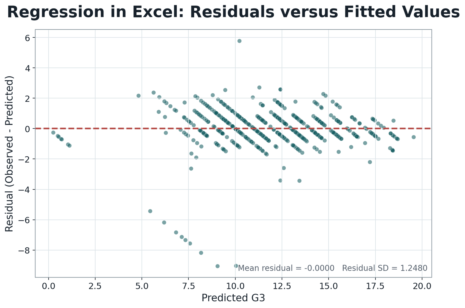
The zero reference separates underprediction from overprediction. Integer-valued grades create visible bands, while isolated large errors extend the vertical scale.
The fitted RMSE is 1.247020. The residual sum of squares is 1009.233586 across 640 residual degrees of freedom.
Curvature would question the linear mean function; widening spread would question constant variance. A centered cloud alone does not establish normality or independence.
Sort a copied diagnostic table by absolute residual, retain the original case identifier, and verify that chart ranges still point to the unsorted full table.
Excel Chart 3: Standardized Beta Coefficients
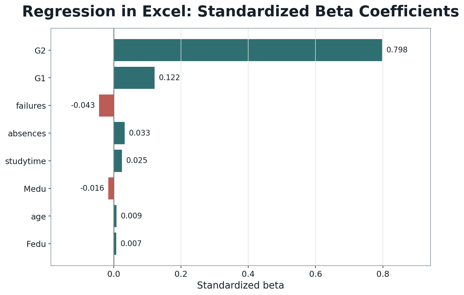
G2 dominates the fitted standardized comparison, while G1 is the only other coefficient with a visibly substantial positive bar.
G2 β = 0.797983, G1 β = 0.121852, failures β = −0.043219, absences β = 0.032697 and studytime β = 0.024811.
A one-standard-deviation difference in G2 is associated with the largest expected standardized G3 difference after adjustment for the remaining predictors.
Verify each bar with B × SD(X)/SD(Y), confirm the predictor range matches the coefficient label, and interpret standardized magnitude together with the confidence interval.
Regression in Excel Coefficient Interpretation
Regression in Excel coefficient interpretation must distinguish a conditional multiple-regression slope from a simple correlation.
An unstandardized coefficient is the expected G3 difference for a one-unit predictor contrast while the other listed predictors remain fixed. This conditional wording is essential for Regression in Excel because the simple and multiple coefficients answer different questions.
G2
The multiple-model G2 coefficient is 0.884807, with 95% CI [0.8173, 0.9523]. Holding G1, studytime, failures, absences, age, Medu and Fedu constant, a one-point G2 difference is associated with an expected 0.884807-point G3 difference. Its standardized beta of 0.797983 is the largest in the workbook.
G1
G1 has B = 0.143397 and 95% CI [0.0714, 0.2154]. Its coefficient is much smaller than the simple relationship expected from a prior grade because G1 overlaps strongly with G2. The multiple slope represents the increment associated with G1 among observations with the same G2 and other predictor values.
Failures
Failures has B = −0.235361 and 95% CI [−0.4224, −0.0484]. At matched values of the other predictors, one additional previous failure is associated with a lower expected G3. The standardized coefficient is modest, β = −0.043219.
Absences
Absences has B = 0.022762 and 95% CI [0.0013, 0.0442]. The coefficient is small and positive after adjustment, even though an unadjusted association may be negative. This suppression-style result reflects the fitted predictor set and must not be given a causal interpretation.
Uncertain coefficients
The saved 95% intervals for studytime, age, Medu and Fedu include zero. This does not prove that their population effects are exactly zero. It means that the fitted data and standard-error calculation do not isolate a sufficiently precise conditional association at the chosen confidence level.
Intercept
The intercept is −0.501155 with 95% CI [−2.0209, 1.0186]. It evaluates the equation when every predictor equals zero. Because that combination may not represent a realistic student profile, the intercept is necessary for prediction but may have limited substantive meaning.
Predictions, Contributions and Model Meaning
Regression in Excel prediction cells should expose each variable contribution before displaying the final fitted value.
The Prediction Calculator should place user inputs in the same order as the labeled coefficient vector. A safe design displays the input, coefficient and multiplication contribution on one row for each predictor, followed by the intercept and final SUMPRODUCT result.
Illustrative Excel Prediction
For an illustrative profile with G1 = 12, G2 = 11, studytime = 2, failures = 0, absences = 4, age = 18, Medu = 4 and Fedu = 4, the multiple equation gives:
| Term | Input | Coefficient | Contribution |
|---|---|---|---|
| Intercept | 1 | −0.501155 | −0.501155 |
| G1 | 12 | 0.143397 | 1.720764 |
| G2 | 11 | 0.884807 | 9.732877 |
| studytime | 2 | 0.096632 | 0.193264 |
| failures | 0 | −0.235361 | 0 |
| absences | 4 | 0.022762 | 0.091048 |
| age | 18 | 0.022685 | 0.408330 |
| Medu | 4 | −0.044951 | −0.179804 |
| Fedu | 4 | 0.022025 | 0.088100 |
| Predicted G3 | 11.553424 | ||
This profile is an illustration of the verified equation, not a new empirical result. Keep the full unrounded prediction for residuals and error metrics. A separately displayed rounded grade can be provided for convenience without replacing the analytical value.
Contribution Audit
A contribution table makes wrong references easier to detect. If the G2 input is multiplied by the G1 coefficient, the final prediction may still look plausible. Displaying each multiplication beside the variable label reveals the error immediately.
Prediction Versus Explanation
The workbook equation can support fitted prediction and conditional association. It does not establish an intervention effect. G2 may predict G3 strongly because it is a recent measurement of the same broader academic process, not because increasing a recorded G2 value mechanically causes a future increase of exactly 0.884807.
Regression in Excel Assumptions and Diagnostics
Regression in Excel diagnostics examine both statistical model weaknesses and spreadsheet implementation failures.
Workbook checks
- All model ranges contain the same 649 rows.
- Regression SS + residual SS = total SS.
- F = regression MS / residual MS.
- Predicted values match hand calculations.
- Residual = observed − predicted on every audited row.
- Charts point to complete live ranges.
Statistical checks
- Observed-versus-predicted alignment.
- Residual centering and curvature.
- Residual spread across fitted values.
- Unusual residuals and influential cases.
- G1 and G2 collinearity through VIF and tolerance.
- Performance on observations not used for fitting.
Linearity
The residual-versus-fitted chart should not show a systematic curve. If curvature is present, consider transformations, polynomial terms or a substantively justified alternative equation. Adding terms only because they improve fitted R² encourages overfitting.
Homoscedasticity
Residual spread should be reasonably stable across fitted values. A funnel pattern means conventional standard errors may be misleading. Excel can display the pattern, but the researcher must decide whether a variance adjustment or different model is needed.
Residual Normality
Normality is mainly relevant to classical confidence intervals and p values, especially in smaller samples. With 649 observations, mild departures may matter less for slope estimation than severe tails, influential cases or misspecification. Inspect the residual distribution rather than treating one test as the complete decision.
Independence
Independence comes from design and observation order. A row of formulas cannot detect every classroom, family, repeated-measurement or time dependence structure. When observations are clustered, an ordinary worksheet regression may understate uncertainty.
Multicollinearity
G1 and G2 measure related academic history, so their coefficients are conditional and may be sensitive to model composition. Review the Variance Inflation Factor guide and report VIF with tolerance. Do not remove a predictor automatically from one threshold without considering the research question.
Influence and Unusual Cases
Large residuals and unusual predictor profiles should be tied to case identifiers. Verify the source row before changing the model. Deletion is justified by a documented data error or a prespecified population rule, not because one case weakens R² or changes a p value.
Regression in Excel Procedures and Reproducibility
Regression in Excel reproducibility depends on documented ranges, settings, labels, protection and recalculation procedures.
Native worksheet functions
Best for a visible simple model and targeted audit formulas.
- SLOPE and INTERCEPT
- RSQ and CORREL
- STEYX and DEVSQ
- SUMPRODUCT predictions
- Observed-minus-predicted residuals
Analysis ToolPak
Best for a standard regression output block with ANOVA, coefficients and residual output.
- Record exact Y and X ranges.
- Document labels and confidence level.
- Keep the intercept unless intentionally constrained.
- Reconcile every slope with the workbook labels.
LINEST
Best for a formula-driven multiple-regression array.
- Known y must contain only eligible G3 rows.
- Known x must contain the eight aligned predictor columns.
- Coefficient order is reversed relative to x columns.
- Use the statistics argument to return fit evidence.
Protected worked workbook
Best for distribution to learners or clients.
- Mark editable cells clearly.
- Protect coefficients and formulas.
- Use automatic calculation.
- Retain a verified clean copy.
- Add visible row-count checks.
Recalculation Audit
- Open the workbook and confirm automatic calculation is active.
- Confirm 649 eligible rows on Data and each model sheet.
- Check the G3 outcome and eight predictor labels.
- Recalculate the workbook fully.
- Hand-check predictions for early, middle and late rows.
- Confirm residuals equal observed minus fitted.
- Reconcile ANOVA sums of squares and degrees of freedom.
- Verify standardized beta references the matching SD cells.
- Inspect chart series ranges.
- Save, reopen and compare headline cells with the verified report.
Excel Formulas and LINEST
Regression in Excel formulas below are representative audit formulas taken from the logic of the verified workbook.
Core simple-regression formulas
=COUNT(Data!$B$4:$B$652)
=SLOPE(Data!$B$4:$B$652,Data!$D$4:$D$652)
=INTERCEPT(Data!$B$4:$B$652,Data!$D$4:$D$652)
=CORREL(Data!$B$4:$B$652,Data!$D$4:$D$652)
=RSQ(Data!$B$4:$B$652,Data!$D$4:$D$652)
=STEYX(Data!$B$4:$B$652,Data!$D$4:$D$652)
These formulas use G3 as the y range and G2 as the x range. The range endpoints must remain identical.
Multiple-regression LINEST formula
=LINEST(Data!$B$4:$B$652,Data!$C$4:$J$652,TRUE,TRUE)In current Excel versions this can spill into an array. LINEST returns the slope coefficients in reverse order relative to the known x columns, followed by the intercept. Label the returned values explicitly before using them in a prediction equation.
Prediction and residual formulas
='Multiple Regression'!$E$4
 +'Multiple Regression'!$E$5*C4
 +'Multiple Regression'!$E$6*D4
 +'Multiple Regression'!$E$7*E4
 +'Multiple Regression'!$E$8*F4
 +'Multiple Regression'!$E$9*G4
 +'Multiple Regression'!$E$10*H4
 +'Multiple Regression'!$E$11*I4
 +'Multiple Regression'!$E$12*J4

=ObservedG3Cell-PredictedG3Cell
=ResidualCell^2
=ABS(ResidualCell)
Keep coefficient labels, input columns and row references synchronized. Do not round the fitted value before calculating the residual.
Model-fit formulas
=1-(1-RSquaredCell)*(NCell-1)/(NCell-KCell-1)
=RegressionSSCell+ResidualSSCell
=RegressionSSCell/RegressionDFCell
=ResidualSSCell/ResidualDFCell
=RegressionMSCell/ResidualMSCell
=SQRT(AVERAGE(SquaredResidualRange))
The RMSE formula above uses the mean of case-level squared residuals. Residual standard error uses a degrees-of-freedom denominator, so the two quantities should not be treated as interchangeable.
Standardized beta and confidence interval formulas
=CoefficientCell*STDEV.S(PredictorRange)/STDEV.S(OutcomeRange)
=CoefficientCell-TCriticalCell*StandardErrorCell
=CoefficientCell+TCriticalCell*StandardErrorCell
=CoefficientCell/StandardErrorCell
Use the t distribution and residual degrees of freedom for classical coefficient inference. A normal approximation may differ slightly, particularly when the sample is smaller.
Representative workbook audit formulas
Descriptive Statistics!B4
=COUNT(Data!$B$4:$B$652)

Descriptive Statistics!C4
=AVERAGE(Data!$B$4:$B$652)

Descriptive Statistics!D4
=STDEV.S(Data!$B$4:$B$652)

Correlation Matrix!C4
=CORREL(Data!$B$4:$B$652,Data!$C$4:$C$652)

Diagnostics!K4
='Multiple Regression'!$E$4
 +'Multiple Regression'!$E$5*C4
 +'Multiple Regression'!$E$6*D4
 +'Multiple Regression'!$E$7*E4
 +'Multiple Regression'!$E$8*F4
 +'Multiple Regression'!$E$9*G4
 +'Multiple Regression'!$E$10*H4
 +'Multiple Regression'!$E$11*I4
 +'Multiple Regression'!$E$12*J4

Diagnostics!L4
=B4-K4
The complete workbook contains the filled-row pattern. The important audit question is whether each formula continues consistently through row 652 without a broken or shifted reference.
Advanced Regression in Excel Topics
Regression in Excel requires additional care when LINEST arrays, changing ranges, collinearity and future prediction claims are involved.
ToolPak Versus LINEST
The Analysis ToolPak produces a familiar output block, while LINEST creates a formula-based result that can update with the source ranges. ToolPak is easier to read initially; LINEST is easier to embed in a controlled workbook. Both should produce the same coefficients when they use the same rows, intercept rule and predictor order.
LINEST Coefficient Order
LINEST returns slopes in reverse order. For known x columns C:J, the first returned slope corresponds to column J, not column C. A workbook can therefore contain numerically correct LINEST output but a mislabeled equation. Always build a label row from the known x order and verify one prediction manually.
Simple Versus Multiple Fit
The simple model has R² = 0.843730 and the multiple model has R² = 0.850777. The modest gain demonstrates that more predictors do not automatically create a substantially better model. The additional variables are most useful when conditional interpretation is substantively required.
R², Adjusted R² and RMSE
R² measures fitted proportional variation, adjusted R² penalizes predictor count, and RMSE expresses error in G3 units. These measures answer different questions. A model can have high R² and still make important errors for boundary outcomes or particular subgroups.
Suppression and Sign Changes
The positive absences coefficient is a warning against reading a multiple slope as a raw association. When predictors share information, adjustment can reduce, enlarge or reverse a coefficient. Inspect the correlation matrix and compare simple and multiple slopes before writing a substantive explanation.
Confidence Intervals Over Display Stars
Confidence intervals communicate direction and uncertainty more clearly than significance symbols alone. Report B, SE or interval, units and conditioning variables. The overall F test concerns the complete predictor block; it does not imply that every separate slope excludes zero.
Structured Tables and Dynamic Ranges
Fixed ranges make the verified workbook reproducible, but a structured Excel table is safer when new rows will be added. All formulas, charts and validation checks must then use the same table columns and a documented complete-case method.
Spreadsheet Governance
Protect formula cells, use data validation where possible, avoid merged cells inside calculation tables, maintain a visible change log and retain an untouched benchmark copy. A workbook without governance can change silently while continuing to display plausible statistics.
In-Sample Fit Versus Future Accuracy
The saved RMSE is calculated from the same 649 observations used to estimate the slopes. Honest predictive evaluation requires unseen observations or repeated resampling. Do not rename fitted RMSE as test RMSE or expected future error.
Common Regression in Excel Mistakes
Formula and range mistakes
- Using different start or end rows across variables.
- Sorting one column without the complete table.
- Overwriting a formula with a pasted constant.
- Reversing LINEST coefficient labels.
- Rounding predictions before residual calculation.
- Extending data without extending charts or formulas.
Interpretation mistakes
- Calling a conditional coefficient causal.
- Calling fitted RMSE future accuracy.
- Assuming high R² proves the workbook is correct.
- Deleting every predictor with p > .05 automatically.
- Treating standardized beta as universal importance.
- Ignoring residual and collinearity evidence.
Decision Rules for Spreadsheet Users
- Use one controlled analysis frame and display the complete-case count.
- Verify at least three predictions by hand.
- Reconcile sums of squares, degrees of freedom and F.
- Interpret confidence intervals before simplifying the model.
- Investigate unusual rows before deletion.
- Separate fitted description from validation claims.
- Protect calculation cells before sharing the workbook.
- Regression in Excel should display the complete-case count beside every model summary.
- Regression in Excel should preserve one predictor order from estimation through prediction.
- Regression in Excel should use unrounded fitted values for residuals and RMSE.
- Regression in Excel should reconcile regression, residual and total sums of squares.
- Regression in Excel should protect coefficient and diagnostic formulas before distribution.
- Regression in Excel should document whether results came from LINEST, ToolPak or verified cells.
- Regression in Excel should treat fitted RMSE as in-sample evidence until validation is performed.
- Regression in Excel should retain case identifiers when residuals are sorted or filtered.
- Regression in Excel should report confidence intervals rather than significance labels alone.
- Regression in Excel should keep causal language within the limits of the study design.
APA-Style Reporting
Regression in Excel reporting should identify the exact equation, complete-case count, fit statistics and evidence limitations.
State that the reported error is fitted-sample error unless a separate validation analysis exists. Also state whether coefficients came from the ToolPak, LINEST or stored verified workbook cells.
Publication Checklist
Regression in Excel publication checks should be completed before the workbook or article is released.
- Use the exact focus phrase Regression in Excel naturally in the title, introduction and major explanations.
- State G3 as the outcome and list all eight multiple predictors.
- Report the 649-row complete-case count.
- Include the simple and multiple equations.
- Distinguish R², adjusted R², residual standard error and fitted RMSE.
- Report ANOVA degrees of freedom and the overall F test.
- Report B, confidence intervals and standardized beta with correct labels.
- Explain the conditional absences coefficient cautiously.
- Verify that chart series use live Excel ranges.
- Check workbook formulas for broken references and inconsistent endpoints.
- Protect calculation cells and preserve a verified copy.
- Limit causal and future-prediction claims to the available evidence.
- Verify workbook and report download links.
- Retain all advertisement placements and the back-to-top control.
Downloads and Excel Chart Resources
Regression in Excel downloads are limited here to the verified workbook, report and workbook-based visual assets.
The downloadable evidence is limited to the verified Excel workbook, the Excel reading report and the three workbook-based chart assets. No unrelated software output is presented.
regression_in_excel_verified_report.pdfVerified four-page Excel regression report
Observed versus predicted chartExcel model agreement visual
Residuals versus fitted chartExcel residual-pattern visual
Standardized beta chartExcel coefficient-scale comparison
Frequently Asked Questions
Regression in Excel questions below focus on the workbook decisions most likely to change the reported result.
Can Excel perform multiple regression without the Analysis ToolPak?
Yes. LINEST can estimate the coefficient array, and a controlled workbook can use stored coefficients with formulas for predictions, residuals, fit summaries, standardized betas and charts. The predictor order must be documented carefully.
Why are the simple-sheet p values described cautiously?
The displayed simple-sheet probability calculation can use a normal approximation while confidence limits use a stored t critical value. For formal reporting, use the residual degrees of freedom and the t distribution consistently.
What is the difference between STEYX and RMSE?
STEYX is the residual standard error for a simple regression using its degrees-of-freedom convention. The workbook’s case-level RMSE is the square root of the average squared residual. Their denominators differ, so their values are not interchangeable.
Why is G2 the strongest predictor?
Its standardized beta is 0.797983, much larger in absolute value than the other saved betas, and its 95% confidence interval excludes zero. This conclusion applies to the fitted predictor set and sample.
Why is the absences coefficient positive?
It is a conditional coefficient after adjustment for G1, G2, failures and the remaining predictors. Shared predictor information can reverse a zero-order association. The coefficient is not evidence that absence improves grades.
May I round the predicted grade?
A rounded value can be displayed for convenience, but residuals, RMSE, sums of squares and diagnostic charts must use the unrounded prediction.
How should new rows be added?
Extend the outcome and all predictor ranges together, recalculate every sheet, inspect chart sources and repeat the benchmark checks. Converting the source range to a structured Excel table reduces endpoint errors.
Does a high R² prove the workbook is correct?
No. High R² describes fitted association. Wrong ranges, reversed coefficient labels, outcome leakage, dependence, overwritten formulas or an inappropriate model can remain.
Which cells should users edit?
Only clearly marked source-data and prediction-input cells should be editable. Coefficient, ANOVA, diagnostic, formula and dashboard cells should be protected in the distributed copy.
Can fitted RMSE be reported as future prediction error?
No. Fitted RMSE uses the same observations that estimated the equation. Future accuracy requires a separate test set or a resampling design.
Regression in Excel remains the focus throughout this guide because Regression in Excel includes more than pressing the Regression button. A defensible Regression in Excel workbook connects data ranges, coefficients, predictions, residuals, ANOVA, confidence intervals, standardized effects and protected formulas. Used carefully, Regression in Excel makes the complete calculation trail visible.
Regression in Excel Conclusion
Regression in Excel is defensible when its numerical accuracy and its spreadsheet architecture are verified together.
Regression in Excel provides a strong and auditable fitted model when every range, formula, label and diagnostic cell is controlled. In the worked file, G2 alone explains most fitted G3 variation. The eight-predictor equation raises R² from 0.843730 to 0.850777 and reduces fitted error, while preserving G2 as the dominant standardized predictor.
The most defensible interpretation combines the fit statistics with coefficient uncertainty and workbook limitations. G1 and G2 have positive conditional coefficients, failures has a negative coefficient, and absences has a small positive adjusted coefficient that should not be interpreted causally. The spreadsheet is valuable because predictions, residuals and ANOVA can be traced, but that traceability does not replace study design or external validation.

