
Random Effects Regression: Formula, ICC, Interpretation, Python, R, SPSS and Excel
Random Effects Regression models repeated or grouped observations by combining population-average fixed effects with cluster-specific random variation. This verified example reshapes G1, G2 and G3 for 649 students into 1,947 grade-period records and explains the random student intercept, fixed effects, variance components, intraclass correlation, likelihood comparison, predictions and diagnostics across Python, R, SPSS and Excel.
Random Effects Regression Model Overview
Random Effects Regression is a mixed-model method for outcomes measured repeatedly or observed inside meaningful clusters. It combines a population-average fixed equation with random cluster deviations, allowing records from the same student, school, clinic, firm or household to remain statistically related rather than being treated as independent rows.
The worked outcome is grade_score. The original G1, G2 and G3 columns are stacked into long format, producing 1,947 grade-period records from 649 students. Each student contributes three observations. The fixed part includes grade period, studytime, failures, absences, age, Medu, school, sex and address. A student-specific random intercept shifts all three fitted grades for that student upward or downward.
The research question is: how do grade period and student characteristics relate to repeated grade scores after accounting for persistent between-student differences? The fixed coefficients answer average conditional questions. The random-intercept variance measures remaining heterogeneity among students, while residual variance measures remaining within-student and occasion-specific variation.
When Random Effects Regression Is Appropriate
Use Random Effects Regression when several observations belong to the same unit, a cluster-specific deviation is scientifically meaningful, and the analyst wants both average fixed effects and a probabilistic description of cluster heterogeneity. The method is part of the broader Mixed Effects Regression family and is often presented through the level-1 and level-2 notation of a Hierarchical Linear Model.
Do not apply the model automatically merely because a grouping variable exists. The response distribution must suit a Gaussian mixed model, enough clusters must be available, the random structure must reflect the design, and the assumption that random effects are independent of the included predictors must be defensible. When that independence assumption is implausible and the target is strictly within-cluster change, Fixed Effects Regression may answer a more appropriate question.
Random-Intercept Formula
Index i identifies the grade occasion and j identifies the student. The fixed term x′β describes the average adjusted mean. The shared random intercept u0j induces covariance among G1, G2 and G3 from the same student.
The ICC indicates that two conditionally comparable grade records from the same student have an estimated correlation of about 0.815 under this random-intercept covariance structure. The Intraclass Correlation Coefficient is a variance partition, not a mixed-model R squared and not the percentage of grade variation explained by the fixed predictors.
Assumptions
Students are independent clusters, while repeated grade records may be dependent within students.
Grade-period indicators and numeric predictors adequately describe the conditional mean.
A shared student intercept is sufficient; the current model does not contain random slopes.
Additional assumptions concern approximately Gaussian conditional residuals and random intercepts, stable variance components, correctly specified reference groups and independence between the random intercept and included predictors. Diagnostics must examine both observation-level residuals and student-level empirical random effects.
Advantages and Limitations
The advantages are proper handling of repeated observations, partial pooling of student effects, separation of between-student and within-student variation, and explicit distinction between population-level and known-student predictions. Limitations include dependence on the random-effects distribution, possible bias when cluster effects correlate with predictors, optimistic in-sample conditional prediction, and the inability of a random intercept alone to represent different student-specific rates of change.
The full model improves the null random-intercept model by likelihood-ratio χ²(10) = 299.8452, p = 1.6763 × 10−58. Student variance is 5.235425 and residual variance is 1.187727. These results establish that clustering is central to the worked analysis, while the fixed-effect table identifies the average adjusted associations.
Quick Answer
The verified Random Effects Regression model contains 649 student clusters and 1,947 repeated grade records. The random student intercept captures substantial persistent heterogeneity, and the fixed-effect block improves the null mixed model decisively.
Why the grouped model is necessary
- Every student contributes G1, G2 and G3.
- Student variance is 4.407936 times residual variance.
- Pooled Ordinary Least Squares Regression treats the 1,947 rows as independent.
- The random intercept preserves within-student covariance and supplies partial pooling.
What the fitted model reports
- G2 is 0.1710 points above G1 after adjustment.
- G3 is 0.5069 points above G1 after adjustment.
- Each failure is associated with 1.5189 fewer grade points.
- studytime is associated with 0.4603 higher grade points per coded level.
Table of Contents
- Quick Answer
- Why This Analysis Needs Random Effects Regression
- How Random Effects Regression Works
- Variables and Coding
- Verified Results
- Python Chart Stories
- R Chart Pairs
- Coefficient and Variance Interpretation
- Predictions and Model Meaning
- Assumptions and Diagnostics
- Python, R, SPSS and Excel
- Code
- Advanced Topics
- APA-Style Reporting
- Publication Checklist
- Downloads
- Related Guides
- Frequently Asked Questions
- Conclusion
Why This Analysis Needs Random Effects Regression
G1, G2 and G3 are repeated measurements of the same grade construct. Reshaping the wide table creates student_id, grade_period and grade_score. The grade-period record is the level-1 observation, while the student is the level-2 cluster.
A pooled linear regression estimates one fixed equation but assumes that residuals from different rows are independent. With ICC 0.815087, that simplification is not a minor technical issue. Repeated observations from one student share a large common component, so pooled standard errors, prediction interpretation and effective information can be misleading.
Random Effects Regression introduces a partially pooled student intercept. A positive empirical intercept raises all three fitted grades for that student; a negative value lowers them. The estimate is shrunk toward zero according to the amount of information and the estimated variance components. It is not a raw student mean, a causal ability score or a permanent ranking.
The model also separates two prediction questions. A conditional fitted value for a known student uses the estimated student deviation. A population-level prediction for a new student uses the fixed equation and initially sets the unknown random effect to zero. This distinction is central to fair evaluation and is explained further in the Mixed Effects Regression guide.
How Random Effects Regression Works
Long-Format Equation
G1 is the reference period. The G2 and G3 indicators therefore estimate adjusted departures from G1. Vector z contains studytime, failures, absences, age, Medu, school, sex and address. The random intercept is shared by all three rows belonging to student j.
Stack G1, G2 and G3, retain student_id and declare all reference groups.
Fit fixed coefficients, student variance and residual variance jointly.
Combine likelihood evidence, ICC, coefficients, residuals and cluster-level prediction.
Variance and Covariance
For two grade records from the same student, the covariance is σ²u because both contain the same random intercept. Their total conditional variance is σ²u + σ²e. The random-intercept model therefore implies one common within-student correlation, often called a compound-symmetry structure.
The fitted student variance of 5.235425 is much larger than residual variance 1.187727. That decomposition explains the high ICC and the large difference between conditional mixed-model error and pooled OLS error.
Maximum Likelihood and the Likelihood-Ratio Test
The null and full models contain the same student random intercept but different fixed-effect structures. Because fixed effects change, the reported likelihood-ratio comparison uses maximum likelihood rather than REML. The statistic is 2[−3791.6762 − (−3941.5988)] = 299.8452 on 10 degrees of freedom.
REML is often preferred for estimating variance components after the fixed specification has been chosen, but REML likelihoods from models with different fixed terms are not directly comparable. The article keeps model selection and final estimation conventions explicit rather than mixing them.
Partial Pooling
Student random-intercept predictions combine the student’s observed grade information with the population distribution. Students with little reliable information are pulled more strongly toward zero. Partial pooling reduces the instability of 649 separate unpooled intercept estimates while preserving meaningful cluster heterogeneity.
Core Assumptions
Different students are independent under the sampling design.
After fixed and random terms, occasion-level errors have an adequate mean and variance structure.
Student intercepts are approximately Gaussian and independent of the included predictors.
Linearity is required for numeric terms on the conditional mean scale. The model also assumes that one random intercept adequately represents within-student dependence. Use Regression Diagnostics together with cluster-level checks rather than relying only on convergence.
Variables Used, Coding and Standardization
The long-format coding corresponds to a two-level Hierarchical Linear Model: occasions are nested within students. G1, GP school, female sex and rural address are the reference categories.
| Role | Variable | Coding used | Coefficient interpretation |
|---|---|---|---|
| Outcome | grade_score | Values reshaped from G1, G2 and G3 | Continuous repeated grade |
| Occasion | grade_period | G1 reference; G2 and G3 indicators | Adjusted period difference from G1 |
| Numeric predictor | studytime | Original study-time code | Expected grade change for one category |
| Numeric predictor | failures | Previous failure count/code | Expected grade change per failure unit |
| Numeric predictor | absences | Absence count | Expected grade change per absence |
| Numeric predictor | age | Age in years | Expected grade change per year |
| Numeric predictor | Medu | Mother’s education code | Expected grade change per education level |
| Categorical predictor | school | GP reference; MS indicator | MS minus GP adjusted mean |
| Categorical predictor | sex | Female reference; male indicator | Male minus female adjusted mean |
| Categorical predictor | address | Rural reference; urban indicator | Urban minus rural adjusted mean |
| Cluster | student_id | 649 unique students | Defines the shared random intercept |
The fixed intercept of 9.9855 refers to G1, GP school, female and rural when all numeric predictors equal zero. Because age zero is impossible and other zero values may be uncommon, centering numeric variables would provide a more meaningful intercept without changing fitted values.
Grade period is categorical. G2 and G3 therefore estimate separate departures from G1 and do not impose equal linear change across periods.
Verified Random Effects Regression Results
Model Fit and Likelihood Comparison
The full and null mixed models use the same 1,947 records and 649 student clusters. The full model log likelihood is −3791.6762 compared with −3941.5988 for the null random-intercept model. The likelihood-ratio statistic is 299.8452 on 10 degrees of freedom, p = 1.6763 × 10−58. Lower AIC and BIC also favor the prespecified fixed-effect block.
The pooled Ordinary Least Squares Regression comparison has much larger error because it omits the student-specific intercept. Its R squared of 0.2744 belongs to the pooled comparison and must not be presented as marginal or conditional mixed-model R squared.
| Model | Log likelihood | AIC | BIC | RMSE | MAE | Specification |
|---|---|---|---|---|---|---|
| Null random-intercept model | −3941.5988 | 7889.1976 | 7905.9198 | 0.9263 | 0.6350 | Intercept plus student random intercept |
| Full Random Effects Regression | −3791.6762 | 7609.3524 | 7681.8150 | 0.9053 | 0.6056 | Ten fixed-effect degrees of freedom plus student random intercept |
| Pooled OLS comparison | −4573.2949 | 9168.5898 | 9229.9043 | 2.5344 | 1.9029 | Treats all 1,947 rows as independent |
Variance Components and ICC
Student random-intercept variance is 5.235425, residual variance is 1.187727 and total conditional variance is 6.423152. The resulting ICC is 0.815087. The random-intercept standard deviation of 2.288106 is more than twice the residual standard deviation of 1.089829.
This variance evidence supports a grouped model, but it does not determine whether a random slope is required. That decision needs trajectory patterns, estimability, model comparison and validation.
| Component | Estimate | Share or ratio | Interpretation |
|---|---|---|---|
| Student random-intercept variance | 5.235425 | 81.5087% | Persistent adjusted differences among student baselines |
| Residual variance | 1.187727 | 18.4913% | Remaining within-student and occasion-specific variation |
| Total conditional variance | 6.423152 | 100.0000% | Denominator used in the ICC |
| Random-intercept SD | 2.288106 | — | Typical scale of persistent student deviation |
| Residual SD | 1.089829 | — | Typical conditional occasion-level deviation |
| Variance ratio | 4.407936 | — | Between-student variance divided by residual variance |
Fixed-Effect Coefficients
Using G1 as the grade-period reference, adjusted G2 is 0.1710 points higher and adjusted G3 is 0.5069 points higher. Failures has the largest absolute numeric slope at −1.5189. studytime and Medu are positive, while absences, MS school and male sex are negative. The age and urban-address intervals include zero.
Every coefficient is conditional on the student random intercept and the remaining fixed terms. These observational associations should not be converted into causal intervention effects.
| Term | Coefficient | SE | 95% CI | p-value | Interpretation |
|---|---|---|---|---|---|
| Intercept | 9.9855 | 1.4049 | [7.2320, 12.7389] | 1.18 × 10⁻¹² | Reference-profile anchor |
| G2 versus G1 | 0.1710 | 0.0605 | [0.0525, 0.2896] | 0.0047 | Small positive adjusted period difference |
| G3 versus G1 | 0.5069 | 0.0605 | [0.3884, 0.6255] | <.0001 | Positive adjusted period difference |
| MS versus GP school | −1.2709 | 0.2202 | [−1.7024, −0.8393] | 7.82 × 10⁻⁹ | Lower adjusted grade for MS |
| Male versus female | −0.5788 | 0.1971 | [−0.9652, −0.1924] | 0.0033 | Lower adjusted grade for males |
| Urban versus rural | 0.2820 | 0.2181 | [−0.1456, 0.7095] | 0.1961 | Interval includes zero |
| studytime | 0.4603 | 0.1186 | [0.2278, 0.6929] | 0.0001 | Positive adjusted association |
| failures | −1.5189 | 0.1707 | [−1.8534, −1.1844] | <.0001 | Largest absolute numeric slope |
| absences | −0.0657 | 0.0210 | [−0.1068, −0.0246] | 0.0017 | Small negative effect per absence |
| age | 0.0393 | 0.0819 | [−0.1213, 0.1999] | 0.6316 | Interval includes zero |
| Medu | 0.3690 | 0.0873 | [0.1978, 0.5402] | 0.000024 | Positive adjusted association |
Open the Main Output Files
The same verified files appear again in Downloads.
Python Charts and Explanations
The six distinct Python assets are each used once and explained through the visible pattern, exact values, statistical meaning and next verification step.
Python Chart 1: Variance Components and Intraclass Correlation
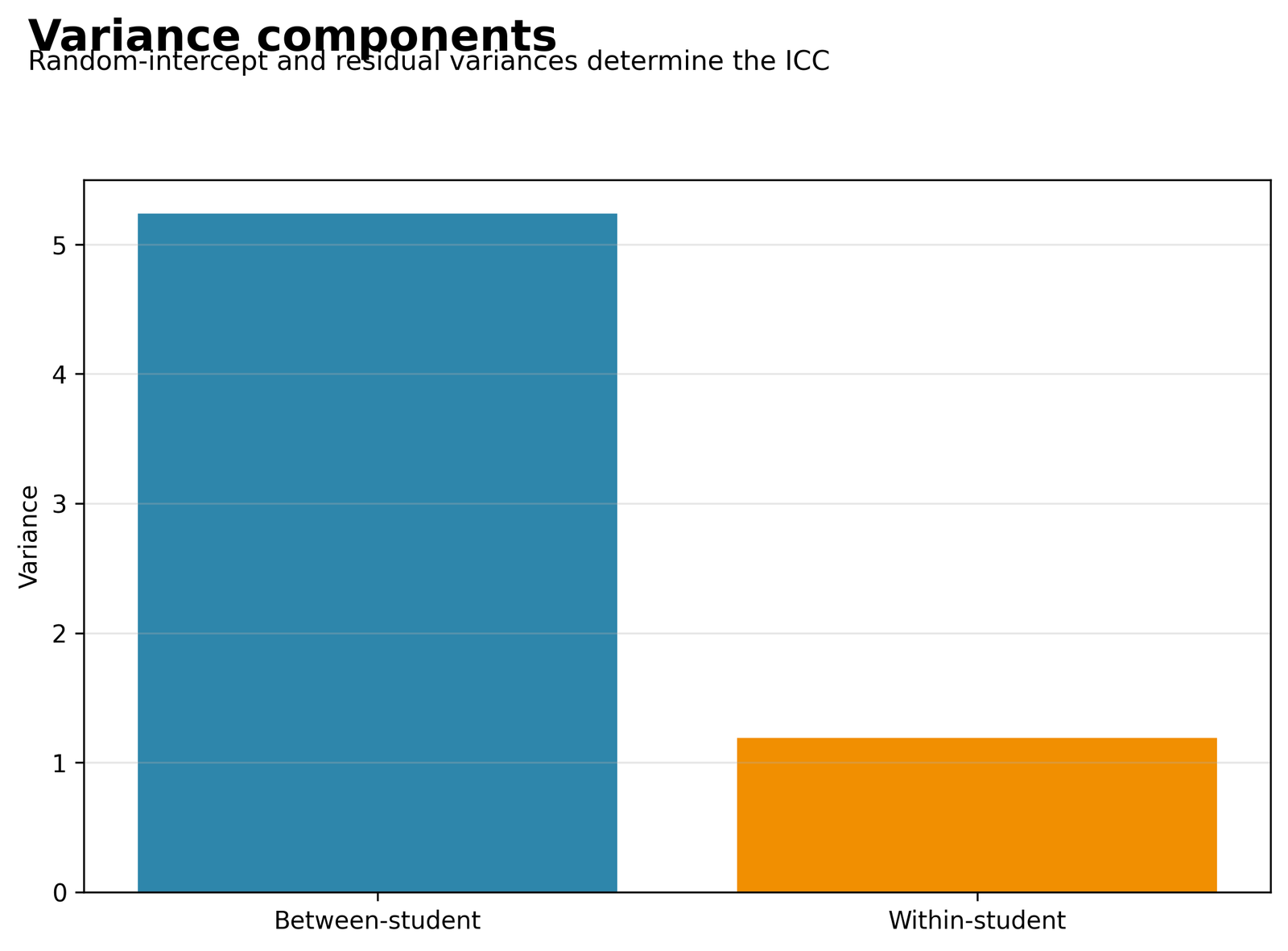
The chart compares persistent between-student variation with remaining within-student and occasion-level variation.
Random-intercept variance = 5.235425, residual variance = 1.187727, total variance = 6.423152 and ICC = 0.815087.
Two grade records from the same student have an estimated conditional correlation of about 0.815 under the random-intercept covariance structure.
Use the Intraclass Correlation Coefficient guide and verify that the ICC is reported as a variance partition rather than an R-squared.
Python Chart 2: Fixed-Effect Coefficients and Confidence Intervals
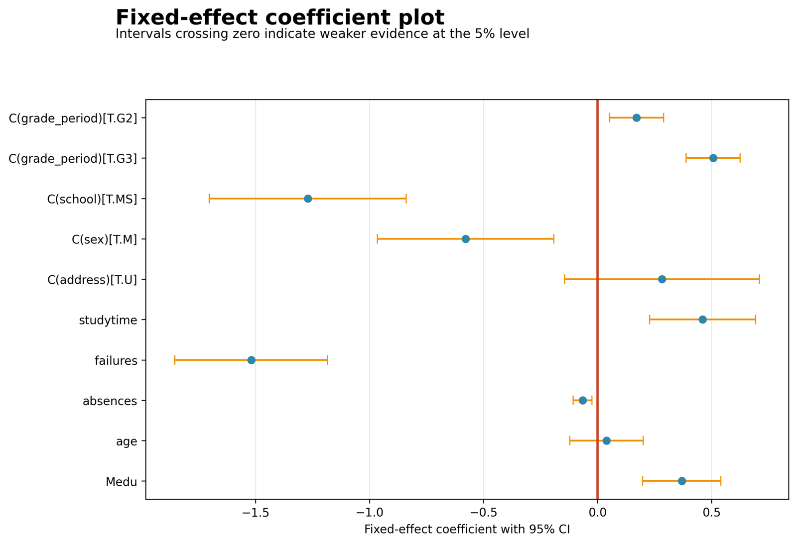
The chart places positive and negative fixed effects around the zero reference and displays their uncertainty.
failures = −1.5189, school_MS = −1.2709, G3 versus G1 = 0.5069, studytime = 0.4603 and Medu = 0.3690.
Failures has the largest absolute numeric slope. Urban address and age have intervals spanning zero, while the other displayed supported effects retain their stated coding.
Read every interval against zero and confirm the reference groups before describing effect direction or magnitude.
Python Chart 3: Distribution of Student Random Intercepts
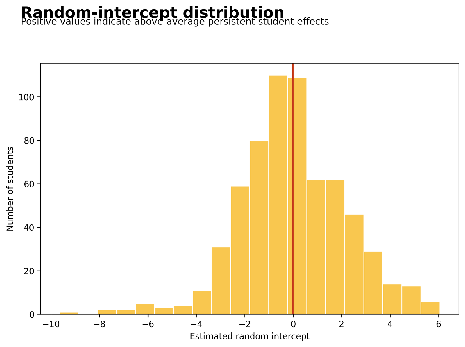
The distribution is centered near zero because random effects are modeled as deviations from the population intercept.
Random-intercept variance = 5.235425 and SD = 2.288106. Example estimates include student 1 = −5.5791, student 2 = −1.8466 and student 3 = 0.3301.
The estimates are partially pooled model-based deviations. They are not raw student means, causal ability scores or permanent rankings.
Inspect the caterpillar plot and remember that shrinkage depends on the fitted fixed effects, variance components and available repeated measurements.
Python Chart 4: Observed versus Conditional Fitted Grades
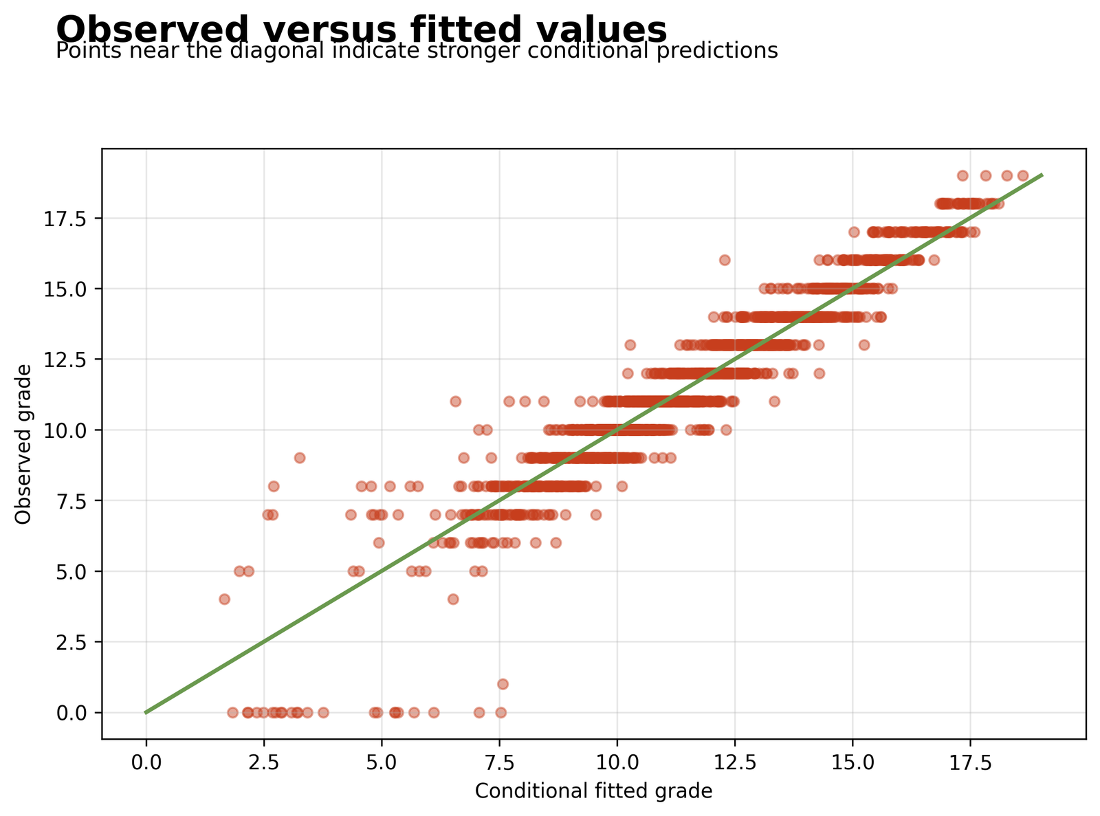
The graph compares actual grade_score with fitted values that use both the fixed equation and the estimated student deviation.
Full conditional RMSE = 0.9053 and MAE = 0.6056. Pooled OLS RMSE = 2.5344 and MAE = 1.9029.
The large improvement partly reflects access to each known student’s other grade information. It is not prospective accuracy for a completely new student.
Validate new-student performance by holding out entire student_id clusters and predicting without their unavailable random effects.
Python Chart 5: Conditional Residual Distribution
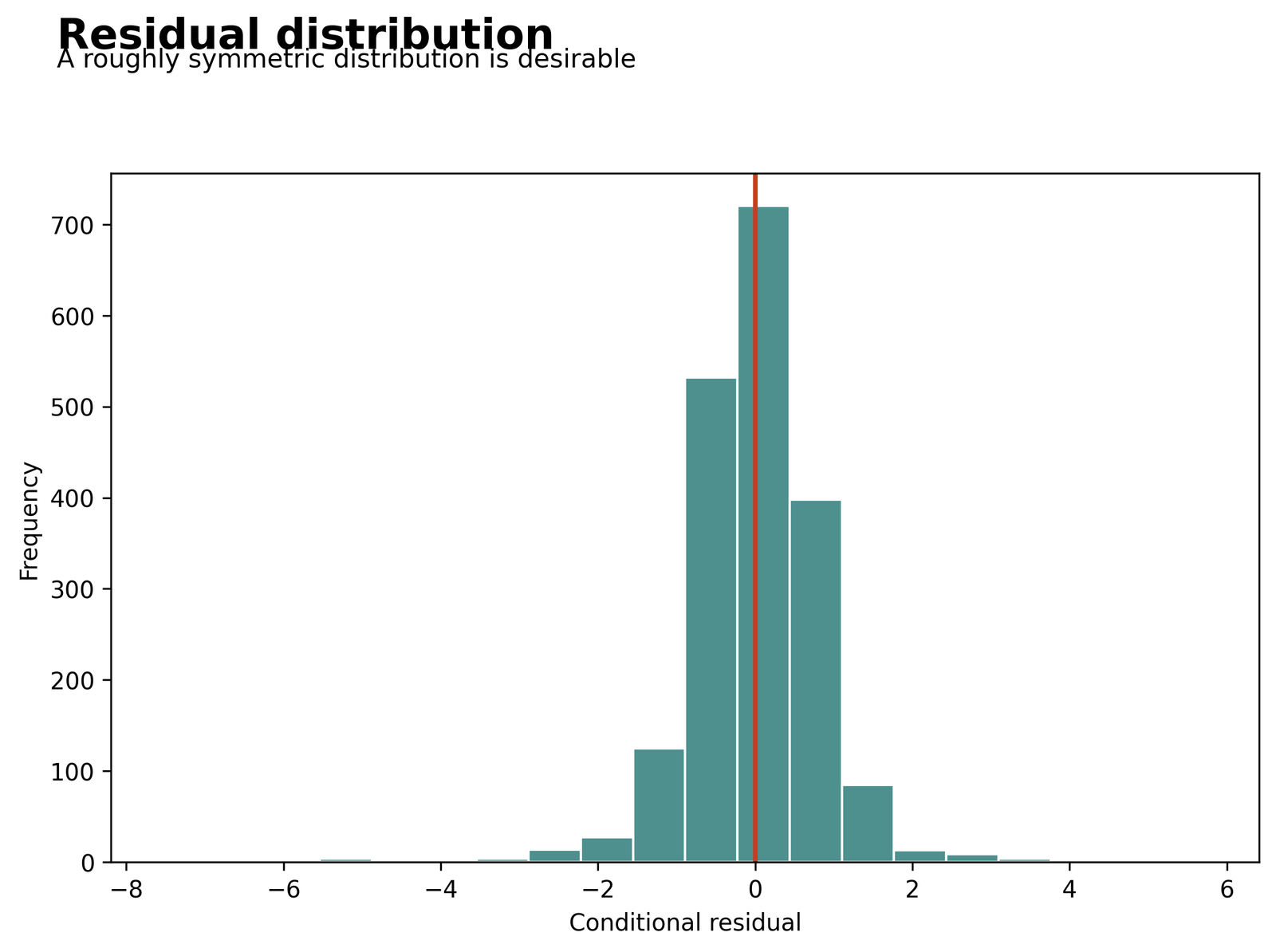
The chart checks centering, tail behavior and possible concentrations caused by bounded integer grade values.
Residual variance = 1.187727, residual SD = 1.089829, conditional RMSE = 0.9053 and MAE = 0.6056.
Raw grades do not need to be normal. The relevant distribution is the conditional residual after the student effect and fixed terms are included.
Compare the histogram with residual-versus-fitted and Q-Q evidence, and investigate valid zero-grade records rather than deleting them automatically.
Python Chart 6: Mean Grade by Period
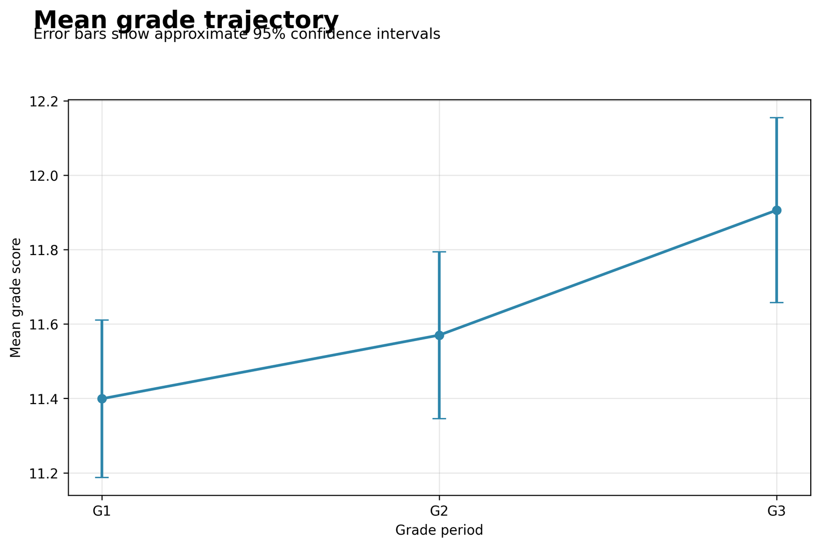
The chart displays the overall grade pattern across G1, G2 and G3 before or alongside covariate adjustment.
Using G1 as the reference, the adjusted G2 coefficient is 0.1710 with 95% CI [0.0525, 0.2896], and the adjusted G3 coefficient is 0.5069 with 95% CI [0.3884, 0.6255].
Marginal means and adjusted mixed-model coefficients answer related but different questions. The period coefficients control the listed covariates and student intercept.
Compare this structure with Repeated Measures ANOVA and avoid assuming equal change between consecutive periods.
R Charts and Explanations
The four unique R assets are organized into two paired rows. Each chart appears once and stacks directly above its matching explanation on mobile.
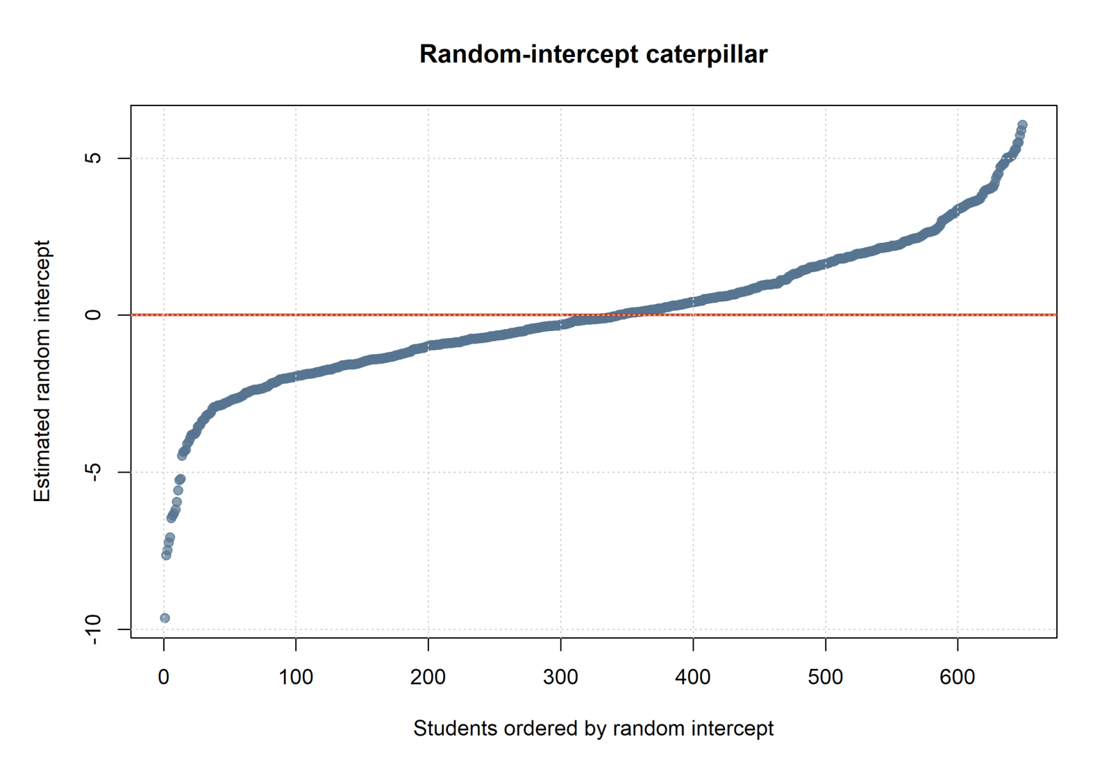
R Chart 1: Student Random-Intercept Caterpillar Plot
The sorted estimates show the spread of persistent adjusted student deviations. Extreme-looking values remain shrunken toward zero and have different estimation uncertainty.
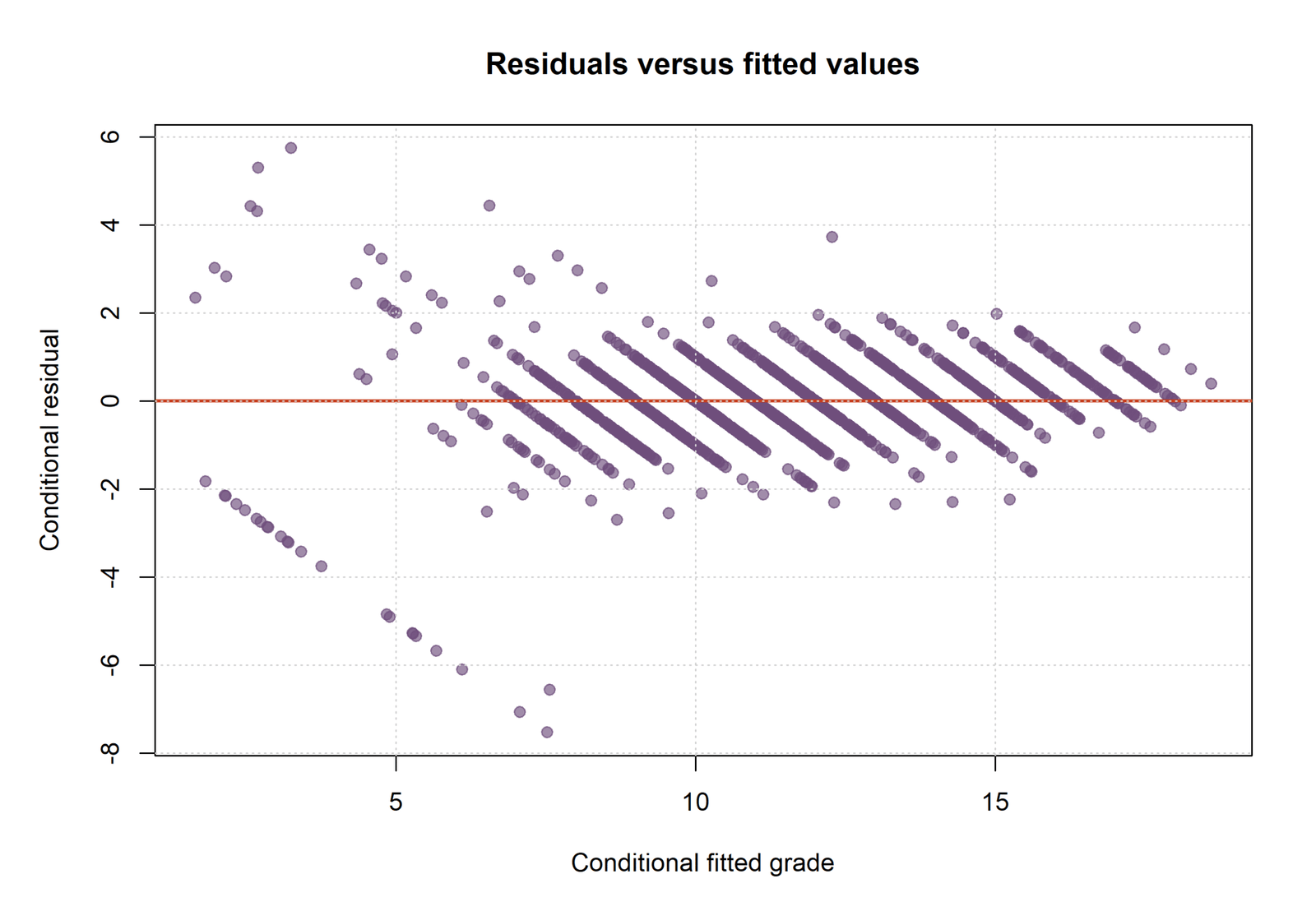
R Chart 2: Conditional Residuals versus Fitted
The plot checks whether the fixed mean equation and residual variance remain adequate after the student random intercept is included.
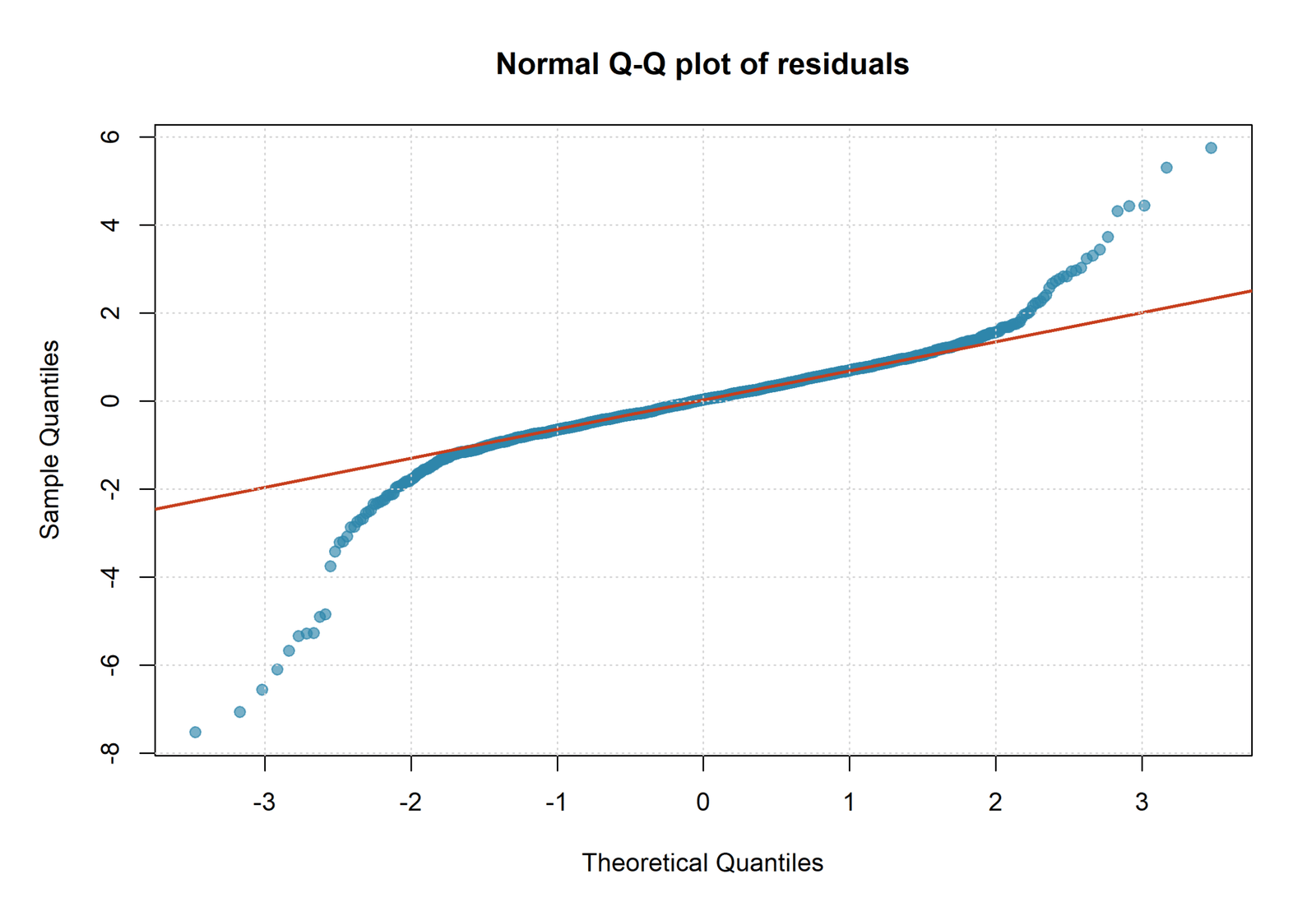
R Chart 3: Conditional Residual Q-Q Plot
Central alignment supports approximate normal behavior in the main body, while lower- or upper-tail departures identify grade records that need verification and sensitivity analysis.
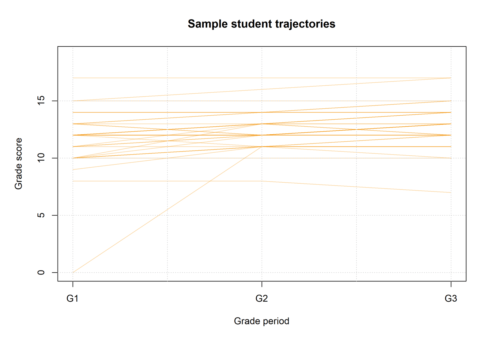
R Chart 4: Sample Student Trajectories
Individual profiles show why the three grade records from one student are dependent. A random intercept shifts the whole trajectory but does not allow student-specific slopes.
Random Effects Regression Coefficient and Variance Interpretation
Grade-Period Effects
Relative to G1, G2 is 0.1710 points higher, 95% CI [0.0525, 0.2896], and G3 is 0.5069 points higher, 95% CI [0.3884, 0.6255], after adjustment. The period effect is categorical; the model does not force equal change between G1, G2 and G3.
Student Characteristics
One additional failure unit is associated with 1.5189 fewer expected grade points, 95% CI [−1.8534, −1.1844]. studytime is associated with 0.4603 higher points per coded level, and Medu is associated with 0.3690 higher points per education-code step. Each absence is associated with 0.0657 lower points.
MS school is 1.2709 points below GP, and male is 0.5788 points below female after adjustment. The urban-versus-rural estimate is 0.2820 with an interval crossing zero. Age also has an interval crossing zero.
Variance Parameters
The random-intercept variance is 5.235425 and residual variance is 1.187727. Their standard deviations are 2.288106 and 1.089829. The resulting Intraclass Correlation Coefficient of 0.815087 describes conditional similarity among repeated grades from the same student.
Random Effects Regression coefficients and variance components answer different questions. Fixed coefficients describe average adjusted mean differences. Variance components describe remaining heterogeneity and dependence. Neither quantity should be substituted for the other.
Predictions, Effects and Model Meaning
Conditional Prediction
The empirical student deviation is estimated from that student’s observed grades. Conditional fitted values are useful for describing known students and checking the fitted model, but their in-sample accuracy partly reflects information borrowed from the same cluster.
Population-Level Prediction
A completely new student has no estimated random intercept. The initial prediction therefore uses the fixed equation and treats the expected random deviation as zero. Prediction uncertainty should include both residual variance and the distribution of possible student effects.
Why Row-Wise Splitting Leaks Information
A random row split can place G1 and G2 for one student in training while G3 for the same student appears in testing. The model then gains indirect information about the held-out record through the student intercept. New-student evaluation must split by student_id, not by grade-period row.
The Repeated Measures ANOVA guide provides a more restrictive repeated-mean comparison, while this model supports covariates, incomplete repeated records under likelihood assumptions and student-specific partial pooling.
Random Effects Regression Assumptions and Diagnostics
Inspect conditional residuals, fitted-value patterns, period-specific spread and unusual grade records.
Inspect empirical student effects, influential clusters and variance-component stability.
Evaluate whether a random intercept alone is adequate or whether slopes and covariance need expansion.
Conditional Residuals
Residuals should be centered around zero without strong curvature or a large change in spread. Because grades are bounded and integer-valued, visible bands can occur even when the mean structure is reasonable. The residual distribution and Q-Q plot should be interpreted together rather than requiring perfect normality.
Random-Effect Distribution
The histogram and caterpillar plot assess whether the Gaussian random-intercept approximation is plausible and whether a small number of students appear unusually influential. Empirical random effects are shrunken predictions with unequal uncertainty, not directly observed parameters.
Influence at Two Levels
An unusual grade occasion can affect one residual, while a consistently unusual student can affect fixed slopes and variance components. Leave-one-student-out refits are more appropriate than deleting isolated rows without considering the cluster.
Functional Form and Variance
studytime, failures, absences, age and Medu are entered linearly. Residual curvature can indicate omitted nonlinear terms. Period-specific heteroscedasticity or serial patterns can require a richer residual covariance rather than a different fixed equation.
Random Slopes
The sample trajectories may suggest that students change differently across periods. A random period slope can represent heterogeneous change, but it introduces additional variance and covariance parameters. The alternative should be fitted, checked for singularity and validated; it cannot be inferred from the current random-intercept output.
Convergence and Sensitivity
Convergence is necessary but not sufficient. Confirm that the gradient and covariance estimates are credible, compare optimizers when needed, and verify close Python and R values. The broader Regression Diagnostics framework should be supplemented with cluster-level influence and random-effect checks.
Random Effects Regression in Python, R, SPSS and Excel
Python
- Reshape G1, G2 and G3 to long format.
- Fit null and full MixedLM models with student_id groups.
- Use maximum likelihood for the fixed-effect comparison.
- Export fixed effects, variance components, random effects and diagnostics.
R
- Fit the same long data and references.
- Use a student random intercept in lmer.
- Extract VarCorr, fixed effects and empirical random effects.
- Cross-check displayed values against Python.
SPSS
- Set student_id as the subject.
- Specify grade period and covariates as fixed terms.
- Request a variance-components random intercept.
- Review convergence and covariance parameters.
Excel
- Audit imported fit and coefficient tables.
- Recalculate total variance and ICC.
- Separate fixed and random prediction contributions.
- Do not claim likelihood re-estimation from formulas alone.
Code: Expand Only the Software You Need
Python random-intercept workflow
import pandas as pd
import statsmodels.formula.api as smf
from scipy.stats import chi2

wide = pd.read_csv("dataset.csv")
wide["student_id"] = range(1, len(wide) + 1)

long = wide.melt(
    id_vars=["student_id", "studytime", "failures", "absences",
             "age", "Medu", "school", "sex", "address"],
    value_vars=["G1", "G2", "G3"],
    var_name="grade_period",
    value_name="grade_score"
)

formula = (
    "grade_score ~ C(grade_period) + studytime + failures + "
    "absences + age + Medu + C(school) + C(sex) + C(address)"
)

null_fit = smf.mixedlm(
    "grade_score ~ 1", long, groups=long["student_id"]
).fit(reml=False, method="lbfgs")

full_fit = smf.mixedlm(
    formula, long, groups=long["student_id"]
).fit(reml=False, method="lbfgs")

lr = 2 * (full_fit.llf - null_fit.llf)
df_diff = len(full_fit.fe_params) - len(null_fit.fe_params)
p_value = chi2.sf(lr, df_diff)

var_student = float(full_fit.cov_re.iloc[0, 0])
var_residual = float(full_fit.scale)
icc = var_student / (var_student + var_residual)
R random-intercept workflow
library(lme4)
library(tidyr)

dat <- read.csv("dataset.csv")
dat$student_id <- seq_len(nrow(dat))

long <- pivot_longer(
  dat,
  cols = c(G1, G2, G3),
  names_to = "grade_period",
  values_to = "grade_score"
)

null <- lmer(
  grade_score ~ 1 + (1 | student_id),
  data = long,
  REML = FALSE
)

full <- lmer(
  grade_score ~ grade_period + studytime + failures + absences +
    age + Medu + school + sex + address + (1 | student_id),
  data = long,
  REML = FALSE
)

anova(null, full)
vc <- as.data.frame(VarCorr(full))
var_student <- vc$vcov[vc$grp == "student_id"]
var_residual <- vc$vcov[vc$grp == "Residual"]
icc <- var_student / (var_student + var_residual)
SPSS MIXED syntax outline
MIXED grade_score BY grade_period school sex address
 WITH studytime failures absences age Medu
 /FIXED=grade_period studytime failures absences age Medu
        school sex address | SSTYPE(3)
 /METHOD=ML
 /PRINT=SOLUTION TESTCOV
 /RANDOM=INTERCEPT | SUBJECT(student_id) COVTYPE(VC)
 /SAVE=PRED RESID.

OUTPUT SAVE
 /OUTFILE='D:\DATA ANALYSIS\H Regression Tests and Models\Random Effects Regression\SPSS_Output\spv\Random-Effects-Regression.spv'.

OUTPUT EXPORT
 /CONTENTS EXPORT=ALL LAYERS=PRINTSETTING MODELVIEWS=PRINTSETTING
 /PDF DOCUMENTFILE='D:\DATA ANALYSIS\H Regression Tests and Models\Random Effects Regression\SPSS_Output\pdf\Random-Effects-Regression-SPSS-Output.pdf'.
Excel interpretation formulas
Total conditional variance:
=Random_Intercept_Variance+Residual_Variance

ICC:
=Random_Intercept_Variance/Total_Conditional_Variance

Fixed prediction:
=Intercept+SUMPRODUCT(Fixed_Coefficients,Predictor_Values)

Conditional prediction:
=Fixed_Prediction+Student_Random_Intercept

Conditional residual:
=Observed_Grade-Conditional_Prediction
Advanced Random Effects Regression Topics
These 26 panels extend the worked model from the basic random intercept to estimation, covariance, diagnostics, prediction, validation and responsible interpretation.
1. Random Effects Regression Estimand and Random Intercept
- The fixed intercept describes the population reference profile.
- The random intercept is a student-specific deviation around that population intercept.
- The conditional intercept for student j is β₀ + u₀j.
2. Why the Random Effects Regression ICC Is Not R Squared
- ICC partitions conditional variance between and within clusters.
- R-squared describes some form of explained variation.
- The source outputs do not provide marginal or conditional mixed-model R-squared, so none should be invented.
3. Maximum Likelihood versus REML in Random Effects Regression
- The null and full models differ in their fixed-effect structure.
- Maximum likelihood is used for the reported fixed-effect likelihood-ratio comparison.
- REML likelihoods should not be compared when fixed-effect specifications differ.
4. Conditional and Marginal Random Effects Regression Predictions
- Conditional predictions include an estimated student random effect.
- Marginal or population-level predictions use only fixed effects.
- The target population determines which prediction should be evaluated.
5. Known-Student versus New-Student Accuracy
- Known-student predictions can use earlier outcomes to estimate a random intercept.
- New-student predictions cannot know the random intercept in advance.
- Cluster-level validation provides the honest new-student assessment.
6. Why Row-Wise Validation Leaks Cluster Information
- One student’s G1 can enter training while the same student’s G3 enters testing.
- The fitted random effect then carries outcome information across the split.
- Use student_id as the resampling unit for new-student generalization.
7. Partial Pooling in Random Effects Regression
- Random effects are pulled toward zero relative to unpooled student intercepts.
- Shrinkage is stronger when cluster information is limited or noisy.
- Partial pooling improves stability but prevents naive rank interpretation.
8. Random Intercept versus Random Slope
- A random intercept permits different baseline levels.
- A random slope permits different effects or change rates across students.
- The current results contain no random-slope variance or intercept-slope covariance.
9. Compound Symmetry under Random Effects Regression
- A random-intercept-only model gives every pair of records within a student the same modeled covariance.
- This can be restrictive when correlations depend on time separation.
- Alternative covariance structures require separate fitting and comparison.
10. Grade Period as a Categorical Predictor
- G1 is the reference and G2 and G3 receive separate indicators.
- This avoids forcing equal linear change between periods.
- The period coefficients remain common across students.
11. Centering Numeric Predictors
- Age zero is not a meaningful reference value.
- Centering age, studytime or Medu changes the intercept interpretation but not fitted values.
- Choose centering values that communicate a plausible reference student.
12. Separating Within-Student and Between-Student Effects
- A time-invariant student predictor primarily compares different students.
- A changing predictor may contain both within-student and between-student information.
- Group-mean centering can separate those estimands when the design supports it.
13. Random-Effects Independence Assumption
- The standard model assumes the random intercept is independent of included predictors.
- A Fixed Effects Regression can be useful when unobserved student effects may correlate with predictors.
- A correlated-random-effects or Mundlak approach offers another sensitivity analysis.
14. Influential Students and Cluster Deletion
- One unusual record affects an occasion-level residual.
- A consistently unusual student can affect fixed slopes and variance components.
- Leave-one-student-out refits are more informative than treating all rows as exchangeable.
15. Residual Heteroscedasticity
- A random intercept does not guarantee constant residual variance.
- Residual spread can differ by grade period or fitted grade.
- Period-specific residual variance may be considered in a richer model.
16. Normality of Random Effects
- Likelihood-based estimation commonly assumes approximately normal random intercepts.
- The caterpillar and distribution plots provide diagnostic evidence.
- Moderate departures may affect prediction of extremes more than average fixed slopes.
17. Bounded and Discrete Grade Outcomes
- Grades are bounded and recorded in discrete points.
- A Gaussian mixed model is an approximation to this scale.
- Prediction outside the possible grade range should be monitored.
18. Likelihood-Ratio Boundary Issues
- Testing a variance component against zero places the null on a parameter boundary.
- The reported likelihood-ratio test compares fixed-effect blocks while retaining the random intercept in both models.
- It should not be described as a formal test that the random variance is nonzero.
19. AIC and BIC in Random Effects Regression
- The full mixed model has lower AIC and BIC than the null mixed model.
- Information criteria compare candidate models fitted to the same response and records.
- Scientific plausibility and validation remain necessary.
20. Why Pooled OLS Differs
- Ordinary Least Squares Regression treats every row as conditionally independent.
- It cannot represent student-specific covariance through a random intercept.
- Its larger conditional error is not the only reason to reject it; the covariance assumption is the central issue.
21. Relationship to Mixed Effects Regression
- Mixed Effects Regression is the broader family containing both fixed and random terms.
- This article focuses on a random-intercept specification.
- Every random-effects model should state which coefficients vary and at which grouping level.
22. Missing Repeated Observations
- Mixed models can use incomplete repeated-outcome patterns under likelihood assumptions.
- Missing at random remains an assumption rather than a guaranteed property.
- The source workflow contains three grade records for each of 649 students.
23. Optimizer Convergence and Singular Fits
- Both Python and R report convergence for the supplied specification.
- Convergence is necessary but does not prove the model is correct.
- Warnings, gradients, Hessian behavior and alternative starting values should be reviewed.
24. Python, R, SPSS and Excel Agreement
- Python and R agree to displayed precision on the key fixed effects and variance components.
- Minor numerical differences can arise from optimizer tolerances.
- Agreement is a computational audit, not evidence that the design assumptions are true.
25. Prediction Intervals for a New Student
- New-student uncertainty includes residual variation and uncertainty about an unobserved random effect.
- A fixed-only confidence interval is too narrow for one future student outcome.
- Software-specific prediction procedures should state whether random-effect variance is included.
26. Causal Interpretation and the Final Decision Framework
- The coefficients are conditional associations.
- Including a student random intercept does not remove all confounding.
- School, sex, studytime, failures and maternal education should not be described as causal without a suitable design.
- Random Effects Regression should name the cluster and repeated-record levels.
- Random Effects Regression should state the fixed formula and categorical references.
- Random Effects Regression should identify the fitted random structure.
- Random Effects Regression should report student and residual variance.
- Random Effects Regression should calculate ICC from unrounded variance components.
- Random Effects Regression should separate conditional from population prediction.
- Random Effects Regression should validate unseen clusters with cluster-level splitting.
- Random Effects Regression should not label empirical random effects as permanent ability scores.
- Random Effects Regression must retain the student clustering identifier.
- Random Effects Regression must distinguish repeated records from independent clusters.
- Random Effects Regression must report the fixed and random specifications.
- Random Effects Regression must preserve categorical reference groups.
- Random Effects Regression must separate ICC from explained variation.
- Random Effects Regression must distinguish conditional and population predictions.
- Random Effects Regression must validate unseen students by cluster.
- Random Effects Regression must retain the original software outputs.
- Random Effects Regression keeps the student identifier attached to every repeated grade.
- Random Effects Regression reports fixed effects and variance components separately.
- Random Effects Regression calculates the ICC from full-precision estimates.
- Random Effects Regression distinguishes known-student and new-student predictions.
- Random Effects Regression uses complete-student holdout validation.
- Random Effects Regression preserves only verified internal links and downloads.
APA-Style Reporting
Conditional RMSE = 0.905 and MAE = 0.606 describe known-student fitted values that include empirical random intercepts. They should not be reported as new-student validation performance. For broader terminology, link the report to the internal Mixed Effects Regression guide.
Publication Checklist
- Report 649 students and 1,947 grade-period records.
- Describe how G1, G2 and G3 were reshaped to grade_score.
- Name student_id as the clustering variable.
- State G1, GP, female and rural as reference categories.
- Report the complete fixed-effect formula.
- State that a student random intercept was fitted.
- Do not claim that a random period slope was estimated.
- Use maximum likelihood when comparing different fixed structures.
- Report null and full log likelihood, AIC, BIC and LR evidence.
- Report student variance, residual variance and both standard deviations.
- Calculate ICC from full-precision variance components.
- Report fixed coefficients with confidence intervals and units.
- Distinguish conditional known-student prediction from new-student prediction.
- Do not advertise conditional RMSE as unseen-student performance.
- Use complete-student holdout validation.
- Inspect residuals and empirical random effects at their proper levels.
- Preserve Python, R, SPSS and Excel settings with the outputs.
- Use contextual internal links and only verified onlineinternetcafe.com resources.
Downloads and Verification Resources
R Random Effects Regression ReportIndependent R estimates, tables and diagnostics
SPSS Random Effects Regression OutputSeparate mixed-model software verification record
Worked Excel FileFit tables, variance formulas, random effects and prediction calculator
Frequently Asked Questions
What is Random Effects Regression?
It is a mixed-model method that combines population-average fixed effects with cluster-specific random variation. Here, three grade records are nested within each student.
Why not run ordinary regression on all 1,947 rows?
Pooled OLS treats all rows as independent even though the same student contributes three grades. The ICC of 0.815087 shows strong within-student dependence.
What does ICC = 0.8151 mean?
Under the fitted random-intercept covariance structure, two conditionally comparable grade records from the same student have an estimated correlation of about 0.815.
Does the ICC mean predictors explain 81.51%?
No. ICC partitions conditional variance between students and occasions. It is not R squared and does not measure the variance explained by the fixed predictors.
What are the estimated variance components?
Student random-intercept variance is 5.235425 and residual variance is 1.187727. Their sum is 6.423152.
Did the full Random Effects Regression model improve fit?
Yes. Compared with the null random-intercept model, LR χ²(10) = 299.8452, p = 1.6763 × 10⁻58.
Which categories are the references?
G1 is the grade-period reference, GP is the school reference, female is the sex reference and rural is the address reference.
What does the failures coefficient mean?
Holding the other fixed terms and the student intercept constant, one additional failure unit is associated with 1.5189 fewer expected grade points.
What does the studytime coefficient mean?
One additional coded studytime level is associated with 0.4603 higher expected grade points after adjustment.
Can a random intercept be used for a new student?
Not initially. A new student has no estimated random effect, so the first population prediction uses the fixed equation and sets the expected random deviation to zero.
Why are conditional predictions more accurate?
They include empirical random intercepts estimated from the same students. That extra cluster information is unavailable for a completely new student.
Are random intercepts student ability scores?
No. They are partially pooled model-based deviations conditional on the outcome, predictors, random structure and fitted sample.
Does the model contain random slopes?
No. It contains a random student intercept only. Student-specific period slopes require a separately fitted model.
Why was maximum likelihood used?
The null and full models have different fixed-effect structures. ML likelihoods can be compared for that purpose, whereas REML likelihoods should not be compared across different fixed formulas.
What diagnostics are required after convergence?
Inspect conditional residuals, Q-Q behavior, random-effect distribution, influential students, variance stability and whether a richer random or residual structure is justified. See the internal Regression Diagnostics guide.
How should Random Effects Regression be validated?
When the target is a new student, hold out complete student_id clusters. Row-wise splitting leaks information from other grade records belonging to the same student.
Random Effects Regression Conclusion
Random Effects Regression is necessary because G1, G2 and G3 from one student are strongly dependent. The fitted student variance of 5.235425 is much larger than residual variance 1.187727, producing ICC 0.815087.
The full fixed-effect block improves the null random-intercept model, χ²(10) = 299.8452, p = 1.6763 × 10−58. G2 and G3 are higher than G1 after adjustment. studytime and Medu are positive, while failures, absences, MS school and male sex have negative conditional coefficients.
Conditional RMSE 0.9053 applies to students whose random intercepts were estimated from their observed grade records. New-student prediction must begin with the fixed equation and be evaluated by holding out complete students.
The final interpretation should keep four levels of evidence together: the fixed equation, student and residual variance, ICC, and the distinction between known-cluster and new-cluster prediction.

