
Ridge Regression: Formula, Lambda Selection, Interpretation, Python, R, SPSS and Excel
Ridge Regression predicts a continuous outcome while limiting coefficient instability through an L2 penalty. This complete worked guide follows 649 student records through train-test separation, fold-specific standardization, ten-fold lambda selection, held-out evaluation, coefficient paths, Python and R comparisons, SPSS auditing and an Excel prediction workflow.
8 predictors retained
Python λ = 0.0001
Test RMSE = 1.1638
Ridge Regression Model Overview
Ridge Regression is a penalized linear estimator designed to stabilize a prediction equation when predictor columns contain overlapping information. The method answers a practical question: what linear prediction rule performs best when large standardized coefficients are discouraged but all prespecified predictors remain available?
Use Ridge Regression when the outcome is continuous, the intended conditional mean is linear in the supplied features, and prediction or coefficient stability matters more than classical significance tests for every original slope. It is especially useful when variables such as G1 and G2 share information and nearby coefficient combinations produce similar fitted values.
Ordinary least squares minimizes residual sum of squares alone. Ridge Regression adds lambda multiplied by the sum of squared standardized slopes. When lambda is zero, the solution approaches OLS. As lambda increases, slopes contract smoothly toward zero. The estimator introduces bias deliberately and may reduce sampling variance enough to improve unseen-data prediction.
A Ridge Regression coefficient is conditional on the complete feature set and the selected penalty. The final original-scale G2 coefficient of 0.884807 means that, with the other seven predictors fixed, a one-point G2 difference changes the fitted G3 prediction by approximately 0.884807 points. This is a predictive association, not a causal effect or a percentage of importance.
Ridge Regression differs from related methods. Ordinary Least Squares Regression has no penalty. Lasso Regression uses an L1 penalty that can force slopes to exact zero. Elastic Net Regression combines L1 and L2 penalties. Principal Component Regression replaces the original columns with validated component scores.
The method supports continuous predictors, numeric scores, dummy-coded categories, interactions and nonlinear basis terms. Its core requirements remain important: the chosen feature representation must be meaningful, observations should be independent at the modeled sampling level, preprocessing must be fitted inside the training process, and the test outcomes must remain unavailable during tuning.
The advantages are stable grouped shrinkage, retention of all predictors and a transparent bias-variance comparison with OLS. The limitations are lambda dependence, unit-sensitive interpretation before standardization, absence of automatic sparsity and the lack of ordinary post-tuning p-values. In the worked analysis, G3 is predicted from G1, G2, studytime, failures, absences, age, Medu and Fedu using 649 complete records.
Quick Answer
The verified Ridge Regression workflow preserves all eight predictors, selects the weakest candidate penalty and produces strong performance on 130 protected testing records.
Stable Ridge Regression evidence
- G2 remains the dominant standardized slope at 0.797368.
- G1 remains second at 0.121758.
- All eight variables remain in the equation.
- Testing R² = 0.861117 and RMSE = 1.163763.
Boundary and software evidence
- The Python optimum is the smallest tested lambda.
- Full-data ridge and OLS metrics are identical at displayed precision.
- R independently selects lambda 1 on a different 520/129 split.
- Python and R holdout metrics must remain separate.
Table of Contents
- Model Overview
- Quick Answer
- Why Ridge Regression Is Needed
- How Ridge Regression Works
- Variables and Coding
- Verified Results
- Python Chart Stories
- R Chart Pairs
- Coefficient Interpretation
- Predictions and Meaning
- Assumptions and Diagnostics
- Python, R, SPSS and Excel
- Code and Formulas
- Advanced Topics
- APA-Style Reporting
- Publication Checklist
- Downloads
- Related Guides
- Frequently Asked Questions
- Conclusion
Why This Analysis Needs Ridge Regression
The worked data contain a strong grade signal, but G1 and G2 measure closely related stages of prior achievement. When correlated predictors enter ordinary least squares together, several nearby slope combinations can produce similar fitted values. Individual coefficients may become more sensitive to the particular sample even when total prediction remains stable.
Ridge Regression addresses that instability without deleting a member of the correlated group. It standardizes the predictors, fits the same eight-variable equation across a range of penalties and uses training-only cross-validation to decide how much shrinkage is justified.
The analysis does not assume that correlated predictors automatically require a strong penalty. Validation is allowed to choose a weak penalty when the unpenalized solution is already stable. That is the verified result here.
How Ridge Regression Works
Loss Function and Closed-Form Solution
The residual term rewards accurate fitted values. The L2 term rewards smaller standardized slopes. Lambda controls the compromise. The intercept is normally not penalized.
The matrix expression shows why Ridge Regression remains numerically stable when X′X is poorly conditioned. Adding lambda to the diagonal limits extreme coefficient combinations created by overlapping predictors.
Standardization
G1, absences, age and education codes use different units. Training-fold standardization prevents the penalty from being determined by measurement units and prevents validation information from leaking into preprocessing.
Validated Pipeline
Mean ten-fold validation MSE is 1.702748 at lambda 0.0001. The selected candidate is located at the low-penalty boundary, indicating that the supplied folds do not reward visible shrinkage.
Ridge versus Lasso
Ridge slopes approach zero continuously but normally remain nonzero. Lasso can create exact zeros and therefore performs a different variable-selection task. Elastic net combines the two penalties when grouped retention and sparsity are both desired.
Variables Used, Coding and Standardization
The same outcome, predictor order and complete-case sample are used in Python, R, the OLS comparison, SPSS auditing and Excel scoring.
| Role | Variable | Coding or unit | Ridge Regression treatment |
|---|---|---|---|
| Outcome | G3 | Final grade on the original grade scale | Continuous response; excluded from predictor standardization |
| Prior achievement | G1 | First-period grade points | Numeric predictor standardized from training data |
| Prior achievement | G2 | Second-period grade points | Numeric predictor standardized; dominant fitted slope |
| Study exposure | studytime | Ordered weekly study-time code | Entered as a numeric linear feature and standardized |
| Academic history | failures | Previous class-failure count | Numeric count standardized within training data |
| Attendance | absences | School absence count | Numeric count standardized within training data |
| Demographic | age | Age in years | Numeric predictor standardized within training data |
| Family education | Medu | Mother’s education code | Ordered code treated as a numeric linear feature |
| Family education | Fedu | Father’s education code | Ordered code treated as a numeric linear feature |
Changing studytime, Medu or Fedu to categorical indicators creates a different feature matrix and therefore a different selected lambda and coefficient vector. Future scoring records must use the same definitions and feature order.
Verified Ridge Regression Results
Python Model Performance
| Model or partition | n | Lambda | R² | RMSE | MAE |
|---|---|---|---|---|---|
| Python training | 519 | 0.0001 after CV | 0.846445 | 1.271338 | 0.797773 |
| Python testing | 130 | 0.0001 | 0.861117 | 1.163763 | 0.739991 |
| Full-data ridge | 649 | 0.0001 | 0.850777 | 1.247020 | 0.780019 |
| Full-data OLS | 649 | 0 | 0.850777 | 1.247020 | 0.780019 |
The protected test set has higher R² and lower error than the training set. A random testing subset can be easier to predict; the workflow is still valid because its outcomes were not used during tuning.
Lambda Selection and R Cross-Check
| Workflow | Training / testing | Validation design | Selected lambda | Key evidence |
|---|---|---|---|---|
| Python | 519 / 130 | Ten-fold CV; 81 values from 0.0001 to 10000 | 0.0001 | Mean CV MSE 1.702748; fold SD 1.008144 |
| R | 520 / 129 | Independent ten-fold CV and software convention | 1 | Test R² 0.913199; RMSE 0.915496; MAE 0.746641 |
| Python final refit | 649 / none | Refit after tuning and test evaluation | 0.0001 | Descriptive original-scale equation; no untouched test set remains |
The Python and R metrics are not contradictory. They belong to different held-out students, fold allocations and library conventions. They must not be averaged or treated as a head-to-head test.
Ridge and OLS Coefficients
| Term | Ridge original scale | Ridge standardized | OLS original scale | Ridge − OLS |
|---|---|---|---|---|
| Intercept | −0.501155 | Not applicable | −0.501155 | −0.000000323 |
| G1 | 0.143397 | 0.121758 | 0.143397 | 0.000000405 |
| G2 | 0.884807 | 0.797368 | 0.884807 | −0.000000488 |
| studytime | 0.096632 | 0.024792 | 0.096632 | 0.000000016 |
| failures | −0.235361 | −0.043185 | −0.235361 | −0.000000178 |
| absences | 0.022762 | 0.032672 | 0.022762 | −0.000000006 |
| age | 0.022686 | 0.008547 | 0.022685 | 0.000000070 |
| Medu | −0.044951 | −0.015774 | −0.044951 | 0.000000060 |
| Fedu | 0.022025 | 0.007493 | 0.022025 | 0.000000021 |
The tiny differences are the central coefficient result. The selected penalty produces almost no shrinkage on the final all-case fit. G2 remains the dominant positive slope and failures remains the largest negative standardized slope.
Python Charts and Exact-Value Explanations
The Python charts use six unique verified assets. Every chart story states the visible pattern, exact values, statistical interpretation and practical reason the evidence matters for Ridge Regression.
Python Chart 1: Cross-Validated Lambda Selection
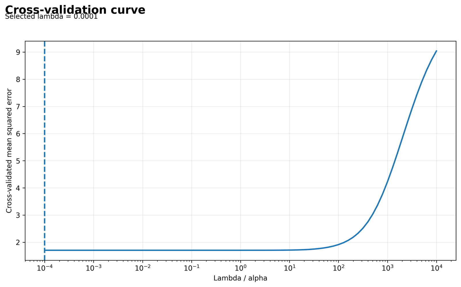
Validation error is lowest at the far-left candidate and remains relatively flat across weak penalties before rising under stronger shrinkage.
Selected lambda = 0.0001, mean CV MSE = 1.702748 and reported fold standard deviation = 1.008144.
The declared minimum-error rule finds no predictive benefit from visible shrinkage within the tested grid.
A boundary optimum must be reported honestly. Moving the line to a stronger penalty would change the verified model.
Python Chart 2: Coefficient Paths Across Lambda
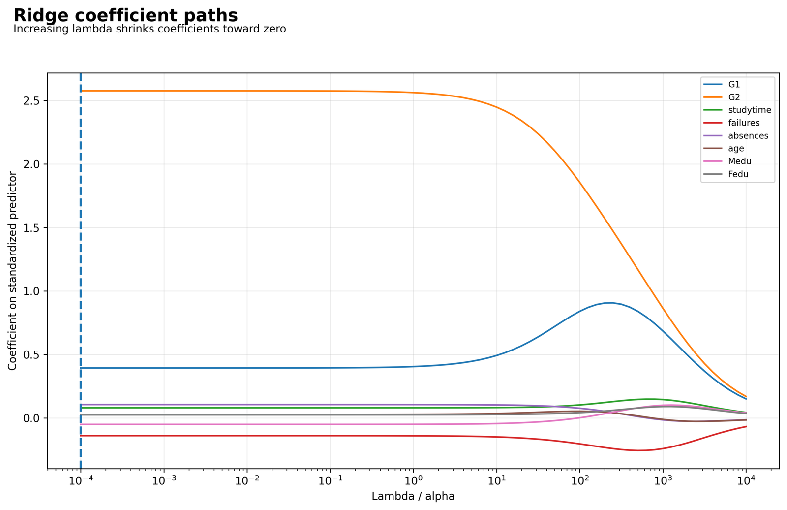
All eight slopes contract smoothly toward zero. No predictor is forced to an exact zero value.
At lambda 0.0001, G2 = 0.797368, G1 = 0.121758 and failures = −0.043185.
The graph shows redistribution of shared predictive information as regularization increases, especially for correlated grade predictors.
The path distinguishes Ridge Regression from lasso and shows how strongly an alternative lambda would alter the equation.
Python Chart 3: Selected Standardized Coefficients
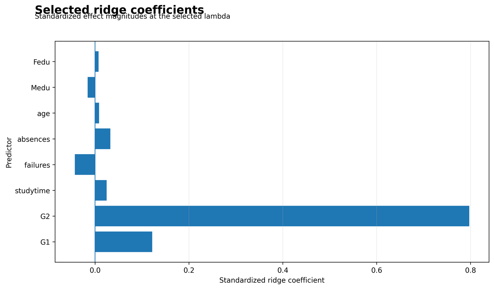
G2 dominates the equation, G1 is a distant second and the remaining absolute slopes are below approximately 0.05.
G2 = 0.797368, G1 = 0.121758, failures = −0.043185, absences = 0.032672 and studytime = 0.024792.
Standardized slopes compare conditional fitted movement on common predictor scales. They are not percentages of importance.
The chart identifies the dominant predictive direction while preserving the full eight-variable equation.
Python Chart 4: Observed versus Predicted Test Values
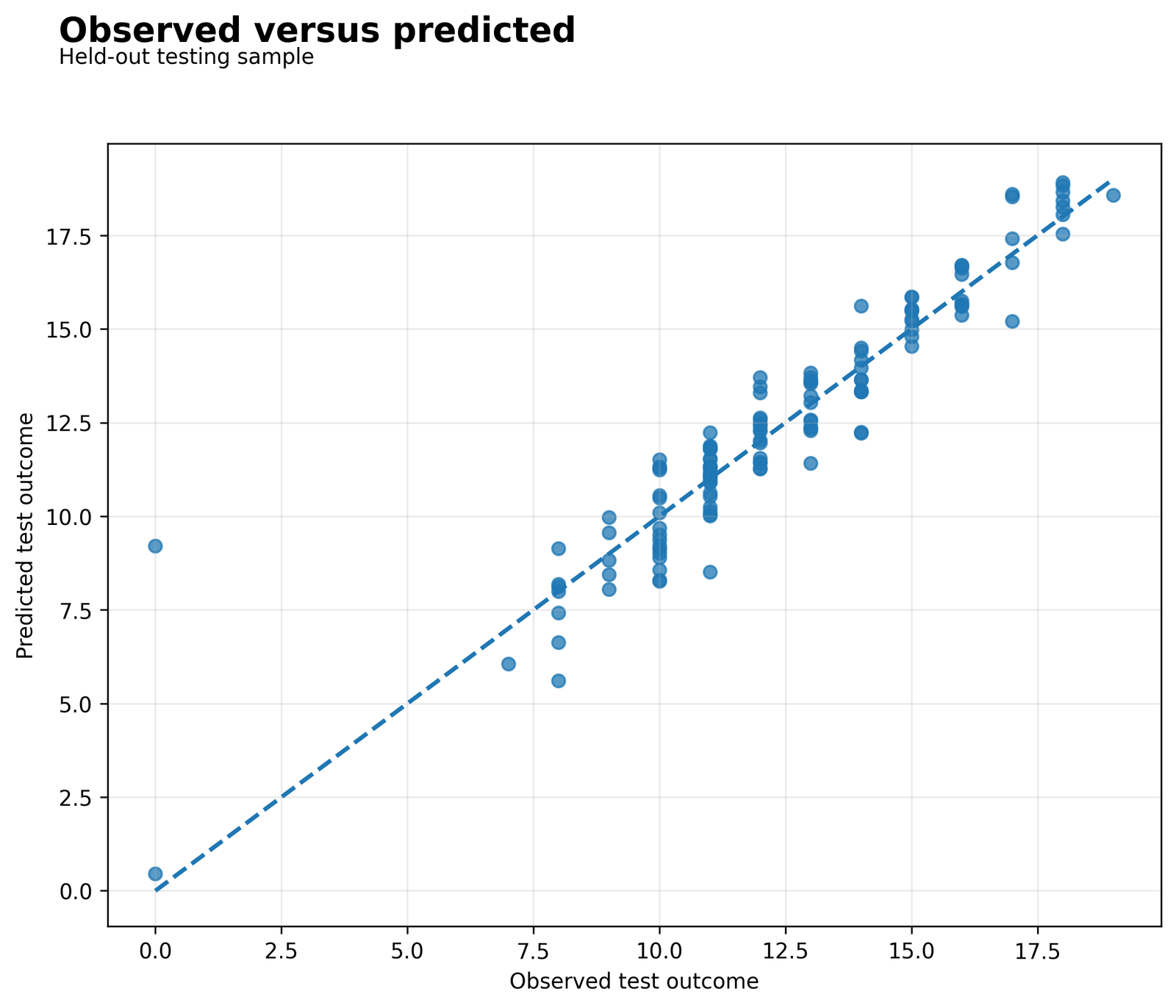
Most held-out observations follow the diagonal through the central grade range, while a smaller number of extreme outcomes have larger vertical errors.
Testing R² = 0.861117, RMSE = 1.163763 and MAE = 0.739991.
The figure evaluates unseen records from one fixed split and is more relevant to generalization than the final all-case refit.
Strong overall alignment does not guarantee accurate prediction for every student or transport to another cohort.
Python Chart 5: Test Residuals versus Predicted Values
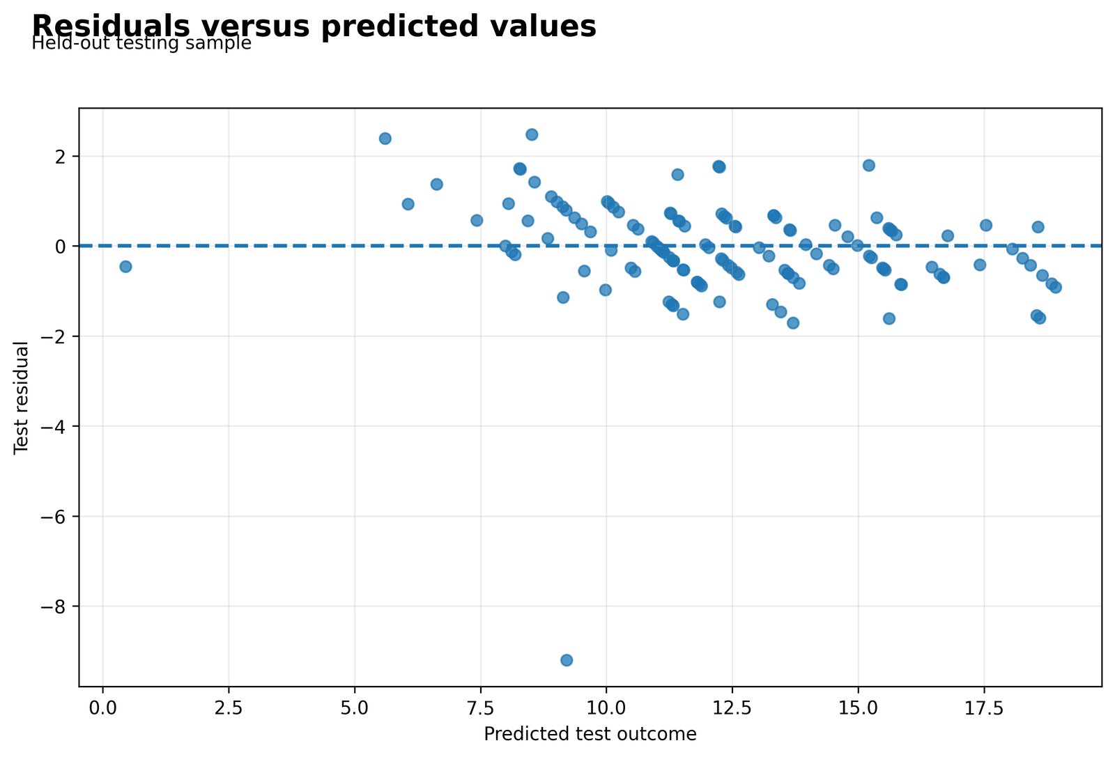
Residuals are broadly centered, integer grades create diagonal bands and several cases remain harder to predict.
Test RMSE exceeds MAE by approximately 0.423772 because larger errors receive greater squared-error weight.
L2 shrinkage controls coefficient magnitude but does not guarantee linearity, constant spread or symmetric errors.
The plot checks the complete fitted pipeline rather than only the coefficient vector.
Python Chart 6: Test Residual Distribution
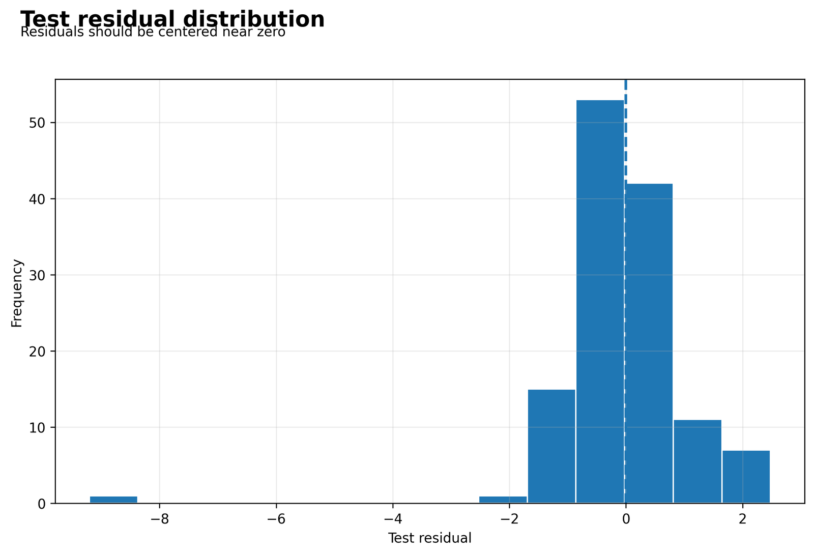
Most errors cluster near zero, while a smaller number of larger misses extend the tails.
RMSE = 1.163763 and MAE = 0.739991 summarize the same residuals with different sensitivity to large errors.
Regularization does not force prediction errors to be normal or remove grade-boundary effects.
The histogram reveals whether an acceptable average error hides a small group of difficult cases.
R Charts and Paired Explanations
The R evidence independently cross-checks the Ridge Regression calculations. The available R assets are arranged in two matched pairs, with one software-results card used where the supplied post does not contain a fourth unique R chart.
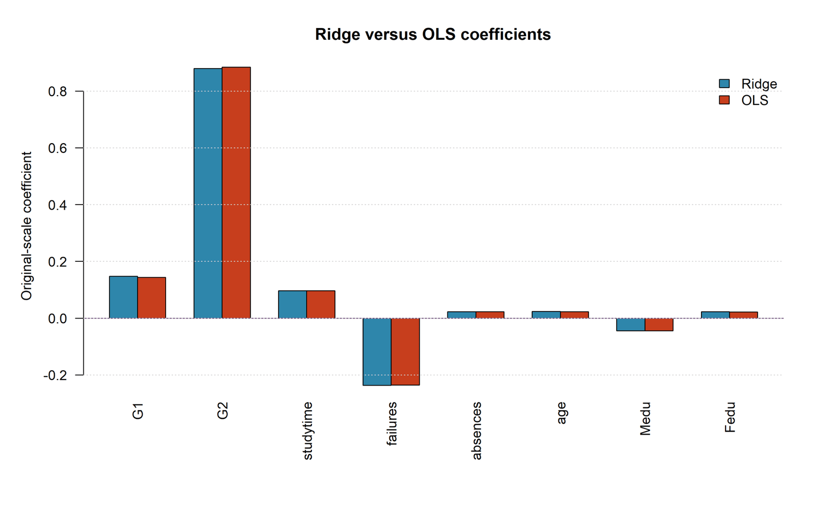
R Chart 1: Ridge versus OLS Coefficients
Pattern: The R penalty of 1 creates visible but modest displacement from OLS.
Key values: R coefficients include approximately G1 = 0.147402 and G2 = 0.879975, compared with OLS anchors 0.143397 and 0.884807.
Interpretation: Different penalty conventions and a different split create more shrinkage than the Python lambda 0.0001 result.
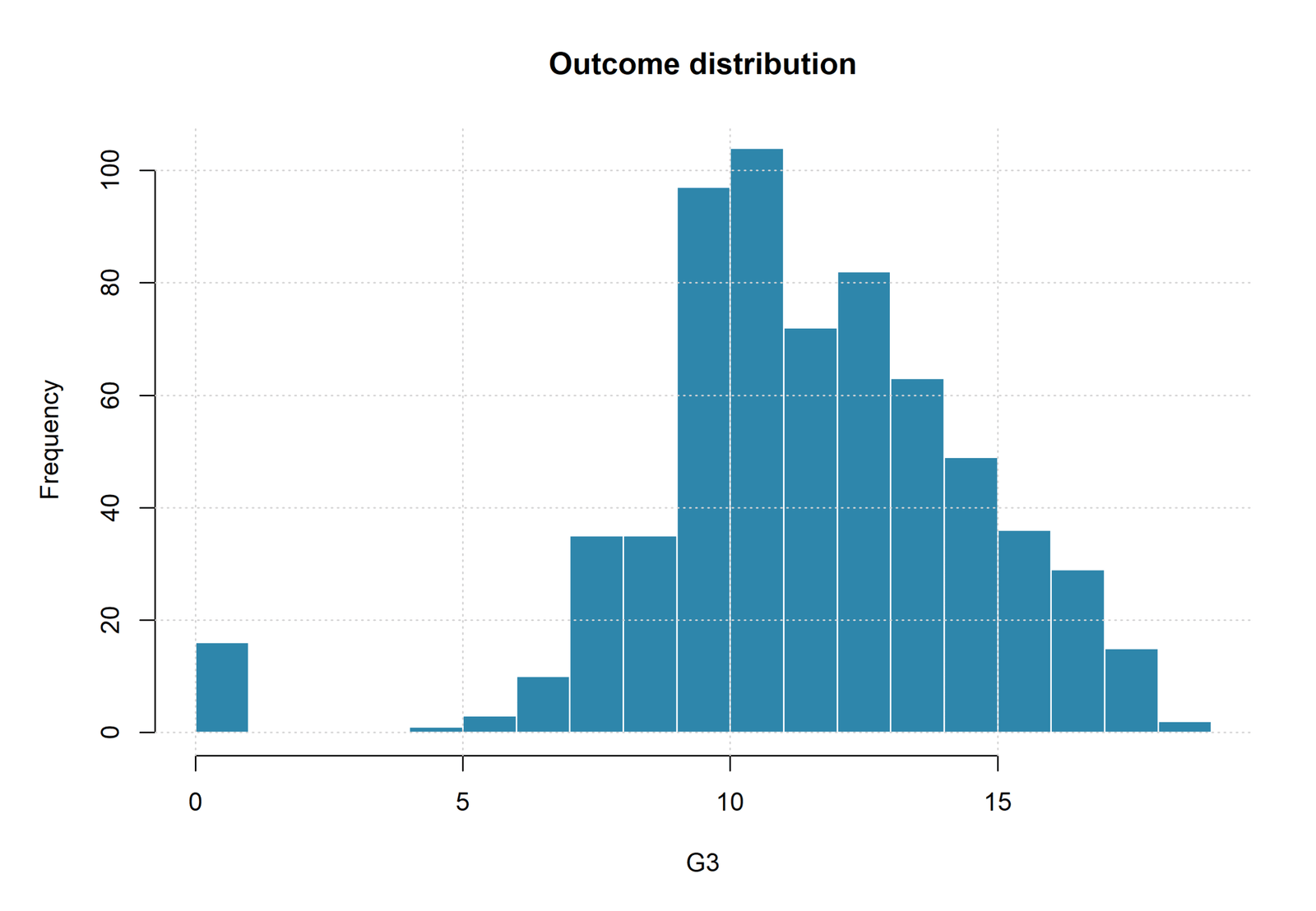
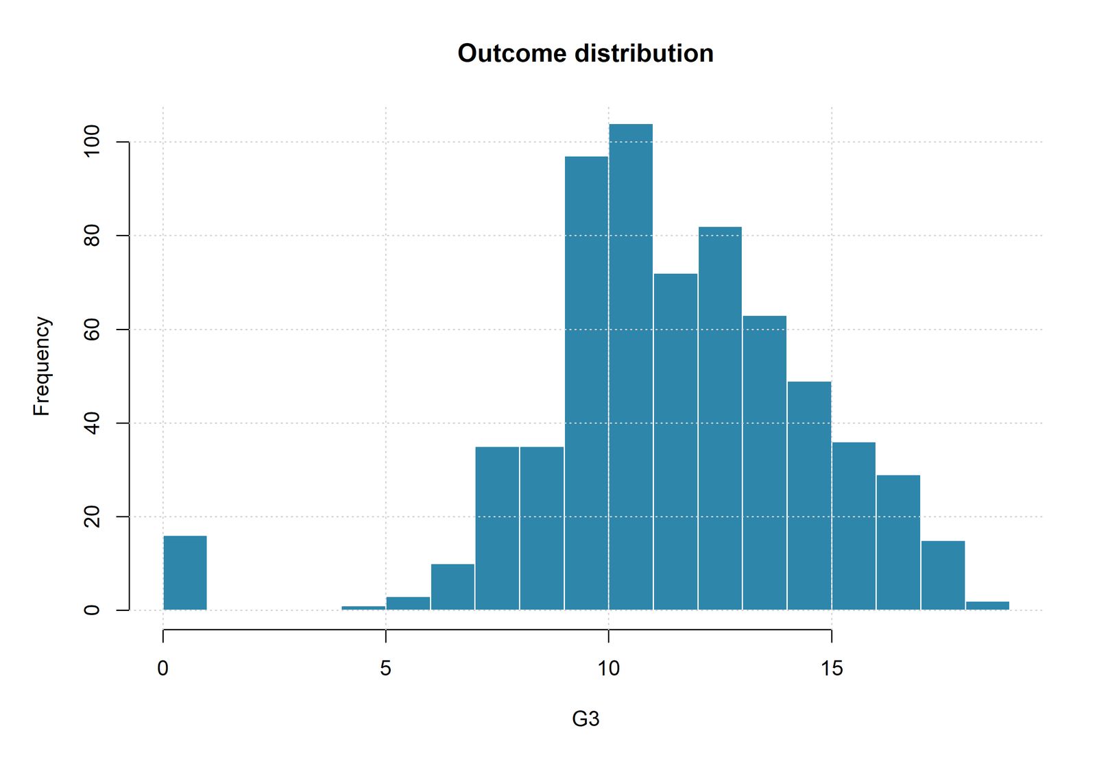
R Chart 2: Outcome Distribution
Pattern: G3 is integer-valued, concentrated in the middle range and includes low boundary outcomes.
Key values: The complete analysis contains 649 observations, while the R test partition contains 129.
Interpretation: Ridge predicts a continuous conditional mean and can miss some boundary outcomes substantially.
R Validation Summary
- Training n = 520
- Testing n = 129
- Selected lambda = 1
- Training R² = 0.835746
- Testing R² = 0.913199
- Testing RMSE = 0.915496
- Testing MAE = 0.746641
R Chart 3: Distribution Cross-Check
Pattern: The second R output asset confirms the same bounded and discrete outcome context.
Key values: Full-data R ridge R² = 0.850773, compared with full-data OLS R² = 0.850777.
Interpretation: The nearly identical fitted R² supports the conclusion that regularization produces little full-sample fit change.
R Evidence 4: Independent Holdout
Pattern: The R holdout produces stronger R² and lower RMSE than the Python holdout.
Key values: Testing R² = 0.913199, RMSE = 0.915496 and MAE = 0.746641.
Interpretation: Different case difficulty and partition membership can explain the difference.
Ridge Regression Coefficient and Parameter Interpretation
Primary Original-Scale Equation
Each coefficient is a partial predictive association under the selected Ridge Regression pipeline. Students differing by one point in G2 but equal on the other seven predictors differ by approximately 0.884807 points in fitted G3.
G2 has the largest standardized slope, 0.797368, and G1 is second at 0.121758. The remaining absolute standardized values are small. Coefficient magnitude depends on the feature set, scaling and penalty and should not be treated as a causal-importance ranking.
Failures has the largest negative standardized slope at −0.043185. Absences has a small positive adjusted slope of 0.022762 in original units. These signs describe the conditional fitted equation and do not establish beneficial or harmful interventions.
The coefficient differences from OLS are measured in millionths because lambda is 0.0001. The model therefore provides a regularized stability check rather than a substantially altered equation.
Predictions, Effects and Model Meaning
A Ridge Regression prediction is obtained by substituting identically defined predictor values into the original-scale equation. For the first supplied case—G1 = 0, G2 = 11, studytime = 2, failures = 0, absences = 4, age = 18, Medu = 4 and Fedu = 4—the full-precision fitted value is approximately 9.83267.
The observed G3 for that case is 11, so the observed-minus-predicted residual is approximately 1.16733. The downloadable case-evidence CSV preserves full-precision predictions and OLS comparisons.
A new case can also be scored in standardized space, but the stored training means and standard deviations must be reused. Recomputing scaling from one case or a new scoring batch changes the model.
Ridge Regression Assumptions and Diagnostics
Ridge Regression still assumes that the selected linear features adequately represent the conditional mean.
Scaling, fitting and lambda selection must occur without access to the final test outcomes.
Independent records and stable future feature definitions remain necessary for transport.
Residual Shape
The held-out residual-versus-predicted and residual-distribution charts show integer bands and a minority of larger misses. Regularization does not guarantee normality, homoscedasticity or a correct linear mean function.
Prediction Error
Test RMSE = 1.163763 and MAE = 0.739991. The difference shows that larger residuals materially affect squared error. Both metrics should be reported because they answer different loss questions.
Coefficient Stability
Traditional multicollinearity diagnostics remain useful for describing the original design, but Ridge Regression directly addresses coefficient instability through the L2 penalty. Stability should also be checked across folds, random splits and reasonable grids.
Test-Set Integrity
The testing partition provides a one-time evaluation. Any feature, transformation or lambda change motivated by the test residuals requires a new untouched evaluation sample.
Case-Level Review
The complete supplied source contains 330 preserved case rows with partition labels, ridge predictions, residuals, squared residuals and OLS comparisons. These records support auditing without printing a giant public HTML table.
Ridge Regression in Python, R, SPSS and Excel
Python
Python uses a Pipeline containing StandardScaler and Ridge, with GridSearchCV evaluating the 81-candidate grid.
- Training n = 519
- Testing n = 130
- Selected lambda = 0.0001
- Testing RMSE = 1.163763
R
R uses the same outcome and predictors through an independent glmnet workflow.
- Training n = 520
- Testing n = 129
- Selected lambda = 1
- Testing RMSE = 0.915496
SPSS
The supplied SPSS PDF preserves a software-specific analysis and auditing path. Penalized-regression availability depends on version and installed extensions.
- Verify the estimator and penalty settings.
- Audit the supplied equation through computed predictions.
- Run OLS on identical rows as a benchmark.
Excel
The workbook exposes model summaries, coefficient paths, candidate values and an original-scale prediction calculator.
- Use full-precision coefficients.
- Preserve training means and standard deviations.
- Calculate metrics within the declared partition.
Code and Formula Panels
Python leakage-safe Ridge Regression pipeline
from pathlib import Path

import numpy as np
import pandas as pd
from sklearn.linear_model import LinearRegression, Ridge
from sklearn.metrics import mean_absolute_error, mean_squared_error, r2_score
from sklearn.model_selection import GridSearchCV, KFold, train_test_split
from sklearn.pipeline import Pipeline
from sklearn.preprocessing import StandardScaler

DATA = Path("dataset.csv")
OUTCOME = "G3"
PREDICTORS = [
    "G1", "G2", "studytime", "failures",
    "absences", "age", "Medu", "Fedu"
]

# Replace with the archived seed used by the supplied analysis
# when exact 519/130 membership must be reproduced.
ARCHIVED_SEED = 12345

raw = pd.read_csv(DATA)
model_data = raw[[OUTCOME] + PREDICTORS].dropna().copy()

X = model_data[PREDICTORS].astype(float)
y = model_data[OUTCOME].astype(float)

X_train, X_test, y_train, y_test = train_test_split(
    X,
    y,
    test_size=130,
    random_state=ARCHIVED_SEED,
)

alpha_grid = np.logspace(-4, 4, 81)

pipeline = Pipeline([
    ("scale", StandardScaler()),
    ("ridge", Ridge(fit_intercept=True)),
])

cv = KFold(
    n_splits=10,
    shuffle=True,
    random_state=ARCHIVED_SEED,
)

search = GridSearchCV(
    estimator=pipeline,
    param_grid={"ridge__alpha": alpha_grid},
    scoring="neg_mean_squared_error",
    cv=cv,
    return_train_score=True,
    n_jobs=-1,
)

search.fit(X_train, y_train)
selected_alpha = float(search.best_params_["ridge__alpha"])

train_pred = search.predict(X_train)
test_pred = search.predict(X_test)

metrics = pd.DataFrame([
    {
        "partition": "training",
        "n": len(y_train),
        "r_squared": r2_score(y_train, train_pred),
        "rmse": mean_squared_error(y_train, train_pred) ** 0.5,
        "mae": mean_absolute_error(y_train, train_pred),
    },
    {
        "partition": "testing",
        "n": len(y_test),
        "r_squared": r2_score(y_test, test_pred),
        "rmse": mean_squared_error(y_test, test_pred) ** 0.5,
        "mae": mean_absolute_error(y_test, test_pred),
    },
])

# Final descriptive refit after tuning decisions are frozen.
final_pipeline = Pipeline([
    ("scale", StandardScaler()),
    ("ridge", Ridge(alpha=selected_alpha, fit_intercept=True)),
])
final_pipeline.fit(X, y)

scaler = final_pipeline.named_steps["scale"]
ridge = final_pipeline.named_steps["ridge"]

standardized_coef = ridge.coef_
original_coef = standardized_coef / scaler.scale_
original_intercept = (
    ridge.intercept_
    - np.sum(standardized_coef * scaler.mean_ / scaler.scale_)
)

ridge_coef = pd.DataFrame({
    "term": PREDICTORS,
    "ridge_standardized": standardized_coef,
    "ridge_original_scale": original_coef,
})

# OLS comparison on the same complete rows.
ols = LinearRegression().fit(X, y)
ridge_coef["ols_original_scale"] = ols.coef_
ridge_coef["ridge_minus_ols"] = (
    ridge_coef["ridge_original_scale"]
    - ridge_coef["ols_original_scale"]
)

final_pred = final_pipeline.predict(X)
ols_pred = ols.predict(X)

full_metrics = pd.DataFrame([
    {
        "model": "full-data ridge",
        "alpha": selected_alpha,
        "r_squared": r2_score(y, final_pred),
        "rmse": mean_squared_error(y, final_pred) ** 0.5,
        "mae": mean_absolute_error(y, final_pred),
    },
    {
        "model": "full-data OLS",
        "alpha": 0.0,
        "r_squared": r2_score(y, ols_pred),
        "rmse": mean_squared_error(y, ols_pred) ** 0.5,
        "mae": mean_absolute_error(y, ols_pred),
    },
])

cv_results = pd.DataFrame(search.cv_results_)
cv_export = pd.DataFrame({
    "alpha": cv_results["param_ridge__alpha"].astype(float),
    "mean_cv_mse": -cv_results["mean_test_score"],
    "sd_cv_mse": cv_results["std_test_score"],
    "mean_training_mse": -cv_results["mean_train_score"],
})

metrics.to_csv("ridge_train_test_metrics.csv", index=False)
full_metrics.to_csv("ridge_full_data_metrics.csv", index=False)
ridge_coef.to_csv("ridge_coefficients.csv", index=False)
cv_export.to_csv("ridge_cross_validation.csv", index=False)

print("Selected alpha:", selected_alpha)
print(metrics.to_string(index=False))
print(full_metrics.to_string(index=False))
print("Original-scale intercept:", original_intercept)
print(ridge_coef.to_string(index=False))
Exact supplied split results require the archived random seed and row membership. The code shows the verified workflow order and complete export logic.
R glmnet Ridge Regression workflow
library(glmnet)

dat <- read.csv("dataset.csv", check.names = FALSE)

outcome <- "G3"
predictors <- c(
  "G1", "G2", "studytime", "failures",
  "absences", "age", "Medu", "Fedu"
)

model_dat <- dat[
  complete.cases(dat[c(outcome, predictors)]),
  c(outcome, predictors)
]

x <- as.matrix(model_dat[predictors])
y <- model_dat[[outcome]]

# Replace with the archived seed when the exact supplied
# 520/129 partition must be reproduced.
set.seed(12345)
train_id <- sample(seq_len(nrow(model_dat)), size = 520)
test_id <- setdiff(seq_len(nrow(model_dat)), train_id)

lambda_grid <- 10 ^ seq(-4, 4, length.out = 81)

set.seed(12345)
cv_fit <- cv.glmnet(
  x = x[train_id, , drop = FALSE],
  y = y[train_id],
  alpha = 0,
  lambda = lambda_grid,
  nfolds = 10,
  standardize = TRUE,
  intercept = TRUE,
  type.measure = "mse"
)

lambda_selected <- cv_fit$lambda.min

train_pred <- as.numeric(
  predict(cv_fit, newx = x[train_id, , drop = FALSE],
          s = lambda_selected)
)
test_pred <- as.numeric(
  predict(cv_fit, newx = x[test_id, , drop = FALSE],
          s = lambda_selected)
)

metric_row <- function(actual, predicted, partition) {
  data.frame(
    partition = partition,
    n = length(actual),
    r_squared = 1 - sum((actual - predicted)^2) /
      sum((actual - mean(actual))^2),
    rmse = sqrt(mean((actual - predicted)^2)),
    mae = mean(abs(actual - predicted))
  )
}

metrics <- rbind(
  metric_row(y[train_id], train_pred, "training"),
  metric_row(y[test_id], test_pred, "testing")
)

# Final full-data ridge fit using the selected lambda.
final_fit <- glmnet(
  x = x,
  y = y,
  alpha = 0,
  lambda = lambda_selected,
  standardize = TRUE,
  intercept = TRUE
)

final_pred <- as.numeric(
  predict(final_fit, newx = x, s = lambda_selected)
)

full_metrics <- data.frame(
  model = "full-data ridge",
  lambda = lambda_selected,
  n = length(y),
  r_squared = 1 - sum((y - final_pred)^2) /
    sum((y - mean(y))^2),
  rmse = sqrt(mean((y - final_pred)^2)),
  mae = mean(abs(y - final_pred))
)

coef_table <- as.matrix(coef(final_fit, s = lambda_selected))
coef_export <- data.frame(
  term = rownames(coef_table),
  coefficient = as.numeric(coef_table[, 1]),
  row.names = NULL
)

write.csv(metrics, "ridge_r_train_test_metrics.csv", row.names = FALSE)
write.csv(full_metrics, "ridge_r_full_metrics.csv", row.names = FALSE)
write.csv(coef_export, "ridge_r_coefficients.csv", row.names = FALSE)

print(lambda_selected)
print(metrics)
print(full_metrics)
print(coef_export)
The R workflow is intentionally separate. Replacing the placeholder seed with the archived R seed is required to reproduce the supplied 520/129 membership exactly.
SPSS prediction and residual audit syntax
* SPSS audit of the verified original-scale ridge equation.
* This syntax audits predictions and residuals; it does not claim
* to refit the cross-validated penalized model in every SPSS edition.

COMPUTE ridge_pred =
 -0.501155
 + 0.143397 * G1
 + 0.884807 * G2
 + 0.096632 * studytime
 - 0.235361 * failures
 + 0.022762 * absences
 + 0.022686 * age
 - 0.044951 * Medu
 + 0.022025 * Fedu.

COMPUTE ridge_resid = G3 - ridge_pred.
COMPUTE ridge_sq_resid = ridge_resid ** 2.
COMPUTE ridge_abs_resid = ABS(ridge_resid).
EXECUTE.

DESCRIPTIVES VARIABLES=
 G3 ridge_pred ridge_resid ridge_sq_resid ridge_abs_resid
 /STATISTICS=MEAN STDDEV MIN MAX.

GRAPH
 /SCATTERPLOT(BIVAR)=ridge_pred WITH G3
 /TITLE='Ridge Regression: Observed and Predicted G3'.

GRAPH
 /SCATTERPLOT(BIVAR)=ridge_pred WITH ridge_resid
 /TITLE='Ridge Regression: Residuals and Predictions'.

GRAPH
 /HISTOGRAM(NORMAL)=ridge_resid
 /TITLE='Ridge Regression: Residual Distribution'.

* Run ordinary least squares on the same rows for comparison.
REGRESSION
 /MISSING LISTWISE
 /STATISTICS COEFF OUTS R ANOVA CI(95) COLLIN TOL
 /DEPENDENT G3
 /METHOD=ENTER G1 G2 studytime failures absences age Medu Fedu.

* Read the supplied SPSS output for the installed penalized-regression
* procedure and penalty configuration. Command availability varies
* by SPSS version and installed extensions.
This syntax audits the supplied final ridge equation and compares it with OLS. It does not invent a universal SPSS penalized-regression command.
Excel formulas for prediction and metric auditing
Workbook audit formulas

1. Original-scale ridge prediction
=Intercept
 +SUMPRODUCT(PredictorValueRange,CoefficientRange)

2. Row residual
=ObservedG3-PredictedG3

3. Squared residual
=ResidualCell^2

4. Absolute residual
=ABS(ResidualCell)

5. RMSE for a fixed evaluation partition
=SQRT(AVERAGE(SquaredResidualRange))

6. MAE for a fixed evaluation partition
=AVERAGE(AbsoluteResidualRange)

7. R-squared for a fixed evaluation partition
=1-SUM(SquaredResidualRange)/
 SUMXMY2(ObservedRange,AVERAGE(ObservedRange))

8. Standardize a new predictor with stored training values
=(RawValue-TrainingMean)/TrainingSD

9. Standardized-space prediction
=TrainingOutcomeMean
 +SUMPRODUCT(StandardizedInputRange,StandardizedCoefficientRange)

Important:
- Use the stored training means and standard deviations.
- Do not recalculate scaling from one new case.
- Do not use the test set to choose lambda.
- The workbook audits the fitted pipeline; it does not replace
  leakage-safe cross-validation unless all folds are implemented.
Use full-precision workbook coefficients for exact reproduction. Rounded article values are for communication.
Advanced Ridge Regression Topics
These 26 panels extend the worked analysis from basic L2 calculation to tuning uncertainty, coefficient interpretation, validation, deployment and responsible cross-software reporting.
1. Ridge Regression Estimand and Research Question
Ridge Regression estimates the coefficient vector that minimizes squared prediction error plus a declared L2 penalty. The target is not a model after correlated predictors are deleted. It is the penalized linear prediction rule defined by the outcome, feature matrix, scaling convention and selected lambda.
State whether the primary purpose is prediction, coefficient stabilization or a sensitivity comparison with ordinary least squares. A clear objective prevents a weakly penalized result from being described as a major regularization gain merely because Ridge Regression was used.
2. L2 Penalty Geometry
The L2 penalty constrains the squared length of the standardized slope vector. Geometrically, the least-squares contours meet a rounded constraint surface, so correlated coefficients tend to be reduced together rather than forcing one member of the group to zero.
This grouped behavior is one reason Ridge Regression can be more stable than lasso when G1 and G2 contain overlapping grade information. The exact coefficient allocation still depends on the sample and lambda.
3. Training-Fold Standardization
Predictor means and standard deviations must be estimated inside each training fold. The corresponding validation fold is transformed with those training-only values. This rule applies again when missing-value imputation or other learned preprocessing is added.
Scaling all 649 rows before cross-validation would allow validation observations to influence the transformation. The leakage may be numerically small, but the workflow would no longer provide a clean estimate of the complete Ridge Regression pipeline.
4. Intercept Treatment
The intercept is normally excluded from the penalty. Penalizing it would make predictions depend on the arbitrary zero point of the outcome and predictor coding rather than only on slope complexity.
When software centers the outcome and predictors internally, the reported intercept is reconstructed after the penalized slopes are estimated. Cross-software checks should confirm the intercept convention before comparing equations.
5. Candidate Lambda Grid
The Python workflow evaluates 81 candidates from 0.0001 through 10000. A logarithmic grid is appropriate because meaningful changes in shrinkage can occur across several orders of magnitude.
The grid is part of the analysis specification. Changing its lower or upper boundary after viewing the test result creates a new tuning analysis and requires the validation process to be repeated.
6. Minimum-Error Selection Rule
The supplied Python analysis chooses the candidate with the lowest mean ten-fold validation MSE. This rule selected lambda 0.0001 and therefore retained an almost ordinary-least-squares solution.
The minimum-error rule should not be replaced after viewing coefficient paths. A stronger penalty may be easier to illustrate, but it is not the verified selected model unless another rule was declared and rerun.
7. Boundary Optimum
The selected Python lambda is the smallest tested value. A boundary optimum means the available validation evidence prefers very weak shrinkage and does not identify an interior minimum within the grid.
The honest conclusion is that stronger Ridge Regression penalties were not rewarded under the supplied folds. A later grid may include smaller values or zero, but its result cannot be inferred from the current output.
8. One-Standard-Error Rule
A one-standard-error rule can select a simpler or more strongly penalized model whose mean validation loss remains within one estimated standard error of the minimum. It is a parsimony rule rather than the same rule as minimum error.
The exact fold-level uncertainty needed for a verified one-standard-error lambda is not supplied in the article. No alternative lambda should be invented from the plotted curve.
9. Fold Allocation and Random Seeds
Cross-validation results depend on which observations share a fold. A random seed, fold identifiers and split membership are therefore part of the reproducible Ridge Regression record.
A flat validation surface can allow nearby penalties to exchange rank when folds change. Reporting only the selected lambda without the fold design hides important tuning uncertainty.
10. Nested Cross-Validation
Nested cross-validation places lambda selection inside each outer training fold and evaluates the tuned pipeline on an outer validation fold. It estimates generalization while accounting for tuning variability.
One protected holdout is suitable for the worked example, but nested resampling is preferable when performance claims will guide consequential use or when several modeling choices are compared.
11. Test-Set Discipline
The 130 Python testing records should be opened only after the feature list, scaling process, grid, folds, scoring rule and selected lambda are fixed. Their outcomes must not guide a second round of tuning.
Changing predictors or lambda after seeing test RMSE converts the test set into another validation set. A new untouched sample would then be required for an unbiased final evaluation.
12. Coefficient Paths
A Ridge Regression coefficient path shows how standardized slopes change as lambda increases. Smooth contraction is expected because the L2 objective is continuous and normally retains every predictor.
Path crossings or changing relative magnitudes show how correlated predictors redistribute shared signal. They are not evidence that causal effects change with lambda.
13. Correlated Predictor Groups
G1 and G2 both measure prior academic performance. Ridge Regression can distribute predictive information across both variables rather than selecting one and discarding the other.
The individual slopes remain conditional on the full feature set. A stable prediction equation does not imply that each correlated coefficient has a uniquely determined scientific interpretation.
14. Standardized and Original-Scale Coefficients
Standardized coefficients describe the effect of a one-standard-deviation predictor change on the fitted outcome scale used by the model. They are useful for within-model magnitude comparison.
Original-scale coefficients are required for direct scoring with raw predictor values. Mixing raw values with standardized slopes produces invalid predictions.
15. Ordinary Least Squares Comparison
Ordinary least squares provides the unpenalized benchmark on the same 649 complete rows. At lambda 0.0001, the Python Ridge Regression coefficients differ from OLS only in approximately the sixth or seventh decimal place.
The near equality is a substantive result. It shows that the current validation design does not reward meaningful shrinkage, rather than proving that regularization is always unnecessary.
16. Python and R Lambda Conventions
Different libraries can scale the residual loss and penalty differently. The same printed numerical lambda may therefore produce different coefficient shrinkage.
Python and R also use different train-test partitions in the supplied evidence. Compare predictions, paths and complete workflow settings instead of treating lambda 0.0001 and lambda 1 as directly interchangeable numbers.
17. Effective Degrees of Freedom
Ridge Regression retains all eight predictors, but its effective model complexity declines continuously as lambda grows. Complexity is therefore not equal to the count of nonzero slopes.
Specialized effective-degrees-of-freedom calculations can support risk estimates and information criteria. They should be labeled clearly and should not be confused with the ordinary residual degrees of freedom from OLS.
18. Bias-Variance Trade-Off
Increasing lambda introduces bias by pulling coefficients toward zero. The potential benefit is lower variance across samples, especially when predictors overlap strongly.
The correct lambda balances these forces for the declared prediction loss. In this dataset, validation favors very little added bias because the eight-predictor OLS-like solution is already stable.
19. Prediction Intervals
The supplied files report point predictions and residual metrics, not validated individual prediction intervals. Classical OLS interval formulas do not automatically transfer to a tuned penalized pipeline.
Bootstrap or nested-resampling procedures can incorporate coefficient, tuning and residual uncertainty. The resampling design must reproduce every preprocessing and lambda-selection step.
20. Inference After Tuning
Classical p-values and confidence intervals should not be attached mechanically to selected Ridge Regression coefficients. Penalization and data-driven tuning change the sampling problem.
When inference is required, consider sample splitting, bootstrap methods or specialized penalized-inference procedures. Keep predictive estimation and confirmatory coefficient testing conceptually separate.
21. Missing Data
The worked model uses 649 complete observations. Complete-case fitting is transparent but assumes the omitted incomplete rows do not create serious selection bias for the intended use.
If imputation is introduced, it must occur inside each training fold. Ridge Regression is not a missing-data method, and robust prediction claims require the imputation process to be validated with the model.
22. Categorical Predictors
Categorical variables require a stable dummy-coding scheme with documented reference categories. Ridge can penalize the resulting indicator slopes, but the coding determines how coefficients and predictions are expressed.
When a multi-level factor is represented by several indicators, grouping or hierarchy considerations may matter. Standard ridge treats the individual columns according to their standardized scales.
23. Nonlinearity and Interactions
Ridge Regression remains linear in the supplied feature columns. It can penalize polynomial terms, splines and interactions, but those features must be created inside the validated pipeline.
Adding many nonlinear terms can make regularization more useful, yet the test set must remain protected while the expanded feature design and lambda are selected.
24. Outcome Timing and Information Availability
G2 is measured close to final G3 and therefore carries strong predictive information. A model intended for early intervention may not be allowed to use G2 because it is unavailable at the intended decision time.
Feature availability is part of model validity. High test R-squared does not make a temporally unavailable predictor suitable for deployment.
25. Deployment Monitoring
A deployed Ridge Regression model should be monitored for predictor drift, missingness, outcome calibration, subgroup error and changes in the residual distribution.
The original training means, standard deviations, feature order and coefficient precision must be versioned. Re-estimating scaling from each new batch changes the scoring system.
26. Ridge Regression Decision Framework
Begin with a clear prediction target and feature-availability rule. Preserve a transparent OLS benchmark, fit scaling and Ridge Regression inside cross-validation, select lambda by the declared loss and evaluate the test partition once.
Report the boundary optimum, split-specific metrics, coefficient paths, software differences and limitations. The defensible conclusion concerns validated predictive stability, not whether the method name sounds more advanced than OLS.
- Ridge Regression requires training-only preprocessing.
- Ridge Regression selects lambda from validation loss.
- Ridge Regression preserves the final test set.
- Ridge Regression reports boundary solutions openly.
- Ridge Regression keeps test and all-case metrics separate.
- Ridge Regression distinguishes standardized and raw-scale coefficients.
APA-Style Reporting
Worked Ridge Regression Report
An L2-penalized linear model predicted final grade G3 from G1, G2, studytime, failures, absences, age, maternal education and paternal education in 649 complete observations. The Python analysis used 519 training and 130 testing records. Predictor standardization was performed inside the modeling pipeline, and lambda was selected by minimum ten-fold cross-validated mean squared error from 81 candidates ranging from 0.0001 to 10000.
The selected lambda was 0.0001. On the protected testing records, R² was .861, RMSE was 1.164 and MAE was 0.740. The final all-case Ridge Regression refit had R² = .851 and RMSE = 1.247. Because the selected penalty was extremely weak, the original-scale ridge coefficients were nearly identical to ordinary least squares. G2 had the largest standardized coefficient, b = .797, followed by G1, b = .122.
A separate R workflow used 520 training and 129 testing records, selected lambda 1 and reported testing R² = .913, RMSE = .915 and MAE = .747. These results were reported separately because the held-out records and tuning process differed.
Publication Checklist
- State G3 as the continuous outcome.
- List all eight predictors in their fitted order.
- Report 649 complete observations.
- State the Python 519/130 split.
- State the independent R 520/129 split.
- Report the 81-value lambda grid.
- State that ten-fold CV selected 0.0001.
- Disclose that the optimum is at the lower boundary.
- Keep scaling inside every training fold.
- Protect the test outcomes from tuning.
- Report R², RMSE and MAE together.
- Keep test and all-case metrics separate.
- Report standardized and original-scale coefficients correctly.
- Do not attach ordinary OLS p-values to ridge coefficients.
- Keep Python and R holdout metrics separate.
- Verify all supplied chart and download URLs.
- Retain all five advertisement placements.
- Retain the fixed back-to-top control.
Downloads and Verification Resources
Ridge Regression R ReportIndependent split, selected lambda and validation evidence
Ridge Regression SPSS OutputSeparate SPSS software record and audit evidence
Worked Excel WorkbookModel summary, coefficient path and prediction calculator
Python Cross-Validation CurveMinimum-error lambda selection
Python Coefficient PathsL2 shrinkage across the candidate grid
Python Test PredictionsObserved versus predicted held-out values
R Ridge versus OLS CoefficientsIndependent coefficient cross-check
Frequently Asked Questions
What is Ridge Regression?
Ridge Regression is linear regression with an L2 penalty on standardized slopes. The penalty shrinks coefficients toward zero to improve stability while normally retaining every predictor.
What outcome and predictors were used?
Final grade G3 was predicted from G1, G2, studytime, failures, absences, age, Medu and Fedu in 649 complete observations.
What lambda did Python select?
Minimum ten-fold cross-validated MSE selected lambda 0.0001 from 81 candidates ranging from 0.0001 to 10000.
Why is the selected lambda so small?
The validation curve favored the least-penalized boundary. Stronger shrinkage increased the declared Python validation loss.
Does a small lambda mean Ridge Regression failed?
No. Tuning is allowed to select an almost unpenalized equation. It means the OLS-like solution predicted best among the tested candidates.
What were the Python test results?
For 130 protected testing records, R-squared was 0.861117, RMSE was 1.163763 and MAE was 0.739991.
Why are full-data ridge and OLS nearly identical?
Lambda 0.0001 produces extremely weak shrinkage. Their displayed full-data R-squared, RMSE and MAE are therefore the same.
Which predictor had the largest standardized coefficient?
G2 was largest at 0.797368, followed by G1 at 0.121758.
Does Ridge Regression remove predictors?
Usually no. L2 shrinkage keeps coefficients nonzero. Lasso is more appropriate when exact-zero selection is required.
Why standardize predictors?
The variables use different units. Standardization makes the common penalty act on comparable predictor scales and must be fitted from training data.
Should the intercept be penalized?
Normally no. The intercept represents the baseline location of the outcome and is usually excluded from the L2 penalty.
Can ordinary p-values be read from the ridge coefficients?
No. Classical OLS tests should not be copied onto tuned penalized coefficients without an appropriate inference procedure.
Why did R select lambda 1?
The R analysis used different training records, testing records, folds and library conventions. A relatively flat validation surface can produce different selected values.
Can the Python and R test metrics be averaged?
No. They describe different held-out observations and different tuned pipelines.
What should be done when the optimum is at the grid boundary?
Report the boundary result. A future analysis may expand the grid, but it must rerun cross-validation and preserve a new test strategy.
How should new data be scored?
Use the original-scale coefficient equation with identically defined raw inputs, or use the stored training means and standard deviations with standardized coefficients. Never recalculate scaling from one new case.
Ridge Regression Conclusion
The verified Python Ridge Regression workflow protects 130 testing records, fits scaling inside the training process and evaluates 81 lambda values through ten-fold cross-validation. The minimum validation error occurs at lambda 0.0001.
The Python testing records produce R² = 0.861117, RMSE = 1.163763 and MAE = 0.739991. The final 649-row ridge refit has R² = 0.850777 and RMSE = 1.247020, essentially identical to ordinary least squares because the selected penalty is extremely weak.
G2 remains the dominant standardized predictor, followed by G1. All eight predictors remain in the equation. The separate R workflow selects lambda 1 on a different split and therefore retains its own holdout metrics and coefficient comparison.
The defensible conclusion is not that Ridge Regression automatically outperforms OLS. It provides a transparent, leakage-safe regularization test and shows that this dataset favors an OLS-like prediction equation under the supplied Python validation design.

