Games–Howell in Python
with statsmodels 0.15
Welch ANOVA + Games–Howell Post Hoc Test — Complete Step-by-Step Guide
pairwise_tukeyhsd() now supports Games–Howell natively with use_var="unequal". The equal-variance Tukey path remains use_var="equal".What Is the Games–Howell Test?
Games–Howell is a post hoc multiple-comparison procedure for comparing all pairs of independent group means when a common within-group variance is not a good description of the data. It is often paired with Welch ANOVA because both methods allow the groups to contribute their own variance information instead of forcing every comparison to use one pooled error variance.
The practical problem is easy to see. Suppose four training groups have different sample sizes, and one group is much more variable than the others. A five-point difference between two stable groups is not the same evidential situation as a five-point difference involving the very noisy group. Tukey HSD, under its equal-variance model, relies on pooled within-group variation. Games–Howell instead builds a standard error for each pair from the two variances and sample sizes involved in that pair and uses Welch–Satterthwaite degrees of freedom.
That difference is not a minor implementation detail. In the worked dataset below, the same six raw mean differences are passed to Tukey and Games–Howell, yet two significance decisions reverse. Control versus Video is not significant under Tukey but is significant under Games–Howell. Video versus Interactive changes in the opposite direction. This is why the post hoc method should be selected from the variance structure and design rather than from whichever output produces the preferred p-value.
Games–Howell is not a nonparametric test, and it is not simply a “stricter Tukey.” It remains a parametric procedure for differences in means. It can produce a larger adjusted p-value than Tukey for a noisy pair, but it can also produce a smaller adjusted p-value for a precise pair when an unrelated high-variance group inflates the pooled error used by Tukey.
For a deeper method definition, use the existing Salar Cafe pages on Games–Howell, Welch’s ANOVA, and Tukey HSD. This page stays focused on the Python workflow and the new statsmodels 0.15 implementation.
When Should You Use Games–Howell?
The most useful decision is not “Which post hoc test is popular?” but “Which uncertainty model matches the study?” Start with the design. The observations must be independent for the workflow used here. If the same person contributes scores to several conditions, if students are clustered inside classes, or if measurements are repeated over time, neither Welch ANOVA nor Games–Howell repairs that dependence. You need a repeated-measures, mixed-effects, cluster-aware, or otherwise design-appropriate model.
Next inspect the actual scale of variance inequality. A significant Levene test can support the decision, but it should not become a gatekeeper. With a very large sample, tiny variance differences can generate small p-values. With small samples, meaningful heteroscedasticity may fail to reach a conventional threshold. Group standard deviations, sample sizes, raw plots, outliers, and the scientific meaning of the outcome provide context that a single p-value cannot.
| Situation | Omnibus test | Pairwise follow-up |
|---|---|---|
| Independent groups; equal variance is defensible | One-way ANOVA | Tukey HSD / Tukey–Kramer |
| Independent groups; variances differ materially | Welch ANOVA | Games–Howell |
| Only two independent groups; variances differ | Welch independent-samples t test | |
| Repeated or matched observations | Use a repeated-measures or mixed model instead | |
Unequal sample sizes alone do not automatically require Games–Howell. When variances are reasonably equal, Tukey–Kramer handles unequal group sizes within the equal-variance framework. The stronger reason for Games–Howell is the combination of unequal variances with a design in which pair-specific uncertainty matters.
The example below is deliberately useful for teaching because the variance pattern is extreme enough to make the consequence visible. Group n ranges from 18 to 35, while SD ranges from 3.81 to 13.09. The smallest high-variance group is Interactive, and the largest low-variance group is Tutoring. That imbalance makes a pooled error term a questionable description of every pair.
Finally, remember that Games–Howell answers pairwise questions about means. If the outcome is strongly ordinal, heavily censored, dominated by extreme outliers, or scientifically better described by a median, quantile, probability, or count model, the mean-comparison workflow itself may not be the correct target.
Deep dive: edge cases when the decision is not obvious
Real datasets are often less clear than the example. You may see a moderate variance ratio, nearly equal sample sizes, and a Levene p-value close to .05. In that situation, do not pretend the software can identify one uniquely correct path from a threshold. Instead, ask whether the equal-variance approximation materially changes the uncertainty that matters for the research question.
A useful sensitivity strategy is to run the standard and Welch omnibus tests and compare the conclusions without cherry-picking. If the two analyses agree strongly, the practical decision may be robust even though the assumptions are not perfect. If they differ, the variance structure deserves more attention. The same idea applies to Tukey and Games–Howell: comparing them can be educational, but the primary method should still be declared from the design and diagnostics rather than selected after seeing which pair becomes significant.
Small groups deserve particular caution. Games–Howell is designed for unequal variances, but pair-specific degrees of freedom can become low when a comparison includes a small, highly variable group. A very wide confidence interval is not a software failure; it is the analysis reflecting limited information. Adding more decimal places does not create precision that the design did not collect.
With extremely unbalanced designs, inspect which groups carry the largest variance. The most problematic pattern for a pooled-variance analysis is often when small groups have large variance and large groups have small variance, or the reverse. Equal-variance ANOVA can behave differently depending on how sample size and variance are associated. Welch is popular precisely because it is designed to reduce sensitivity to that combination.
Do not confuse variance heterogeneity with variance caused by a transformation problem. Sometimes a positive outcome has variability that increases naturally with its mean. A scientifically sensible transformation or a model with an appropriate mean–variance relationship may be better than treating heteroscedasticity as an isolated nuisance. The correct method depends on the measurement process, not only the output of a homogeneity test.
Finally, remember that “post hoc” does not mean “unplanned and unlimited.” Games–Howell is appropriate for a family of pairwise mean comparisons. If the study had a small number of pre-specified contrasts, a contrast-based model can answer those questions more directly and often with greater power. A good analysis begins from the research questions and uses an all-pairs post hoc procedure when all pairs are genuinely relevant.
Our Example Dataset
The downloadable dataset contains 101 independent observations from four training conditions. Each row represents one observation, group identifies the training condition, and score is the quantitative outcome. The data are synthetic so the tutorial can be redistributed and reproduced safely, but every number in the article is calculated from the saved CSV rather than typed into a mock output table.
| Variable | Role | Type | Meaning |
|---|---|---|---|
id | Identifier | String | Unique observation ID |
group | Independent variable | Categorical | Control, Video, Interactive, or Tutoring |
score | Dependent variable | Numeric | Post-training score |
Use a long-format dataframe because it makes the same grouping column available to descriptive summaries, Welch ANOVA, and the statsmodels multiple-comparison function. The first code block also fixes the intended group order so tables and figures do not silently switch to alphabetical order.
import pandas as pd

order = ["Control", "Video", "Interactive", "Tutoring"]

df = pd.read_csv("posthoc_training_scores.csv")
df["group"] = pd.Categorical(
    df["group"],
    categories=order,
    ordered=True,
)

print(df.head())
print("Rows:", len(df))
print(df["group"].value_counts(sort=False))Rows: 101 Control 20 Video 28 Interactive 18 Tutoring 35
Before continuing, confirm that the group labels are exactly the levels you expect, scores are numeric, and missing values are understood. Strings such as "Control" and "Control " are different values. A stray space can create an unexpected fifth level and therefore a different number of pairwise comparisons. Good statistical programming begins by making malformed input fail clearly rather than silently producing a plausible-looking table.
df["group"] = df["group"].astype("string").str.strip()

unexpected = set(df["group"].dropna()) - set(order)
if unexpected:
    raise ValueError(f"Unexpected groups: {unexpected}")

if df["score"].isna().any():
    raise ValueError("Resolve missing outcome values before analysis.")

if not pd.api.types.is_numeric_dtype(df["score"]):
raise TypeError("score must be numeric.")Descriptive Statistics
Descriptive statistics are not a decorative preface to the “real” test. They reveal the exact features that determine whether a pooled variance model is credible. Compute the group sample size, mean, standard deviation, standard error, median, and range before any ANOVA call.
import numpy as np

desc = (
    df.groupby("group", observed=True)["score"]
      .agg(
          n="count",
          mean="mean",
          sd="std",
          median="median",
          minimum="min",
          maximum="max",
      )
)

desc["se"] = desc["sd"] / np.sqrt(desc["n"])
print(desc.round(3))| Group | N | Mean | SD | SE | Median | Min | Max |
|---|---|---|---|---|---|---|---|
| Control | 20 | 71.75 | 4.54 | 1.02 | 71.0 | 60 | 81 |
| Video | 28 | 76.57 | 6.00 | 1.13 | 77.0 | 66 | 88 |
| Interactive | 18 | 82.22 | 13.09 | 3.08 | 82.5 | 55 | 100 |
| Tutoring | 35 | 83.23 | 3.81 | 0.64 | 83.0 | 74 | 91 |
The means rise from 71.75 in Control to 83.23 in Tutoring, so an overall mean difference is plausible. But the stronger diagnostic signal is the SD pattern. Interactive has SD 13.09, more than three times the Tutoring SD of 3.81, and Interactive also has the smallest sample size. Tutoring has the largest n and smallest SD, so its mean is estimated much more precisely.
This matters for post hoc inference. The Control–Video pair contains two relatively stable groups. The Video–Interactive pair contains one very noisy group. A procedure that uses the same pooled error variance for both pairs can represent one comparison better than the other. Games–Howell allows the pairwise standard error to respond to the actual two variances involved.
Visualizing the Data
Use plots that expose both location and spread. A mean-only bar chart would hide the most important feature of this dataset: the Interactive group is much more variable. The figures below were generated from the same CSV used in the calculations.
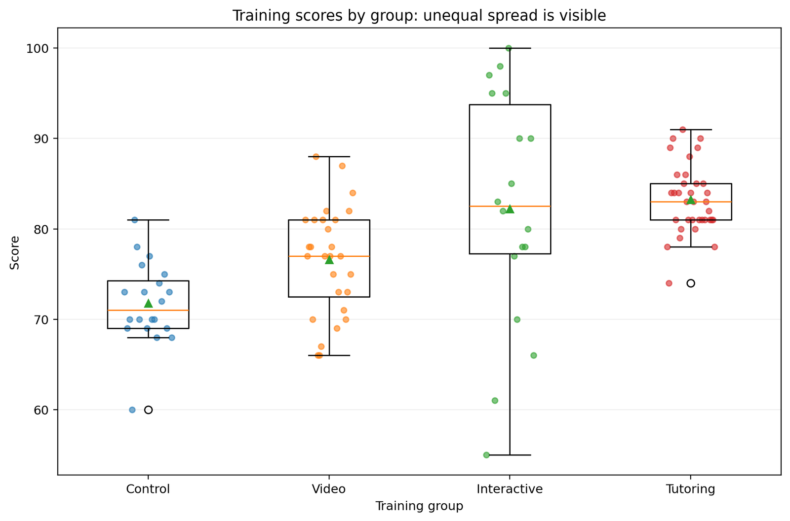
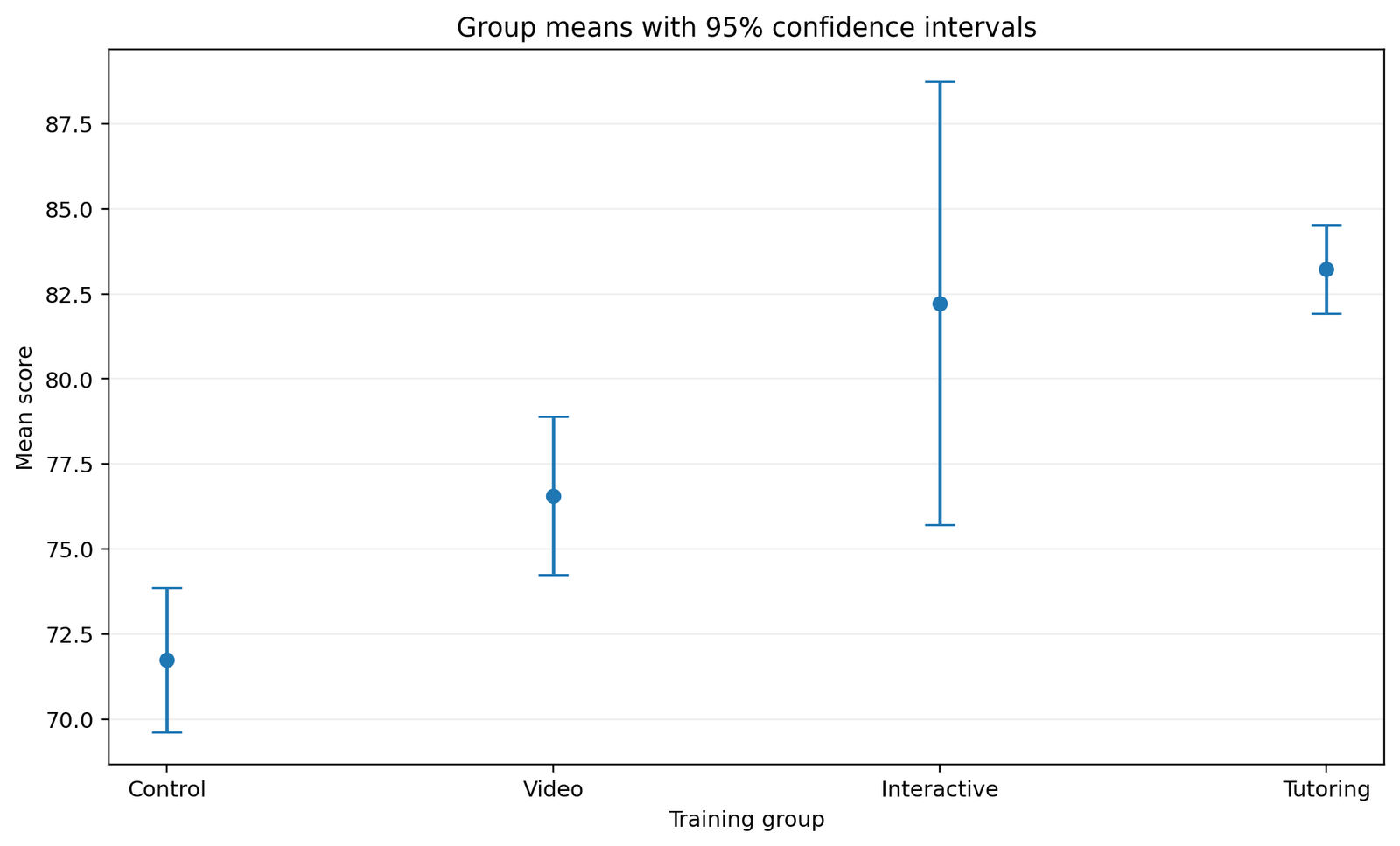
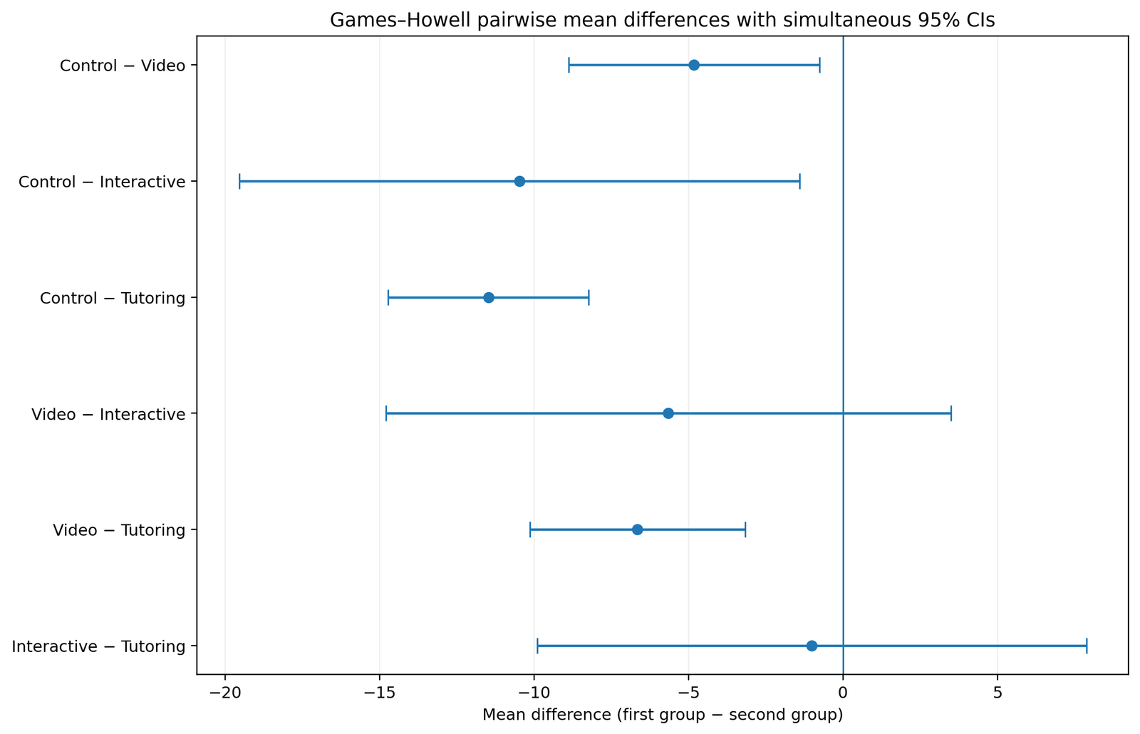
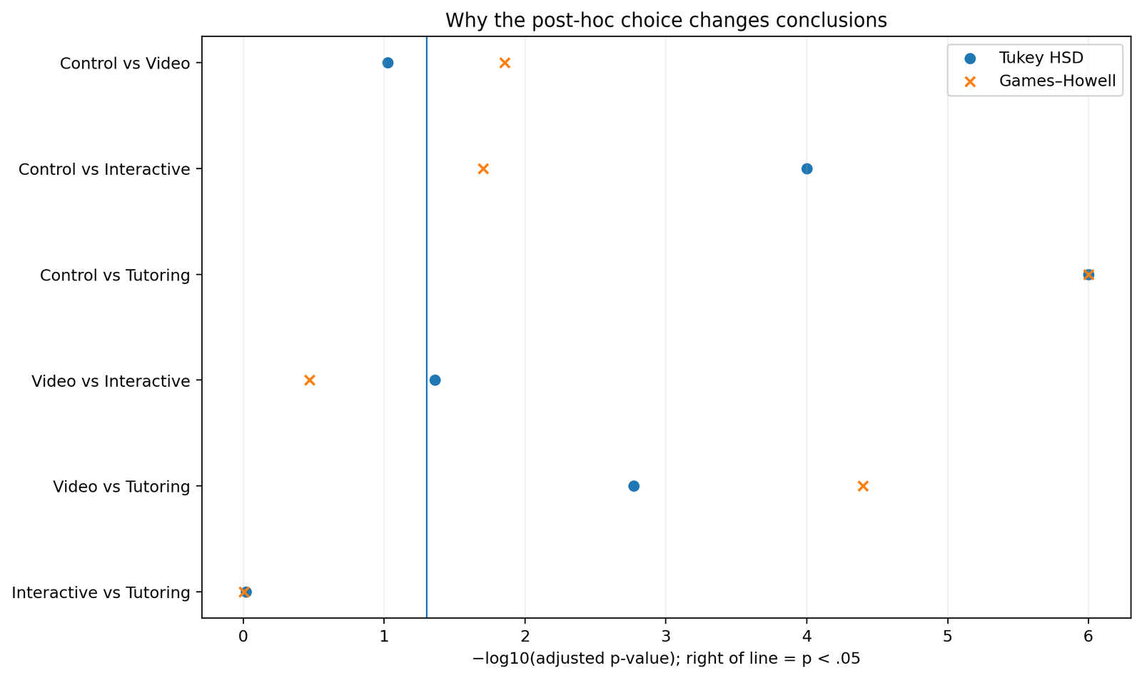
Figure 1 makes the variance problem visible before any formal test. Interactive spans a much wider score range than the other groups. Figure 2 shows the corresponding uncertainty in the group means: Interactive and Tutoring have similar high means, but the interval around Interactive is much wider. Do not use overlap between separate group-mean intervals as a substitute for a multiple-comparison test; they answer a different question.
Figures 3 and 4 become useful after the inferential steps. The Games–Howell forest plot shows the direction, magnitude, and simultaneous uncertainty for each difference. The comparison plot makes the two reversed Tukey/Games–Howell decisions visible immediately. A reader can therefore understand not only that the methods differ, but where the pooled and pair-specific variance models affect the conclusions.
Check Assumptions
The workflow has three distinct assumption questions: independence, variance structure, and whether mean-based inference is a sensible description of the outcome. The first is a property of the study design, not something Python can prove from the values alone. The second can be investigated with group SDs, plots, and a variance test. The third requires judgement about skewness, outliers, measurement scale, and the scientific target.
Median-centered Levene test
from scipy import stats

arrays = [
    df.loc[df["group"] == g, "score"].to_numpy()
    for g in order
]

levene_result = stats.levene(*arrays, center="median")
print(levene_result)H₀: all group variances are equal
F(3, 97) = 13.428, p < .001
Result: reject H₀. Variances are unequal → prefer Welch ANOVA + Games–Howell for this dataset.
Centering on the group median gives the Brown–Forsythe form of Levene’s test. It is generally less sensitive to non-normal observations than the original mean-centered version. Here the formal test is not operating in isolation: the SDs range from 3.81 to 13.09 and the raw plot shows a visibly wider Interactive group. The descriptive and formal evidence agree.
Normality and outliers
Do not turn normality testing into another binary ritual. With small groups, a formal normality test can have little power; with very large groups, trivial deviations can become statistically significant. Inspect raw distributions and Q–Q plots for strong curvature, heavy tails, floor or ceiling effects, and individual observations that dominate a group. A flagged outlier is not an automatic deletion. Remove a value only for a defensible reason such as a confirmed entry error or a pre-specified exclusion criterion.
import matplotlib.pyplot as plt
from scipy import stats

for g in order:
    x = df.loc[df["group"] == g, "score"].to_numpy()
    fig, ax = plt.subplots(figsize=(5, 4))
    stats.probplot(x, dist="norm", plot=ax)
    ax.set_title(f"Q–Q plot: {g}")
    plt.tight_layout()
    plt.show()
Welch and Games–Howell specifically address unequal variance. They do not make dependent observations independent and they do not guarantee robustness to every distributional problem. If the study has repeated measurements, clustering, or another dependence structure, use a model that represents that design.
Deep dive: diagnostics that are worth checking before you trust the result
Start with impossible values. If a score is defined on a 0–100 scale, values below 0 or above 100 should trigger a data-quality investigation before any statistical test. Range checks are simple and often catch errors that assumption tests cannot. Next check duplicates and identifiers. Repeated IDs may be legitimate repeated observations, accidental duplicate imports, or evidence that the independence assumption is wrong. The statistical consequence depends on why the duplicate exists.
Missing values require an explicit analysis rule. Calling dropna() is easy, but complete-case deletion is not automatically unbiased. If missingness differs by group or depends on the outcome, removing rows can change both the means and the variance pattern. Count missing values by group, document the reason for exclusion, and separate data cleaning from inferential decisions.
For outliers, combine numerical flags with the raw observations. The 1.5×IQR rule can identify cases worth checking, but it is not a universal deletion criterion. A legitimate extreme observation contains information about the population. Removing it because it makes Levene significant or changes a pairwise p-value is a form of outcome-driven analysis. If an observation is influential but valid, report a sensitivity analysis rather than silently deleting it.
Q–Q plots are useful because they show the direction and location of non-normality. Mild tail deviations in moderate samples are different from a tiny group with one extreme point. Mean-based methods can be robust in many ordinary situations, but robustness is not a license to ignore data structure. If the outcome is strongly skewed by construction, such as waiting time or cost, consider whether a transformation or a generalized model better represents the scientific process.
Independence is the assumption most likely to be misunderstood because there is no generic “independence test” that proves it from a column of scores. Independence comes from how observations were sampled and assigned. Students from the same classroom share context, repeated observations from the same participant share a subject, and neighboring spatial observations share location. Treating those rows as independent can make standard errors too small even if the variance test and normality plots look perfect.
For a public tutorial, it is helpful to state what the method does not solve. Welch addresses unequal group variances in an independent-groups mean comparison. Games–Howell addresses pairwise mean comparisons under that unequal-variance setting. Neither procedure automatically handles clustering, repeated measurements, covariates, multiple factors, informative missingness, or arbitrary distributional shapes. Those are separate modeling choices.
One-Way ANOVA (Equal Variances Assumed)
Run the conventional one-way ANOVA as a benchmark because it shows what the pooled equal-variance model would conclude. The omnibus null hypothesis is that all four population means are equal. A significant result means at least one differs; it does not imply that every pair is different.
from statsmodels.stats.oneway import anova_oneway

classic = anova_oneway(
    df["score"],
    df["group"],
    use_var="equal",
)

print(classic)| Source | df | F | p-value |
|---|---|---|---|
| Between groups | 3 | 13.757 | < .001 |
| Within groups | 97 | — | — |
The test is statistically significant, but the strong variance heterogeneity makes it a less defensible primary inference for this example. The pooled within-group error is influenced by all four groups. That is precisely what later creates a mismatch for some pairwise comparisons: the extremely variable Interactive group contributes to the common Tukey error even when a comparison involves only Control and Video.
It is useful to keep this result rather than delete it because comparing the standard and robust paths teaches a substantive lesson. Both omnibus tests reject equality, but their F statistics and denominator degrees of freedom differ because they estimate uncertainty differently. The post hoc section will show a more dramatic consequence: two pairwise decisions reverse.
Welch ANOVA
Welch ANOVA is the preferred omnibus analysis for this dataset because it does not require a common population variance. It gives greater influence to groups whose means are estimated precisely and less to groups with high variance relative to sample size.
welch = anova_oneway(
    df["score"],
    df["group"],
    use_var="unequal",
)

print(welch)H₀: the four population means are equal
F(3, 42.49) = 32.038, p < .001
Conclusion: at least one mean differs after allowing for unequal group variances.
The denominator degrees of freedom are fractional because Welch uses a Satterthwaite-type approximation based on the group variances and sample sizes. A useful conceptual weight is nᵢ / sᵢ². Tutoring has n = 35 and SD = 3.81, so its mean is estimated very precisely. Interactive has n = 18 and SD = 13.09, so it contributes much less precision. Welch allows that asymmetry to affect the omnibus statistic.
Welch ANOVA and Games–Howell form a coherent workflow: the omnibus test allows group-specific variances, and the pairwise procedure allows pair-specific variances and degrees of freedom. A common mistake is to run Welch because homogeneity is doubtful and then automatically use a standard pooled-variance Tukey test. That mixes two variance models in the same inferential chain.
The Welch result answers only the omnibus question. It tells us that the four means are not all equal, but not which pairs are supported. The next two sections deliberately run both Tukey and Games–Howell on the same observations so the consequence of the variance model can be seen directly.
Post Hoc: Tukey HSD
Tukey HSD is the standard all-pairs procedure under an equal-variance model. In statsmodels 0.15, request that path explicitly with use_var="equal". The function returns the mean difference, familywise-adjusted p-value, simultaneous confidence interval, and reject decision for each pair.
from statsmodels.stats.multicomp import pairwise_tukeyhsd

tukey = pairwise_tukeyhsd(
    endog=df["score"],
    groups=df["group"],
    alpha=0.05,
    use_var="equal",
)

tukey_table = tukey.summary_frame()
print(tukey_table)| Pair | Mean difference | Adjusted p | Decision |
|---|---|---|---|
| Control vs Video | 4.82 | .094 | Not significant |
| Control vs Interactive | 10.47 | < .001 | Significant |
| Control vs Tutoring | 11.48 | < .001 | Significant |
| Video vs Interactive | 5.65 | .044 | Significant |
| Video vs Tutoring | 6.66 | .002 | Significant |
| Interactive vs Tutoring | 1.01 | .960 | Not significant |
Under Tukey, four of the six pairs are significant. Control versus Video is not, even though the two groups individually have modest SDs. Video versus Interactive is just significant even though Interactive is the most variable group. Those two results are exactly the pairs to watch when we switch to Games–Howell.
Tukey is not “wrong” in the abstract. It answers the all-pairs question under a pooled equal-variance model. The issue is whether that model is a good representation of this dataset. Because the variance diagnostics strongly argue against a common variance, Tukey is included here as a comparison rather than the primary final post hoc analysis.
Post Hoc: Games–Howell in statsmodels 0.15
This is the software change that makes the page timely. In statsmodels 0.15, the same high-level function can run the unequal-variance Games–Howell procedure by setting use_var="unequal". There is no need to switch to a separate Python package merely to obtain the pairwise test.
games_howell = pairwise_tukeyhsd(
    endog=df["score"],
    groups=df["group"],
    alpha=0.05,
    use_var="unequal",
)

gh_table = games_howell.summary_frame()
print(gh_table)| Pair | Mean difference | Simultaneous 95% CI | Adjusted p | Decision |
|---|---|---|---|---|
| Control vs Video | -4.82 | -8.88 to -0.77 | .014 | Significant |
| Control vs Interactive | -10.47 | -19.54 to -1.41 | .020 | Significant |
| Control vs Tutoring | -11.48 | -14.73 to -8.23 | < .001 | Significant |
| Video vs Interactive | -5.65 | -14.79 to 3.49 | .338 | Not significant |
| Video vs Tutoring | -6.66 | -10.14 to -3.18 | < .001 | Significant |
| Interactive vs Tutoring | -1.01 | -9.89 to 7.88 | .988 | Not significant |
Again, four pairs are significant, but they are not the same four as Tukey. The pairwise intervals make the result easier to understand than a star column. Control versus Video has a simultaneous interval that excludes zero. Video versus Interactive has a wide interval that crosses zero because Interactive contributes substantial uncertainty.
Games–Howell calculates pair-specific uncertainty from sᵢ²/nᵢ + sⱼ²/nⱼ and uses a Welch–Satterthwaite degrees-of-freedom approximation for each pair. The comparison is then evaluated with Studentized-range logic to control the all-pairs family. That is why six unadjusted Welch t tests are not an equivalent replacement.
use_var="equal" → Tukey HSD; use_var="unequal" → Games–Howell.Deep dive: how the Games–Howell calculation works
Software makes Games–Howell easy to run, but the logic is worth understanding. For a pair of groups i and j, start with the observed mean difference. The standard-error component is based on the two estimated variances divided by their sample sizes: s_i²/n_i + s_j²/n_j. This is the same core idea that appears in a Welch two-sample comparison. A pair containing two low-variance groups can therefore be estimated more precisely than a pair containing a very noisy group.
The degrees of freedom are also pair-specific. Games–Howell uses a Welch–Satterthwaite approximation based on the two variance contributions. The resulting df can be fractional and can vary across the six pairs. A comparison involving the noisy Interactive group has fewer effective degrees of freedom than a comparison involving more precise groups. That variation is one reason the method cannot be reproduced by taking one common ANOVA error term and applying it everywhere.
For Control versus Video, the group means are 71.75 and 76.57, so Control minus Video is -4.82. The two SDs are only 4.54 and 6.00, and the sample sizes are 20 and 28. The pair-specific Welch-style df is about 45.80. After the all-pairs Studentized-range adjustment, the Games–Howell p-value is .014 and the simultaneous 95% interval is approximately -8.88 to -0.77. Zero is outside the interval, so the pair is significant.
Now compare Video versus Interactive. The absolute raw difference is larger, about 5.65 points, but Interactive has SD 13.09 with n = 18. The pair-specific uncertainty is much larger, the effective df is about 21.65, and the simultaneous interval extends from about -14.79 to 3.49. The adjusted p-value is .338. A larger raw difference therefore produces weaker evidence because it is much less precise.
The Studentized-range distribution matters because there are six pairwise comparisons in a four-group analysis. If six ordinary tests were performed at .05 without adjustment, the chance of at least one false positive across the family would be larger than .05. Games–Howell incorporates the multiple-comparison family into the inference rather than treating each pair as if it were the only question asked.
This also explains why Bonferroni-corrected Welch t tests and Games–Howell are not identical. Both can address unequal variance and multiplicity, but they use different reference distributions and adjustment logic. When the research goal is all pairwise mean comparisons after an unequal-variance omnibus analysis, Games–Howell is specifically designed for that setting.
Understanding the formula helps with troubleshooting. If your Games–Howell output seems unexpectedly imprecise, look at the two group variances and sample sizes involved in that pair. If two software packages differ slightly, check the direction of subtraction, rounding, exact df calculation, and confidence-level definition before assuming one package is wrong. The sign of a mean difference can reverse when group order is reversed while the p-value and significance decision remain the same.
Compare Tukey vs Games–Howell
The comparison below is the central learning result. The observed group means and pairwise mean differences are identical under both methods. Only the variance model and the resulting uncertainty change.
| Pair | Tukey p | Tukey | Games–Howell p | Games–Howell |
|---|---|---|---|---|
| Control vs Video | .094 | Not significant | .014 | Significant |
| Control vs Interactive | < .001 | Significant | .020 | Significant |
| Control vs Tutoring | < .001 | Significant | < .001 | Significant |
| Video vs Interactive | .044 | Significant | .338 | Not significant |
| Video vs Tutoring | .002 | Significant | < .001 | Significant |
| Interactive vs Tutoring | .960 | Not significant | .988 | Not significant |
Why Control vs Video becomes significant
Control and Video are both relatively stable groups. Their SDs are 4.54 and 6.00. Tukey uses the common pooled within-group variance, and the extremely noisy Interactive group contributes to that common error even though Interactive is not part of the Control–Video comparison. Games–Howell uses the two variances actually involved in the pair. That produces a more precise pair-specific comparison and the adjusted p-value falls from .094 to .014.
Why Video vs Interactive becomes non-significant
The mean difference is slightly larger in absolute terms, about 5.65 points, but one of the two groups is Interactive with SD 13.09 and n 18. Games–Howell recognizes that large pair-specific uncertainty. Its simultaneous interval stretches from about -14.79 to 3.49 and crosses zero, so the adjusted p-value becomes .338. Tukey’s pooled error produces a borderline .044 instead.
These two reversals demonstrate why “Games–Howell is more conservative” is an inaccurate rule. It is more conservative for a comparison involving the high-variance group and less conservative for the precise Control–Video pair. The method is better described as pair-specific under unequal variances.
Deep dive: why the pooled error can help one pair and hurt another
To understand the two decision reversals, separate the observed mean difference from its estimated uncertainty. The mean difference is fixed once the dataset is fixed. Control versus Video differs by 4.82 points whether the analyst runs Tukey, Games–Howell, or simply subtracts the two sample means. The statistical disagreement comes from how large a standard error each procedure assigns to that difference and how the familywise adjustment is constructed.
Tukey’s equal-variance framework starts from a common within-group error estimate. That estimate is intentionally shared because the model assumes that all groups are samples from populations with the same variance. If that assumption is reasonable, pooling can be efficient: all groups contribute information to a common variance. The problem arises when the groups do not plausibly share one variance. A very noisy group can then make the common error too large for a precise pair, while the pooled value can be too small for a pair that directly includes the noisy group.
The Control–Video pair demonstrates the first case. Both groups have moderate variability. If those were the only two groups being compared, their standard error would be driven by SDs of 4.54 and 6.00. But the four-group Tukey model also includes the much larger Interactive variance in the common error estimate. As a result, the pooled procedure makes Control versus Video less precise than a pair-specific unequal-variance calculation does. Its adjusted p-value is therefore .094 rather than .014.
The Video–Interactive pair demonstrates the second case. Interactive has SD 13.09 and n = 18, so this specific comparison is genuinely uncertain. The Games–Howell standard error reflects that large variance directly. Tukey spreads the Interactive variability across the pooled estimate with the more stable Control, Video, and Tutoring groups. For this pair the pooled error can therefore make the comparison appear more precise than the pair-specific approach, producing p = .044 instead of .338.
This is also why comparing only p-values can be misleading. Look at the Games–Howell simultaneous confidence intervals. Control versus Video has an interval from about -8.88 to -0.77, which excludes zero and is reasonably compact. Video versus Interactive has an interval from about -14.79 to 3.49, which is much wider and crosses zero. The intervals show the magnitude and uncertainty that create the different decisions.
A sensitivity comparison between Tukey and Games–Howell can be valuable for teaching, but do not turn it into a method-selection algorithm. The fact that two procedures disagree is not a reason to choose the more favorable one. It is a reason to return to the assumptions and ask which variance model is defensible. In this dataset the raw distributions, SDs, unequal n, and Levene result all support the Games–Howell path, so that is the primary interpretation.
The same principle applies beyond this particular test. Robust statistical methods often change how uncertainty is estimated rather than changing the observed effect itself. A coefficient, mean difference, or contrast can remain numerically identical while its standard error, confidence interval, and p-value change under a different covariance or variance model. Understanding that distinction makes it easier to interpret why “the same data” can lead to different inferential decisions without assuming that one program is behaving randomly.
For reproducible reporting, save both the point estimate and interval. If only significance labels are retained, future readers cannot tell whether a method change moved a result from p = .049 to .051 with almost identical uncertainty or from .014 to .338 with a major change in precision. The worked example intentionally reports the full pairwise output so the difference is transparent.
Effect Size
A significant omnibus test does not tell the reader how large the overall group separation is. For the classic ANOVA decomposition in this worked dataset, eta squared is 0.298 and omega squared is 0.275. Eta squared describes the share of observed total variation associated with between-group differences in this sample; omega squared applies a bias correction and is often a better descriptive estimate of the population-scale effect.
grand = df["score"].mean()

ss_between = sum(
    len(df.loc[df["group"] == g]) *
    (df.loc[df["group"] == g, "score"].mean() - grand) ** 2
    for g in order
)

ss_total = ((df["score"] - grand) ** 2).sum()
ss_within = ss_total - ss_between

k = len(order)
n = len(df)

ms_within = ss_within / (n - k)

eta_sq = ss_between / ss_total
omega_sq = (
    ss_between - (k - 1) * ms_within
) / (ss_total + ms_within)

print(eta_sq, omega_sq)The overall effect size should not replace pairwise magnitude. A large overall separation can coexist with a pair that differs very little. Interactive and Tutoring illustrate that point: their means differ by only about one point even though the omnibus effect is substantial. Report pairwise mean differences and simultaneous confidence intervals alongside the omnibus effect size.
Also avoid attaching rigid universal labels such as “small,” “medium,” and “large” without subject-matter context. A five-point score difference can be trivial in one application and operationally important in another. Statistical significance, standardized effect size, raw-unit magnitude, and scientific relevance answer different questions.
Deep dive: effect sizes, pairwise magnitude, and practical significance
Eta squared and omega squared summarize the overall separation among all group means, but they do not identify which pair is responsible for that separation. In a four-group analysis, a large omnibus effect can be driven mainly by one low group and one high group while another pair is nearly identical. That is exactly why the Games–Howell table remains necessary after an omnibus effect size is reported.
Pairwise mean differences are often the most interpretable effect measure when the outcome has a meaningful unit. Control versus Tutoring differs by about 11.48 score points, whereas Interactive versus Tutoring differs by only about 1.01 point. Those raw-unit differences communicate something the omnibus eta squared cannot. The simultaneous confidence intervals then show how precisely each difference is estimated after accounting for the family of comparisons.
If a standardized pairwise effect is useful, choose one that matches the variance structure and reporting goal. A pooled-standard-deviation effect can be awkward when the entire reason for using Games–Howell is that the groups do not share a common variance. In such settings, raw-unit differences, group-specific standard deviations, or carefully chosen heteroscedastic effect measures can be more transparent than forcing every pair onto one pooled scale.
Practical significance must be defined from the subject matter. A statistically significant 4.82-point Control–Video difference may or may not be important operationally. Conversely, a non-significant comparison with a wide interval may still include values that would matter in practice. Reporting the interval helps the reader see whether the data rule out effects that would be scientifically important.
For that reason, avoid a reporting style in which p-values are the only numbers emphasized. A strong result paragraph combines the group summaries, the robust omnibus test, an overall effect-size summary, and the pairwise differences with uncertainty. This provides both inferential control and substantive interpretation.
Interpretation and Reporting
The final analysis should tell a coherent story rather than list disconnected p-values. Begin with the variance evidence, state why Welch is the primary omnibus test, report the Welch statistic and degrees of freedom, then describe the Games–Howell pairs with direction, magnitude, adjusted p-value, and confidence interval where useful.
Score variability differed substantially across the four training groups, and the median-centered Levene test was significant, F(3, 97) = 13.43, p < .001. A Welch one-way ANOVA indicated a statistically significant difference in mean score across groups, F(3, 42.49) = 32.04, p < .001. Games–Howell comparisons showed that Control scored lower than Video (adjusted p = .014), Interactive (p = .020), and Tutoring (p < .001), and Video scored lower than Tutoring (p < .001). Video and Interactive did not differ significantly (p = .338), nor did Interactive and Tutoring (p = .988).
Do not write “ANOVA was significant, therefore all groups were different.” An omnibus rejection means only that not all population means are equal. The pairwise procedure is required to identify which comparisons are supported after familywise adjustment.
Do not describe a non-significant comparison as proof that the means are identical. The appropriate statement is that the analysis did not establish a difference at the selected familywise alpha level. If the research question is specifically about equivalence, use an equivalence framework with a pre-specified practically important margin rather than interpreting non-significance as equality.
When publishing code, keep the output and interpretation beside the relevant call. Readers should not have to scroll through a long script and then search several screens later for a table. The reference layout used on this page deliberately pairs code, result boxes, and interpretation so the statistical logic remains visible.
Deep dive: reporting choices that prevent misleading conclusions
Report the analysis path in the order that a reader can audit it. Start with the study design and descriptive statistics. Then describe the variance evidence and identify Welch as the primary omnibus test. After the omnibus result, present the Games–Howell comparisons with adjusted p-values and confidence intervals. This order makes the post hoc method look like a consequence of the model choice rather than a menu option selected after significance appeared.
Use raw-unit differences whenever the measurement scale is interpretable. Saying that Tutoring exceeds Control by about 11.48 score points is more informative than reporting only “p < .001.” A simultaneous confidence interval adds the plausible range of the difference under the model. Statistical significance is then one part of the result, not the entire result.
Avoid causal language unless the study design supports causality. A significant difference between training groups in an observational dataset does not by itself show that the training caused the difference. Random assignment, control of confounding, adherence, missingness, and the measurement process all matter. A statistical procedure can quantify association between group membership and mean outcome; it cannot repair a weak causal design.
Do not hide comparisons that are not significant. Selective reporting distorts the family of tests. The Games–Howell table should include all six pairs because the method controls inference across that family. If only a subset of comparisons was scientifically planned, use a contrast strategy and describe that analysis honestly instead of running all pairs and reporting only favorable rows.
Be careful with language such as “no difference.” For Video versus Interactive, the analysis produces p = .338 and a wide confidence interval. That means the data are compatible with a range of positive and negative population differences. It does not establish exact equality. If the scientific goal is to show that two methods are practically equivalent, define an equivalence margin in advance and use an equivalence test.
Finally, preserve the software version in reproducible work. The defining point of this article is that statsmodels 0.15 exposes Games–Howell through use_var="unequal". A reader running an older environment may not have that option. Record the version in notebooks, requirements files, or project metadata so the analysis can be recreated later.
Complete Python Code
The complete downloadable script contains validation, descriptives, plots, Levene, classic ANOVA, Welch ANOVA, Tukey HSD, Games–Howell, effect sizes, exports, and numerical checks. The compact version below shows the core sequence in one place.
import numpy as np
import pandas as pd
from scipy import stats
from statsmodels.stats.oneway import anova_oneway
from statsmodels.stats.multicomp import pairwise_tukeyhsd

# 1. Load and validate
order = ["Control", "Video", "Interactive", "Tutoring"]

df = pd.read_csv("posthoc_training_scores.csv")
df["group"] = df["group"].astype("string").str.strip()

unexpected = set(df["group"].dropna()) - set(order)
if unexpected:
    raise ValueError(f"Unexpected group labels: {unexpected}")

if df[["group", "score"]].isna().any().any():
    raise ValueError("Resolve missing group/score values first.")

df["group"] = pd.Categorical(
    df["group"],
    categories=order,
    ordered=True,
)

# 2. Descriptives
desc = (
    df.groupby("group", observed=True)["score"]
      .agg(n="count", mean="mean", sd="std",
           median="median", minimum="min", maximum="max")
)
desc["se"] = desc["sd"] / np.sqrt(desc["n"])
print(desc.round(3))

# 3. Variance diagnostic
arrays = [
    df.loc[df["group"] == g, "score"].to_numpy()
    for g in order
]

levene = stats.levene(*arrays, center="median")
print("Levene:", levene)

# 4. Omnibus tests
classic = anova_oneway(
    df["score"], df["group"], use_var="equal"
)

welch = anova_oneway(
    df["score"], df["group"], use_var="unequal"
)

print("Classic:", classic)
print("Welch:", welch)

# 5. Tukey HSD
tukey = pairwise_tukeyhsd(
    endog=df["score"],
    groups=df["group"],
    alpha=0.05,
    use_var="equal",
)

tukey_table = tukey.summary_frame()
print(tukey_table)

# 6. Games–Howell (statsmodels 0.15+)
games_howell = pairwise_tukeyhsd(
    endog=df["score"],
    groups=df["group"],
    alpha=0.05,
    use_var="unequal",
)

gh_table = games_howell.summary_frame()
print(gh_table)

# 7. Export reproducible tables
tukey_table.to_csv("tukey_results.csv", index=False)
gh_table.to_csv("games_howell_results.csv", index=False)

# 8. Simple omnibus effect sizes
grand = df["score"].mean()

ss_between = sum(
    len(df.loc[df["group"] == g]) *
    (df.loc[df["group"] == g, "score"].mean() - grand) ** 2
    for g in order
)

ss_total = ((df["score"] - grand) ** 2).sum()
ss_within = ss_total - ss_between

k = len(order)
n = len(df)
ms_within = ss_within / (n - k)

eta_sq = ss_between / ss_total
omega_sq = (
    ss_between - (k - 1) * ms_within
) / (ss_total + ms_within)

print(f"eta^2 = {eta_sq:.6f}")
print(f"omega^2 = {omega_sq:.6f}")
Protect a published example with assertions
A tutorial can become internally inconsistent if the CSV is replaced or a code edit changes filtering. Lightweight numerical checks make that failure obvious.
assert len(df) == 101
assert list(desc["n"]) == [20, 28, 18, 35]

assert abs(classic.statistic - 13.757075) < 1e-5
assert abs(welch.statistic - 32.037875) < 1e-5
assert abs(welch.df[1] - 42.494652) < 1e-5
Assertions are especially useful for a public tutorial because the article contains exact numbers, downloadable files, charts, and result tables. A reproducible post should fail loudly when those pieces no longer describe the same dataset.
Deep dive: Python troubleshooting and production-quality result handling
If use_var="unequal" raises an unexpected-keyword error, check the installed statsmodels version before changing the tutorial. The native Games–Howell option is a statsmodels 0.15 feature. Print statsmodels.__version__ and upgrade the environment if necessary. Keeping requirements.txt with the post makes the dependency expectation explicit.
If the number of pairwise rows is wrong, inspect the grouping column. With four groups there should be six unique pairs. Five groups create ten pairs. Hidden whitespace, inconsistent capitalization, or an unplanned missing category can change the factor levels and therefore the output. Validate the expected level set before running the post hoc function.
If a result table appears to show the opposite sign from another package, compare the subtraction direction. One program may report Control minus Video while another reports Video minus Control. The mean difference and confidence-interval endpoints change sign, but the adjusted p-value and reject decision should agree when the same method, data, alpha, and group definitions are used.
Prefer structured result objects over copying printed console text. summary_frame() is convenient because it can be exported directly to CSV, filtered, merged with descriptive statistics, or used to construct a figure. Programmatic export also reduces transcription errors in a web article. The downloadable result CSV files in this post were generated from the same saved dataset used by the figures.
When creating an automated analysis function, validate the inputs explicitly. Confirm that the outcome is numeric, the group column has at least three observed levels for an ANOVA workflow, each group has enough observations to estimate variance, and the requested alpha is between 0 and 1. A reusable function should fail with a clear message when these requirements are not met.
Version checks are also useful in reusable code. For a public script, you can compare the installed statsmodels version with 0.15 and raise an informative error before the user reaches the post hoc call. This is better than letting the analysis fail deep inside a function with a confusing message.
Finally, separate analysis from presentation. Store numerical results in dataframes and generate tables or charts from those dataframes. Do not encode conclusions such as “significant” manually if the corresponding p-value can be evaluated programmatically. A small amount of defensive programming makes a statistical tutorial much easier to maintain when software or datasets change.
Download Resources
Use the same files behind the worked example. The CSV is the source dataset, the Python script reproduces the analysis, the notebook breaks the workflow into runnable cells, and the result CSV files make it easy to compare your output with the verified reference values.
Python scriptFull statsmodels 0.15 workflow
Jupyter notebookCell-by-cell learning version
requirements.txtReproducible Python dependencies
Tukey resultsVerified pairwise reference table
Games–Howell resultsVerified unequal-variance table
Verification recordCore numerical checks
When replacing the example dataset with your own data, do not copy the method decision automatically. Re-run the design checks, descriptive statistics, variance diagnostics, and plots first. The supplied code is reusable; the conclusion that Games–Howell is appropriate belongs to this particular data structure and must be re-evaluated for a new dataset.
Frequently Asked Questions
Does statsmodels support Games–Howell directly?
Yes. In statsmodels 0.15, pairwise_tukeyhsd() accepts use_var="unequal" for the Games–Howell path. The same function with use_var="equal" runs the pooled/equal-variance Tukey HSD path.
What should I run before Games–Howell?
For three or more independent groups with important variance inequality, Welch ANOVA is a natural omnibus companion. It tests whether all means are equal while allowing group-specific variances. Games–Howell then handles the all-pairs follow-up using pair-specific uncertainty.
Can Tukey and Games–Howell give different significant pairs?
Yes. In this worked dataset, Control vs Video has Tukey adjusted p = .094 but Games–Howell p = .014, while Video vs Interactive has Tukey p = .044 but Games–Howell p = .338. Those reversals occur because the procedures use different variance models.
Is Games–Howell always more conservative than Tukey?
No. It can be more conservative for a pair involving a high-variance group and less conservative for a pair involving two precise groups. It is better described as an unequal-variance, pair-specific method rather than as a uniformly stricter test.
Does Games–Howell require unequal sample sizes?
No. Unequal n is allowed but not required. The important feature is that Games–Howell does not assume a common group variance and uses the pair-specific sample sizes when calculating uncertainty.
Is Games–Howell a nonparametric test?
No. It is a parametric procedure for comparing means. If the outcome or scientific estimand makes a mean comparison inappropriate, choose a method that targets the quantity you actually want to infer.
Why not run six separate Welch t tests?
With four groups there are six unique pairs. Six unadjusted tests do not control the all-pairs familywise error at .05. Games–Howell incorporates multiple-comparison adjustment through Studentized-range logic in addition to pair-specific Welch-style standard errors and degrees of freedom.
Do I have to run Levene’s test first?
No. Treat it as supporting evidence rather than a mandatory gatekeeper. Examine the design, group SDs, sample sizes, raw distributions, and outliers. Welch ANOVA can be used without first “failing” a homogeneity test.
What if Levene’s test is not significant?
A non-significant variance test is not proof that the population variances are exactly equal. Consider the observed variance ratio, sample sizes, power of the diagnostic, and robustness requirements. Method selection should not depend on one threshold alone.
What if the groups are repeated measurements?
Do not use this independent-groups workflow. Games–Howell does not account for repeated observations from the same subject. Use a repeated-measures or mixed-effects analysis that represents the dependence structure.
Does a significant Welch ANOVA mean every pair is different?
No. The omnibus result only tells you that not all population means are equal. In this example, Games–Howell finds four significant pairs and two non-significant pairs.
Should I report adjusted p-values or raw p-values?
Report the Games–Howell adjusted p-values and simultaneous confidence intervals for the pairwise family. The adjustment is part of the reason for using a post hoc procedure instead of a set of uncorrected pairwise tests.
Can I reuse this script with my own dataset?
Yes. Replace the input file and column names, preserve the validation steps, and rerun the complete workflow. Do not assume that your data require Welch + Games–Howell merely because this example does.
Why are the Welch degrees of freedom fractional?
Welch uses an approximation based on the observed variances and group sample sizes. The resulting effective denominator degrees of freedom therefore need not be an integer. That is expected behavior, not an error in statsmodels.
What is the main lesson from this example?
Choose the variance model before interpreting pairwise p-values. The same raw differences can receive different uncertainty under Tukey and Games–Howell. In this dataset, that difference is large enough to reverse two conclusions.